the Creative Commons Attribution 4.0 License.
the Creative Commons Attribution 4.0 License.
 | 08 Feb 2018
Using kinetic energy measurements from altimetry to detect shifts in the positions of fronts in the Southern Ocean
A novel analysis is performed utilizing cross-track kinetic energy (CKE) computed from along-track sea surface height anomalies. The midpoint of enhanced kinetic energy averaged over 3-year periods from 1993 to 2016 is determined across the Southern Ocean and examined to detect shifts in frontal positions, based on previous observations that kinetic energy is high around fronts in the Antarctic Circumpolar Current system due to jet instabilities. It is demonstrated that although the CKE does not represent the full eddy kinetic energy (computed from crossovers), the shape of the enhanced regions along ground tracks is the same, and CKE has a much finer spatial sampling of 6.9 km. Results indicate no significant shift in the front positions across the Southern Ocean, on average, although there are some localized, large movements. This is consistent with other studies utilizing sea surface temperature gradients, the latitude of mean transport, and the probability of jet occurrence, but is inconsistent with studies utilizing the movement of contours of dynamic topography.


There is as much we do not know about the circulation of the Southern Ocean as we do. Although the current system is routinely called the Antarctic Circumpolar Current (ACC), it consists of several fronts with distinct water properties to the north and south of the fronts (Nowlin and Clifford, 1982; Orsi et al., 1995; Belkin and Gordon, 1996). The most significant of these fronts, responsible for the majority of the ACC volume transport (e.g., Cunningham et al., 2003), are the Subantarctic Front (SAF) and the polar front (PF). However, even this is not a realistic picture of the circulation in the Southern Ocean, since at any specific time, there can be from 3to 10 narrow jets around the fronts that are highly variable in strength and location, masking the specific frontal boundary (Sokolov and Rintoul, 2007, 2009a, b; Sallee et al., 2008; Thompson et al., 2010; Thompson and Richards, 2011; Langlais et al., 2011; Graham et al., 2012; Chapman, 2014; Gille, 2014; Kim and Orsi, 2014; Shao et al., 2015; Chapman, 2017a). Although positions of fronts have been estimated throughout the Southern Ocean, primarily using gradients of subsurface density measured from hydrographic sections (Orsi et al., 1995), contours of dynamic topography (Sokolov and Rintoul 2007, 2009a, b; Langlais et al., 2011), or a combination of both (Kim and Orsi, 2014), in many places there are no strong currents that can be measured near the front position (Chapman, 2014, 2017a).
Because of the highly variable nature of jets and the lack of the clear observational detection of fronts in some areas, the literature has become muddled over the difference between a front and a jet, primarily because the “front” is rarely observed at any specific time due to the high variability in jets (Thompson et al., 2010; Thompson and Richards, 2011; Chapman, 2014, 2017a). However, even in the presence of highly variable jets, methods have been developed to determine mean fronts positions in a probabilistic sense. Thompson et al. (2010) demonstrated that one could define fronts in the Southern Ocean by computing probability density functions of potential vorticity in an eddy-resolving general ocean circulation model. Chapman (2014, 2017a) later showed that this could also be done using localized gradients in dynamic topography (i.e., high geostrophic velocity) using satellite altimeter observations but, again, only as statistical probability. This is because these areas of enhanced gradients and velocity are more reflective of jets, which strengthen and die, appear and disappear, and bifurcate and join back together. Because of this, they can only be detected on average 10–15 % of the time. However, Chapman (2014, 2017a) has demonstrated that, at least in a mean sense, fronts defined by mean dynamic topography contours (commonly known as the “contour method”) do lie within the probability distribution inferred from “gradient” methods.
An open question is how the fronts and jets that comprise the ACC will respond in a warming climate. Analysis of climate models (which cannot simulate jets in the Southern Ocean) suggests that as the atmosphere warms, the winds that drive the fronts and jets of the ACC will migrate south (e.g., Fyfe and Saenko, 2006; Swart and Fyfe, 2012). It should be noted, however, that the mean position of the Southern Hemisphere westerlies in the models lies significantly equatorward of the true position (e.g., Fig. 2 in Fyfe and Saenko, 2006). Thus, it is not entirely clear whether the model is predicting a true shift in the wind position or whether the model has not yet reached equilibrium with winds in the proper location.
Still, based on these model results, researchers have been testing the hypothesis that as winds in the Southern Ocean shift south, the frontal positions and jets will also migrate south. So far, the results are mixed. Using the contour method and tracking how the dynamic topography contours associated with a front position shift in time, Sokolov and Rintoul (2009b) found that the SAF and PF had both moved south by approximately 60 km over 15 years between 1993 and 2008. Kim and Orsi (2014) recently updated this analysis and found that while the average frontal position across the Southern Ocean indicates a strong southward shift, this is due primarily to substantial shifts only in the Indian Ocean sector. They found no significant shifts throughout the Pacific or Atlantic Ocean sectors using the contour method.
The primary assumption of these analyses is that if a contour of dynamic topography shifts south, it is uniquely caused by a front moving south. This is not necessarily true. Gille (2014) recently demonstrated that all contours in the Southern Ocean have shifted south on average, and that this follows from the observed rise in sea level – as the sea surface height rises, the contours will appear to shift south. While this breaks down at the far south and north of the ACC where dynamic topography gradients are small, these areas are far away from the PF and SAF and so have not been considered in previous analyses. Gille (2014) used a different measure to determine the position of the ACC fronts, based on the latitude of the mean surface transport of the ACC measured by altimetry, which is in essence a mean location of all the jets in the Southern Ocean. She found no significant shift on average but considerable interannual variability, especially regionally.
Another factor other than sea level rise can cause the dynamic topography contour to shift south – if the magnitude and width of the jet has changed. This is demonstrated in Fig. 1, where we show the mean dynamic topography from two jet scenarios: (1) where the peak of two Gaussian-shaped jets have shifted south and (2) where the peak has not shifted but the magnitude has decreased, the width has broadened, and the shape has become slightly skewed. Although the resulting topography profiles are not identical, they are similar, and both suggest a southward movement of dynamic topography contours.
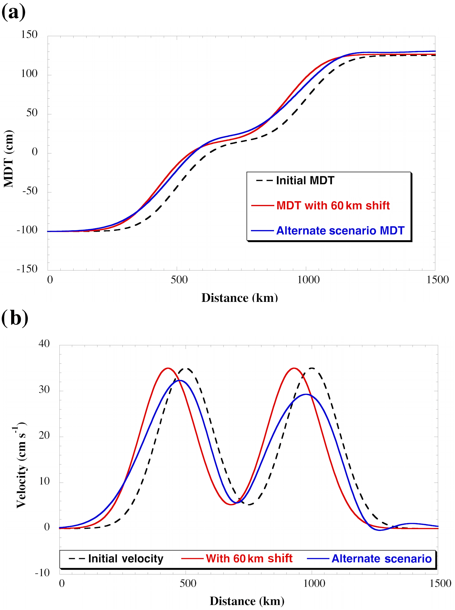
Figure 1(a) Mean dynamic topography in the Southern Ocean along a north–south meridian for three scenarios and (b) the corresponding geostrophic velocity, with positive values indicating eastward flow. The scenarios are an initial state (dashed black line), a shift in the two fronts south by 60 km with no change in magnitude or shape of the currents (red line), and no shift in the mean of the current but a change in the magnitude and shape (blue line).
Researchers using other methods also find little or no southern migration of the fronts or jets in the Southern Ocean as a whole. Graham et al. (2012) used a high-resolution model to show that the polar front and Subantarctic Front are constrained by bathymetry, even in increasing and shifting winds. Shao et al. (2015) utilized the skewness of sea level anomalies to identify front positions and found no southward motion but did find changes in the east Pacific correlated with the Southern Annular Mode. Chapman (2017a), using positions of fronts determined from the probability of jet locations, also found no significant southward movement but high interannual variability. Finally, Freeman and Lovenduski (2016a) used weekly estimates of the polar front position determined from satellite sea surface temperature (SST) gradients to show no significant southward shift between 2002 and 2014 on average, except in the Indian Ocean. They also found a statistically significant northward shift in the PF in part of the South Pacific.
Thus, recent studies all agree that the Subantarctic Front and polar front have not shifted south, even though there is evidence the winds have shifted south in the austral summer months (Swart and Fyfe, 2012). It should be noted that when averaged over the full calendar year, however, there has been no significant shift in the wind position (Swart and Fyfe, 2012).
In this paper, we develop a new method to study linear shifts in the position of the fronts in the Southern Ocean, based on tracking the location of envelopes of kinetic energy measured by satellite altimetry. It is known from modeling studies that the front positions are associated with increased kinetic energy, due to instabilities in the jets and interactions with bathymetry (Thompson et al., 2010; Thompson and Richards, 2011). After demonstrating that kinetic energy computed from along-track satellite altimetry forms relatively wide envelopes of enhanced energy that occur within the probability range of jets and fronts (e.g., Chapman, 2017a), we track the positions of these envelopes from 1993 until 2016 to quantify if the envelopes have shifted south by a statistically significant amount. Since kinetic energy is highest around fronts in the Southern Ocean (e.g., Thompson et al., 2010; Thompson and Richards, 2011; Chapman, 2017a), it follows that if the fronts have shifted south, then the envelope of high kinetic energy should also move by a comparable amount. We do not purport that our method derives the actual position of either a front or a jet due to the relatively wide swath of enhanced kinetic energy on either side of fronts related to variability in jets. Instead, we only purport that it can indicate shifts in the frontal position because if a front has shifted south by 100 km (for instance), then the band of enhanced kinetic energy should also shift south by a comparable amount. It is difficult to reconcile a frontal shift without a displacement of kinetic energy.
Since the kinetic energy calculation is based on estimating gradients of sea level anomalies, this approach is similar to other gradient methods for detecting fronts or jets (e.g., Chapman, 2014, 2017a; Gille, 2014; Freeman and Lovenduski, 2016a). It differs from these approaches, however, in that instead of determining individual gradients and tracking these over time, it looks for regions of high gradients (i.e., high energy) surround by regions of low gradient (i.e., low energy). This allows us to detect envelopes for every time period considered instead of only for a fraction of the time, allowing for better tracking of the change over time.
Section 2 will describe the data and methods used, while Sect. 3 will present results, including an evaluation of the method for detecting mean positions of fronts and for tracking their change over time. Section 4 will discuss the results in the context of previous studies and evaluate the usefulness of the method.
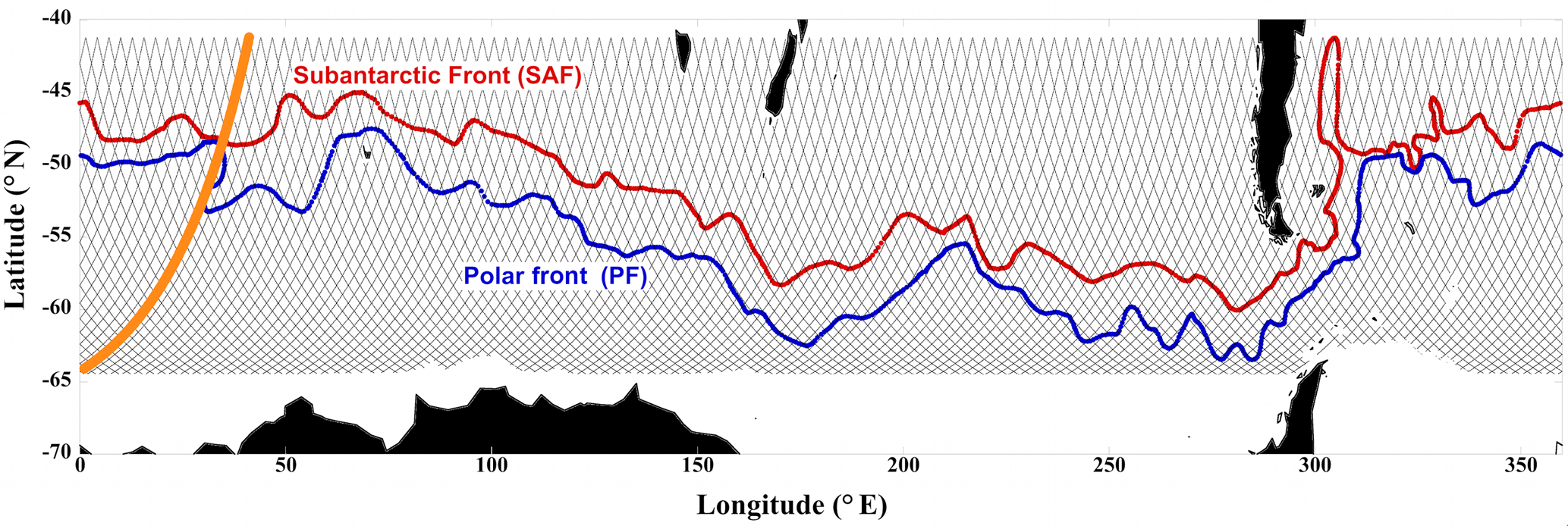
Figure 2Positions of the T/P, Jason-1, Jason-2, and Jason-3 ground tracks used for this study (black lines) and the approximate locations of the Subantarctic Front (red line) and the polar front (blue line) as estimated by Orsi et al. (1995). The orange track shows the location of the pass used in analysis shown in Figs. 3 and 4.
We utilize geostrophic surface current anomalies computed from the 24-year record of 1 Hz sea surface height (SSH) data along the TOPagraphy EXperiment/Poseidon (TOPEX/Poseidon, T/P) ground track in the Southern Ocean (Fig. 2). The altimetry data used are from four separate altimeter missions: TOPEX/Poseidon (January 1993–January 2002), Jason-1 (February 2002–July 2008), Jason-2 (August 2008–August 2016), and Jason-3 (August 2016–December 2016). Because the official TOPEX/Poseidon (T/P) geophysical data records (GDRs) have not been updated since the late 1990s, we utilize the corrected data products from the Integrated Multi-Mission Ocean Altimeter Data for Climate Research provided by Beckley et al. (2010) at the NASA Physical Oceanography Distributed Active Archive Center (PO.DAAC) site (https://podaac.jpl.nasa.gov/Integrated_Multi-Mission_Ocean_AltimeterData). Jason-1 data are from the GDR-C version and were downloaded from the NASA PO.DAAC site in June 2010. Jason-2 date are from the GDR-D version and were downloaded from NOAA National Oceanographic Data Center (NODC; ftp://ftp.nodc.noaa.gov/pub/data.nodc/jason2) between August 2012 and June 2016. Jason-3 data are also from the GDR-D version and were downloaded from NOAA NODC (ftp://ftp.nodc.noaa.gov/pub/data.nodc/jason3) on 7 and 8 August 2017.
We utilize the 1 Hz along-track SSH data from the four altimeters and compute sea surface height anomalies (SSHAs) by interpolating the DTU10 mean sea surface model (Andersen and Knudsen, 2009; http://www.space.dtu.dk/english/Research/Scientific_data_and_models/downloaddata) to the SSH location using bilinear interpolation. The DTU10 mean sea surface model is based on SSH from multiple altimeters averaged over 17 years in a rigorous and consistent manner (Andersen and Knudsen, 2009). T/P, Jason-1, and Jason-2 data were all included. All recommended geophysical and surface corrections (e.g., water vapor, ionosphere, sea state bias, ocean tides, inverted barometer) have been applied, to correct for biases introduced by atmospheric signal refraction and sea state effects (e.g., Chelton et al., 2001).
We utilize this record rather than the gridded products based on mapping SSH from multiple altimeters (e.g., Ducet et al., 2000; Pujol et al., 2016) because the along-track data have a finer resolution in space (6.9 km along the ground track) and we recently demonstrated that the mapped altimetry data underestimated eddy kinetic energy (EKE) throughout the Southern Ocean by as much as 60–70 % compared to along-track data (Hogg et al., 2015). While the along-track sea level anomalies are filtered to reduce noise and thus may attenuate some signal, the filtering used (described later in this section) is less than that used for the mapped data, which uses observations from as long as 20 days and 200 km away to influence the mapped value. By filtering only along-track data, the time differences are small (a few minutes at most), and the spatial influence is less than 100 km. Tests with unfiltered data accounting for estimated random noise in the sea level anomaly data suggests that attenuation of kinetic energy is minimal with this approach and, more importantly, that the shape of the kinetic energy envelope does not significantly change.
One can only compute EKE from along-track data at crossover points, where the ascending and descending ground tracks cross (Fig. 2). Knowing the ground track angle with the north meridian (θ), one can compute the zonal (dη∕dy) and meridional gradients (dη∕dx) of SSHA directly from the gradients of SSHA for the ascending pass (dη∕drasc) and descending pass (dη∕drdes) using simple geometry (Parke et al., 1987):
noting that this formulation assumes that the gradients represent the derivative of the northern SSHA relative to the southern SSHA (for both the ascending and descending passes). Once this is computed, the velocities can be computed directly from the zonal and meridional gradients:
where g is the acceleration due to gravity and f is the Coriolis parameter.
This formulation assumes that the velocity field has not changed significantly between the times the two passes fly over the crossover point. At high latitudes, the majority of crossovers (> 78 %) have a time separation of less than 3 days. At 40∘ S, the average propagation speed of an eddy is about 3 cm s−1 (Chelton et al., 2007), meaning the eddy would have only been displaced by 8 km at most over this period. At higher latitudes, this is even less. Considering that the diameter of eddies at these latitudes is of the order of 100 km (Chelton et al., 2007), the movement is not large enough to cause a significant change in velocity at the point. The primary problem with velocities computed from crossovers is the smaller number compared to using gridded data or the time-varying, anomalous geostrophic current normal to the ground track (uT). This can be computed directly from the derivative of the SSH anomaly (η) along the ground-track distance (dr) from
This cross-track current is a projection of both the zonal (u) and meridional (v) components of the full anomalous velocity field. However, neither u nor v can be determined unambiguously from uT. Here, we merely examine the variability in uT without making any assumptions concerning how it may be related to the full velocity or to u and v.
Because derivatives of SSHA (Eqs. 1 and 3) have to be computed numerically (here, center differences are used) and η contains significant noise at the 1 Hz sampling rate of the altimeters, we optimally interpolate η along-track using a model of the covariance of the signal and error. We used the method of Wunsch (1996, Chap. 3) and a covariance function modeled as a Gaussian with a roll-off of 98 km and random noise of 2 cm, which was determined from the autocovariance of all TOPEX/Poseidon, Jason-1, and Jason-2 SSHA data from 1993 to 2015 between 40 and 65∘ S.
Once uT(t) was computed at each 1 s bin along the ground tracks in Fig. 2 for each 10-day repeat cycle, the cross-track kinetic energy (CKE) was computed as CKE( 0.5 uT(x,t)2, where x here is used to denote a generic 1 s bin along the ground track. We also computed the full EKE at the more limited crossover points as EKE( 0.5(.
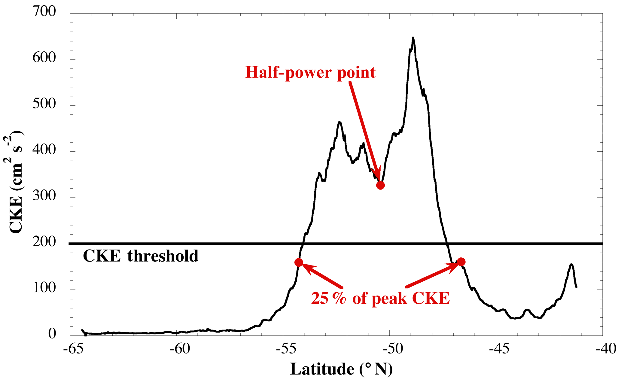
Figure 3An example profile of mean CKE (1993–2016) along a ground track in the southern Indian Ocean (shown in orange in Fig. 2), demonstrating the location of the half-power point and the locations of the southern and northern boundaries of the enhanced CKE envelope. See text for details of the computations.
The CKE values were averaged over the entire 24-year record and examined for each ground track segment (both ascending and descending) to judge where CKE was exceptionally high (Fig. 3). We also computed CKE using the raw values of SSHA and compared to that computed with optimal interpolation. The locations of high CKE were the same, although values were significantly higher with the unsmoothed data. The quiescent regions of the ocean also showed considerably more noise, making it more difficult to determine boundaries of elevated CKE. For this reason, the values determined from the optimally interpolated data were used.
Several criteria were utilized to quantify where the high CKE values were considered to be associated with fronts. First, we constrained the southern boundary to be 5∘ south of the Orsi et al. (1995) values of the PF and the northern boundary to be 5∘ north of the SAF. Secondly, we used a lower limit for CKE of 200 cm2 s−2 for detection and tested that the width of the envelope of high CKE above the lower limit was at least 100 km. The requirement that the envelope be greater than 100 km was done to reduce the impact of eddies in an otherwise quiescent region, since the diameter of eddies in the Southern Ocean is about 100 km. The CKE lower limit was determined via iteration with different limits. For each case, the average center of the CKE envelope averaged over 24 years (based on the mean of the first and last points to exceed the lower limit) was computed and compared visually to the Orsi et al. (1995) front positions. 200 cm2 s−2 was selected because there were a significant amount of CKE envelope centers clustered around the Orsi et al. (1995) fronts and the envelopes were found for every 10-day repeat cycle. Using a higher limit resulted in fewer detections, especially when smaller time averages were used. Using a lower limit, we could find more potential front positions based on CKE, but many were far from the front positions estimated by Orsi et al. (1995) and other authors (e.g., Kim and Orsi, 2014; Freeman and Lovenduski, 2016a; Chapman, 2017a).
An example of a detected high CKE envelope is shown in Fig. 3, based on the average of CKE between 1993 and 2015 computed from T/P-Jason satellite pass 207 in the south Indian Ocean. This pass starts at 64.3∘ S near the prime meridian and extends to 41.2∘ S and 41∘ E longitude. There is clearly a wide envelope of enhanced CKE greater than 200 cm2 s−2 between 55 and 47∘ S.
The mean CKE profile pictured in Fig. 3 has multiple local maxima, most likely associated with variability in the narrow jets that surround the front. They may also represent two separate fronts (and frontal-related jets) that are close in space. Some frontal climatologies find that the SAF and PF are separated by fewer than 100 km in the south Indian Ocean (between 30 and 40∘ E), the South Pacific (between 220 and 230∘ E), and the South Atlantic (310 and 330∘ E; Fig. 2). CKE computed in these areas may encompass energy around both fronts. However, if the fronts have both shifted south (as reported in some studies), then CKE should also shift south and so tracking CKE should observe the shifts in frontal location.
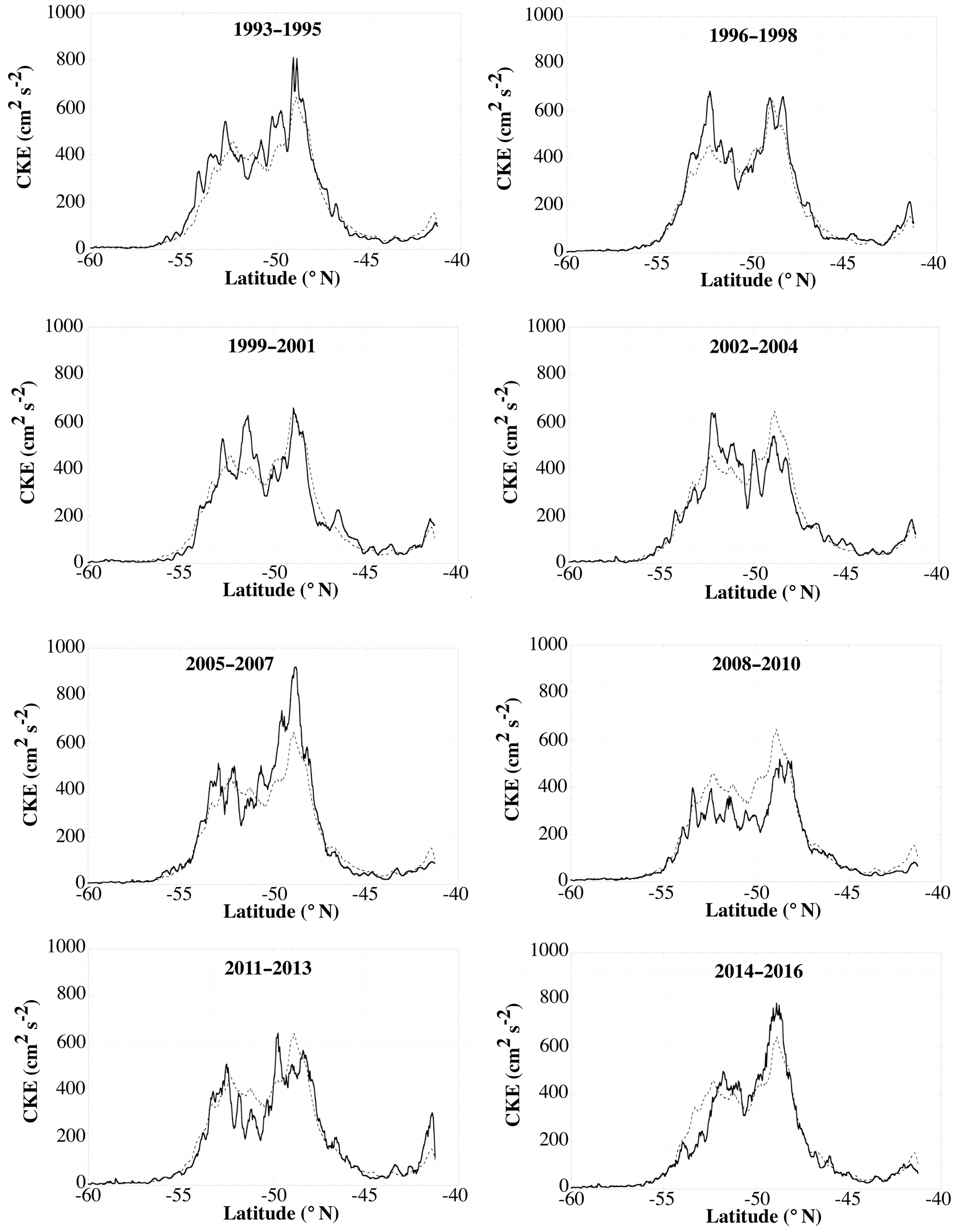
Figure 4Three-year averages of CKE estimated along pass shown in Fig. 2 (solid lines) along with the long-term mean from 1993 to 2016 (dotted line).
Figure 4 shows the behavior of CKE along this pass for different 3-year periods. Note that the number of clearly defined maxima ranges from a low of four for the 2014–2016 average to nine in 1993–1995. Note that even with a fixed and stationary front, there may be highly variable locations of peaks in CKE around the front, due to the meandering and disappearance/formation of jets (e.g., Chapman, 2017a). Thus, tracking the specific jet locations is not an optimal method of tracking frontal shifts. While other studies have estimated positions of these maxima in SSHA gradients at daily intervals (e.g., Chapman, 2017a), one does not obtain a consistent number of maxima each time, making the determination of shifts difficult. Moreover, note that although there are two general peaks in CKE in the long-term mean profile, the minimum between them is still higher than 200 cm2 s−2. A minimum is also not well defined in several of the shorter averaging periods (for example, 2008–2010).
Thus, instead of attempting to track all the maxima of CKE individually – analogous to tracking the steepest gradients, as in Thompson et al. (2010), Graham et al. (2012), and Chapman (2017a) – we track an estimate of the center of the envelope of enhanced CKE, as it exists in all averaging periods. The assumption we make in doing this is that the localized maxima are associated with variable jets but the position of the envelope of high CKE is related to the general position of the front and that if the front has systematically shifted then the CKE envelope will have shifted as well. Other studies have tracked the mean latitude of the integrated transport computed between dynamic height contours that are picked to represent the southern boundary and the northern boundary that encompass all the fronts in the ACC (Gille, 2014). One issue with this approach is how to uniquely determine the northern and southern boundary contours without potentially biasing the result (e.g., using a priori fixed boundaries and ignoring that they might have shifted). The method we propose will determine the boundaries of the integration uniquely for each pass based solely on the level of CKE relative to the peak of the enhanced CKE envelope. Moreover, it allows for two or more distinct CKE envelopes along each pass (i.e., related to different fronts), whereas the Gille (2014) method can only compute one mean latitude for all fronts in between the prescribed southern and northern boundaries. Thus, our method is more flexible in determining boundaries around any particular front, provided the orientation of the ground track is such that the majority of jets are perpendicular to it.
There are many different ways to compute a “center” of the envelope, ranging from the average of the two end points to a centroid calculation to computing the point where the integral of CKE over distance is balanced on both sides, which we call the “half-power point.” We have selected the latter to use, as it defines a center closer to the peak of CKE in the envelope. This is advantageous when the CKE curve is slightly skewed, with less magnitude on one side and more on the other. Assuming that the variability (and hence CKE) would be highest near the front (i.e., what is assumed in studies using the gradient method), finding a center of the envelope that is biased toward peak CKE is a reasonable approach.
The half-power point (xmid) is computed so that
where xsouth and xnorth are computed by first finding the maximum of CKE in the envelope above 200 cm2 s−2 and then finding the first value to the north just below 25 % of that peak along with the similar value to the south (shown in Fig. 3). Values other than 25 % of the peak were tested. Using values greater than this, up to 50 %, resulted in no significant difference in the half-power point. Using values smaller resulted in some boundaries not being defined. Thus, 25 % of peak CKE was considered reasonable. If multiple regions of enhanced CKE were found along the same track, this process was carried out for each of them. This was done for all the 24-year mean CKE profiles to establish the mean locations of the fronts between 1993 and 2016.
A similar procedure was done for CKE averaged over discrete 3-year intervals, starting in January 1993 and ending in December 2016. A 3-year average was used to reduce the influence of individual eddies on determining the envelope and to reduce interannual variations in the front position, which have been observed in other studies at some locations (e.g., Kim and Orsi, 2014; Shao et al., 2015). In particular, Kim and Orsi (2014) and Shao et al. (2015) found significant correlation with the Southern Annular Mode, which has a quasi-biennial oscillation (Hibbert et al., 2010). By averaging over 3 years, we found eight distinct, statistically uncorrelated samples of CKE for each ground track from which to deduce shifts in the half-power point. We tested different averaging periods (ranging from 1 to 4 years) but found that the estimate in overall shift in the half-power point over the 24-year period was insensitive to the choice.
The first thing tested was how well CKE represented the full EKE. If CKE does not have the same general shape as EKE, then using it as a proxy for EKE to determine high-energy envelopes is not valid. After finding satellite passes with high CKE as discussed in Sect. 2, EKE was computed along the same pass, using the crossover method (Eqs. 1 and 2).
Although CKE is lower than EKE along all ground tracks (see Fig. 5 for examples), the pattern of KE (kinetic energy) rise and then fall is virtually identical. CKE, however, has the benefit of higher and more regular sampling. Thus, we conclude that CKE is a reasonable proxy for locating front positions even though it may not be useful for quantifying the full energy of the anomalous currents.
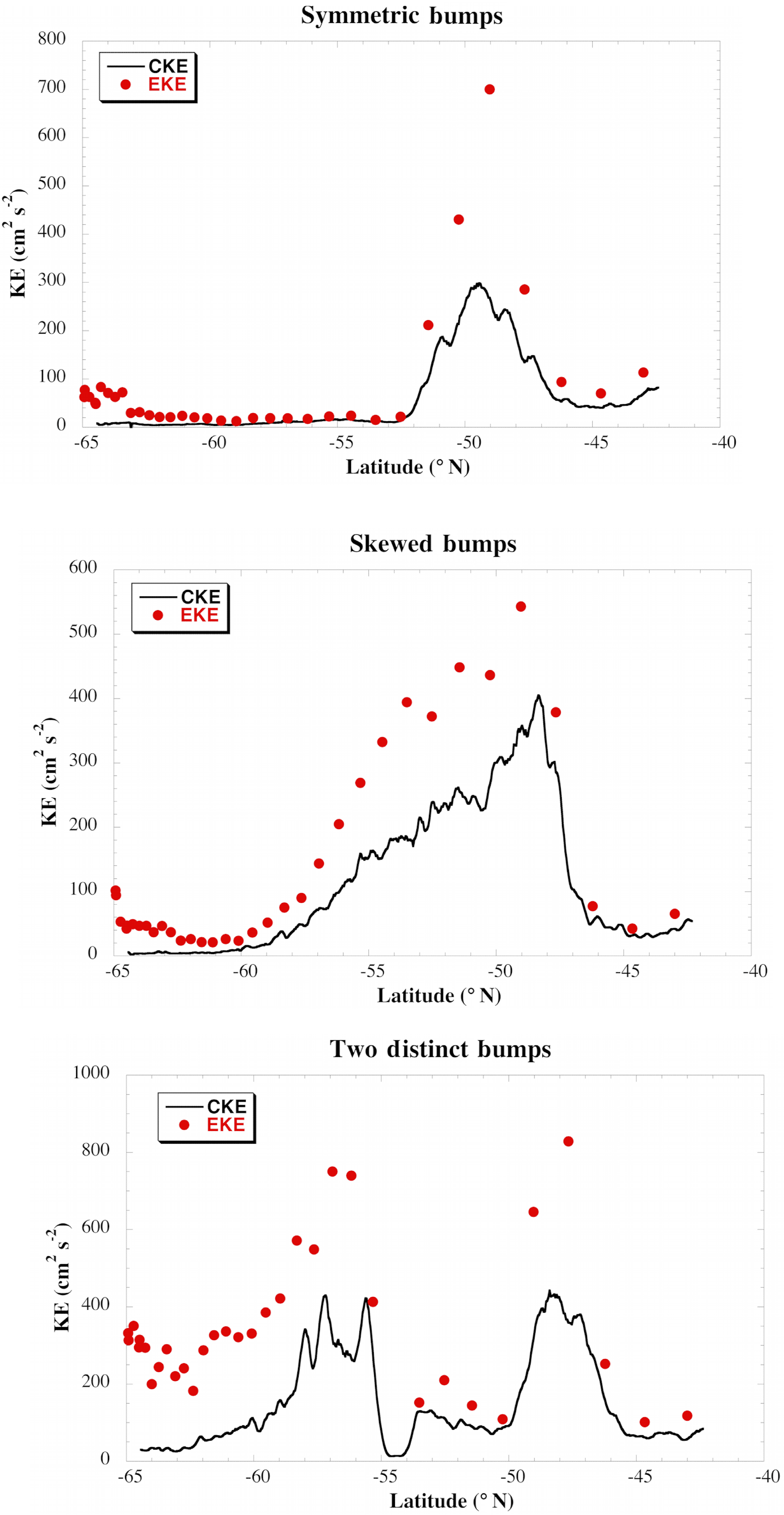
Figure 5Examples of the three types of CKE profiles found (black lines), along with the value of the full EKE computed at crossover points.
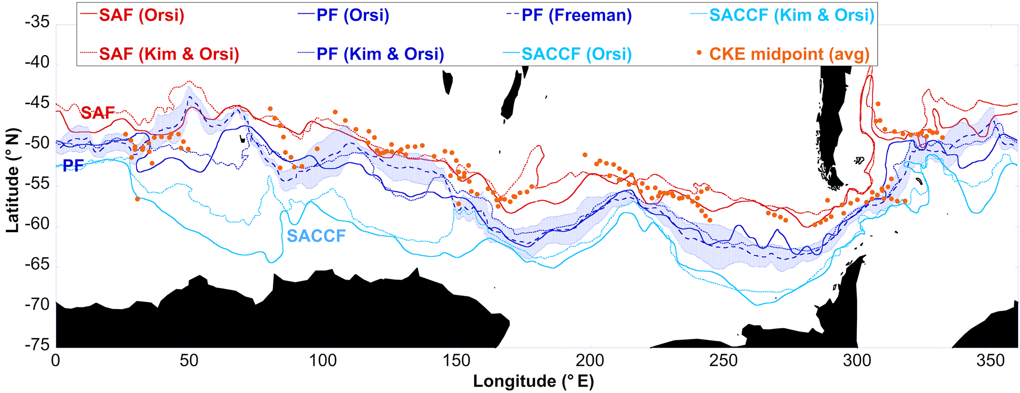
Figure 6Mean positions of fronts estimated from CKE (orange dots) along with estimates from other authors: Orsi et al. (1995), computed using hydrographic sections; Kim and Orsi (2014), based on contours of dynamic topography; and Freeman and Lovenduski (2016a), based on gradients of sea surface temperature. The Orsi et al. (1995) fronts were downloaded from https://gcmd.nasa.gov/records/AADC_southern_ocean_fronts.html. The Freeman and Lovenduski fronts were downloaded from https://doi.pangaea.de/10.1594/PANGAEA.855640 (Freeman and Lovenduski, 2016b). The Kim and Orsi (2014) fronts were provided by Yong Sun Kim upon request.
Four general types of enhanced CKE were found (Figs. 4 and 5). In most regions, the envelope in CKE is more or less symmetrical (52 % of cases). Only a few profiles have two distinct regions of enhanced CKE that were identified, with a clearly defined minimum below 200 cm2 s−2 between them in all time periods (3 % of cases). Overall, 20 % of the passes have multiple peaks that vary in time but have no consistent minimum between the peaks (i e., Fig. 4), while 25 % have a skewed envelope (Fig. 5), with a long rise in CKE followed by a sharp drop-off. In all cases, though, the shape of the CKE envelope closely follows that of EKE, although the amplitude was attenuated, by anywhere from 25 to 50 %. Having closer samples of CKE, however, allows for a better computation of the half-power point and possible shifts.
Figure 6 shows the locations of the half-power points determined from the mean CKE profiles, along with an estimate of the front position based on different methods: density gradients from historical hydrographic sections (Orsi et al., 1995), dynamic topography contours (Kim and Orsi, 2014), and the gradient of sea surface temperature (Freeman and Lovenduski, 2016a). There are two estimates of the SAF and Southern ACC front (SACCF) and three of the PF. One of the PF estimates (from Freeman and Lovenduski, 2016a) includes the standard deviation of the daily estimates.
It is important to note the large differences in estimates for the same front, which indicates how difficult it is to determine fronts in a highly variable current system like the ACC. For instance, in the Indian Ocean at 50∘ E, Freeman and Lovenduski (2016a) find the PF at the same location that Orsi et al. (1995) found the SAF, while Kim and Orsi (2014) find it significantly farther south. The SAF determination using the contour method (Kim and Orsi, 2014) is substantially farther north than the one determined from hydrographic data (Orsi et al., 1995) at most longitudes. These differences are likely due to differences in the time span, differences in methodologies, and uncertainty in the data utilized. All lead to a level of uncertainty in the determination of a specific front at any time.
The half-power points of enhanced CKE generally occur near or between the fronts estimated by different methods (i.e., the three different PF estimates), indicating that they are at least within the uncertainty bounds of frontal detection by other methods. Some values are at locations either north or south of the other front estimates by as much as 3∘, but it should be noted that the standard deviation of the PF estimated by Freeman and Lovenduski (2016a, b) averages 2–3∘. Using a PF variability statistic as an indicator of the variability of all fronts, one can conclude that the location of CKE half-power points is well within the level of expected frontal variability and so not statistically too distant from a front location.
One may question whether the relatively wide envelopes of enhanced CKE overlap more than one front. This is a possibility, but if both fronts have moved south as some have argued (e.g., Sokolov and Rintoul, 2009b), then the CKE envelope should also shift, regardless of whether it includes one or two fronts. If the exact frontal location was known at any time, one could judge how well the CKE envelope (or half-center) point was associated with just one front. But considering the disagreement in climatologies (e.g., Fig. 5) and the intrinsic variability in the front, this is impossible to test. One can, however, compute the distance from the CKE half-power point to the southern boundary (for those points that are nearest a climatological SAF position) and the distance with the northern boundary (for those that are nearest the PF) and compare this to the distance between the climatological positions of these fronts. Note that the distances must be computed along the ground tracks and not simply taken as the meridional distance at the longitude of the CKE half-power point.
The average distance between the half-power point and either northern or southern boundary is 541 km with a standard deviation of 196 km. The average distance between the Kim and Orsi (2014) PF and SAF along the ground track passes is 706 km with a standard deviation of 407 km. We used the Kim and Orsi (2014) front positions as these data were on a regular grid, which made interpolation to the ground track positions easier and was computed over the roughly the same time span as the CKE estimates. From these statistics, we conclude that the CKE envelopes should generally only encompass either the PF or the SAF, although even if they did not, it should not preclude one from using statistics of the CKE half-power point to deduce shifts in the fronts, provided they are both shifting, as has been theorized.
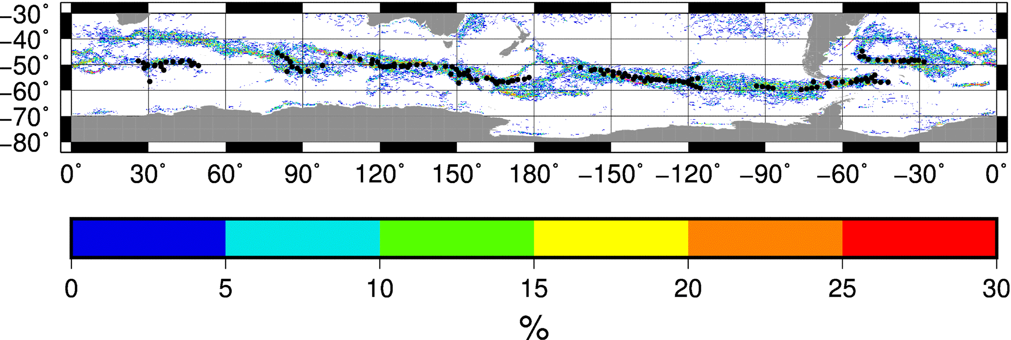
Figure 7Mean positions of fronts estimated from CKE (black dots) along with the percent occurrence of a jet between 1993 and 2014 computed by Chapman (2017a). Data were downloaded from https://doi.org/10.5061/dryad.q9k8r (Chapman, 2017b). The percent occurrence of the jet was computed by calculating the number of times a jet occurred in the daily files, dividing by the total number of days between January 1993 and December 2014 and multiplying by 100.
Another method for determining frontal position is to examine the probability of jets occurring (Chapman, 2017a; Fig. 7). The CKE-defined mean front positions lie within the probability envelopes, giving more confidence that the CKE measure is providing a comparable measure of frontal position in many areas. The only location where CKE-defined fronts do not agree well with the probability field from Chapman (2017a) is just west of the dateline, where two points lie between levels of high jet (and hence front) probability. However, it should be noted that Chapman finds jets in the two areas north and south of the CKE half-power points less than 10 % of the time and that the northern cluster lies on the northern edge of the enhanced CKE envelope. Although the half-power points are slightly south of this along these two passes, this is due to high CKE (in excess of 200 cm2 s−2) down to 58∘ S, where Chapman (2017a) detects few jets. It is unclear why Chapman (2017a) detects few jets in this region of high CKE, but it should be noted that this represents only 1 % of the samples compared.
The comparison between CKE half-power points and front climatologies provides reassurance that the method developed in Sect. 2 is successfully detecting regions of high energy related to jets around fronts. Since the movement of jet positions has been used to estimate the movement of the fronts (e.g., Chapman, 2017a), a comparable calculation with positions of high CKE seems reasonable. The majority of the estimated half-power points follows the SAF and is most likely due to the front (and jets) moving perpendicular to the ground tracks. This method will tend to only detect high CKE when the front is moving from northwest to southeast for an ascending pass and from southwest to northeast for a descending pass. This method also only works in regions where the front is associated with highly variable jets, which does not occur at every longitude along the front (e.g., Chapman, 2017a).
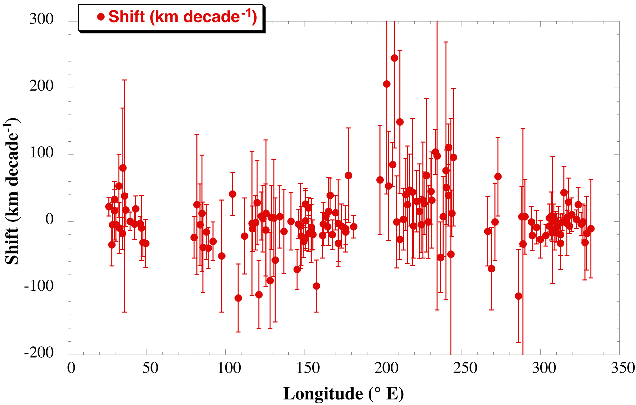
Figure 8Estimated trend in the half-power point of CKE for each location shown in Figs. 6 and 7, as a function of latitude. Error bars represent the 90 % confidence interval.
To quantify the movement of the envelope of enhanced CKE, a linear trend is fit to the eight estimations of the half-power point from 1993 to 2016 for each location shown in Figs. 5 and 6. An analysis of the residuals about the trend indicated that they were random (lag-1 autocorrelation < 0.1 for all cases), so standard error was computed by scaling the formal error from the covariance matrix determined in ordinary least squares by the standard deviation of the residuals. This was also scaled up to account for the degrees of freedom lost by estimating the trend by sqrt(n∕nEDOF), where n= 8 and nEDOF= 6. Finally, the 90 % confidence interval was computed by scaling by 1.94 for 6 effective degrees of freedom assuming a normal t distribution of the residuals.
The results indicate considerable regional variability in the change in the half-power point over 24 years, with large uncertainty bars (Fig. 8). This is due to the substantial temporal variability in the positions, which can be seen in Fig. 4, where the leading edge of the CKE envelope varies by over 1 degree of latitude (over 100 km) between 1993–1995 and 2011–2012. To better see significant changes outside the uncertainty (90 % confidence) interval, one can compute the signal-to-noise ratio (SNR = trend/uncertainty). Examining this (Fig. 9), one can see that there are some regions where the half-power point has moved southward by a significant distance over the last 24 years (13.6 % of points), but there are also points where it has moved north (9.6 %). For the majority of points (76.8 %), there is no statistically significant change, meaning no movement of the front is as likely as either a southward or northward shift due to the high variability in 3-year positions.
The results from the analysis of the positions of enhanced kinetic energy suggest no overall shift in the frontal positions across the Southern Ocean but some large, localized movements. The region indicative of some southward shift between 90 and 170∘ E is in approximately the same area where Kim and Orsi (2014) and Freeman and Lovenduski (2016a) also reported large shifts between 1992 and 2011 and 2002 and 2014, respectively. However Freeman and Lovenduski only examined the polar front, and Kim and Orsi (2014) only found large shifts in the PF and the southern ACC front. They found shifts of the of order 50–100 km in the SAF where the points in this study cluster, which is considerably smaller than the individual shifts we find between 90 and 170∘ E along the SAF. However, the overall average over the region between 90 and 170∘ E (−29 km per decade, or −66.7 km in 23 years), is consistent with what Kim and Orsi (2014) found.
Kim and Orsi (2014) and Freeman and Lovenduski (2016a) also found slight northward shifts in the front positions in the southeast Pacific between 200 and 270∘ E. We find that some locations in this region, where the CKE half-power points cluster around the SAF, also have a significant northward shift. Kim and Orsi (2014) found that the shift in the SAF was about 30–40 km between 1992 and 2011. Our results suggest larger shifts in some areas; averaged over the area, our results are 46 km per decade to the north, or 106 km from 1993 to 2015, which is consistent with the average over the region computed by Freeman and Lovenduski (2016a) from sea surface temperature data but for the polar front.
Kim and Orsi (2014) suggest that the shift in the fronts in the Indian Ocean were not directly related to shifts in winds but instead were caused by an expansion of the Indian subtropical gyre. They linked the shift in the southeastern Pacific to wind changes related to mainly the Southern Annular Mode in that region (Kim and Orsi, 2014).
Overall, this study supports the recent studies by Kim and Orsi (2014), Gille (2014), Freeman and Lovenduski (2016a), and Chapman (2017a). All find that, while the frontal positions of the ACC are highly variable in time, there is no statistically significant shift in the fronts to the south on average. This study utilized a novel technique to reach this conclusion, which adds to the robustness of evidence that there has not been a shift in the frontal positions. Thus, while the fronts may eventually shift south in a warming climate, there is no strong evidence that it is happening at the moment.
Other studies have shown significant positive trends in the Southern Ocean that have been connected to the warming climate. These include changes in the ocean heat content in the upper ocean between the 1930s–1950s and the 1990s (e.g., Böning et al., 2008; Gille, 2008), increases in the heat content of deep water between the 1990s and 2005 (e.g., Purkey and Johnson, 2010), and increases in eddy kinetic energy in the Indian and Pacific oceans since 1993 (Hogg et al., 2015). Observational evidence of shifts in the winds, however, indicates that while there may be a slight southward shift in winds during the Southern Hemisphere summer, the overall yearly average shift is not significant (Swart and Fyfe, 2012). Thus, the growing consensus that fronts have not shifted to the south, on average, is consistent with observations of no significant shift in the yearly averaged winds.
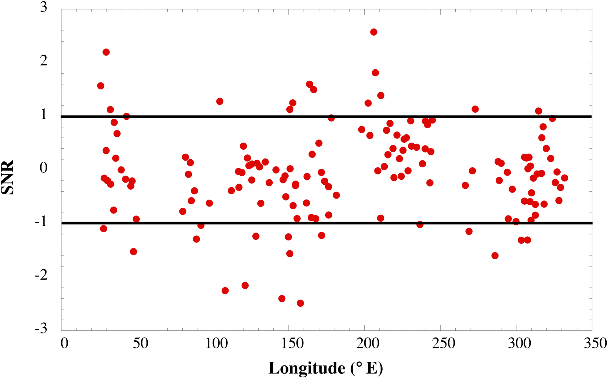
Figure 9SNR (trend/error in Fig. 8). Values larger than 1 indicate a statistically significant northern shift. Values smaller than −1 indicate a statistically significant southern shift. Values between ±1 indicate no statistically significant shift.
The only evidence supporting a hypothesis that ACC fronts have shifted southward since the 1990s comes from mapping the location of contours of constant dynamic topography over time (e.g., Sokolov and Rintoul, 2009b; Kim and Orsi, 2014). As Gille (2014) argued and as we have demonstrated based on a simple thought experiment (Fig. 1), there are other equally plausible explanations for the apparent southern shift in the contours. Considering that four different techniques – location of mean transport (Gille, 2014), maximum SST gradients (Freeman and Lovenduski, 2016a), probability of jet positions (Chapman, 2017a), and the location of enhanced kinetic energy (this study) – all agree that the fronts have not moved significantly on average, one has to conclude that the method of using dynamic topography contours to detect changes in front position is too sensitive to sea level rise to be useful for determining shifts in frontal positions, although it may prove useful for determining the mean position, as Chapman (2017a) has argued.
TOPEX/Poseidon data come from the Integrated Multi-Mission Ocean Altimeter Data for Climate Research provided by Beckley et al. (2010) at the NASA Physical Oceanography Distributed Active Archive Center (PO.DAAC) site (https://podaac.jpl.nasa.gov/Integrated_Multi-Mission_Ocean_AltimeterData). Jason-1 data are from NASA PO.DAAC ( https://podaac.jpl.nasa.gov/dataset/JASON-1_L2_OST_GPN_E). Jason-2 data are from the NOAA National Oceanographic Data Center (NODC; ftp://ftp.nodc.noaa.gov/pub/data.nodc/jason2). Jason-3 data are from NOAA NODC (ftp://ftp.nodc.noaa.gov/pub/data.nodc/jason3). The DTU10 mean sea surface model is from Andersen and Knudsen (2009) and can be downloaded from http://www.space.dtu.dk/english/Research/Scientific_data_and_models/downloaddata. Locations of the PF are from Freeman and Lovenduski (2016b) and can be downloaded from https://doi.org/10.1594/PANGAEA.855640.
The author declares that he has no conflict of interest.
The author would like to thank Christopher Chapman and an anonymous reviewer
for their extensive comments on an earlier draft of this paper. Their many
suggestions helped the author improve the paper substantially. This research
was carried out under grant number NNX13AG98G from NASA and a grant from
NOAA for the NASA/NOAA Ocean Surface Topography Science Team.
Edited by: Matthew Hecht
Reviewed by: Christopher Chapman and one anonymous referee
Andersen, O. B. and Knudsen, P.: DNSC08 mean sea surface and mean dynamic topography models, J. Geophys. Res., 114, C11001, https://doi.org/10.1029/2008JC005179, 2009.
Beckley, B. D., Zelensky, N. P., Holmes, S. A., Lemoine, F. G., Ray, R. D., Mitchum, G. T., Desai, S., and Brown, S. T.: Assessment of the Jason-2 Extension to the TOPEX/Poseidon, Jason-1 Sea-Surface Height Time Series for Global Mean Sea Level Monitoring, Mar. Geod., 33, 447–471, https://doi.org/10.1080/01490419.2010.491029, 2010
Belkin, I. M. and Gordon, A. L.: Southern Ocean fronts from the Greenwich meridian to Tasmania, J. Geophys. Res., 101, 3675–3696, 1996.
Böning, C. W., Dispert, A., Visbeck, M., Rintoul, S. R., and Schwarzkopf, F. U.: The response of the Antarctic circumpolar current to recent climate change, Nat. Geosci., 1, 864–869, 2008.
Chapman, C. C.: Southern Ocean jets and how to find them: Improving and comparing common jet detection methods, J. Geophys. Res.-Oceans, 119, 4318–4339, https://doi.org/10.1002/2014JC009810, 2014.
Chapman, C. C.: New perspectives on frontal variability in the Southern Ocean, J. Phys. Oceanogr., 47, 1151–1168, https://doi.org/10.1175/JPO-D-16-0222.1, 2017a.
Chapman, C. C.: Data from: New perspectives on frontal variability in the southern ocean, Dryad Digital Repository, https://doi.org/10.5061/dryad.q9k8r, 2017b.
Chelton, D. B., Ries, J. C., Haines, B. J., Fu, L.-L., and Callahan, P. S.: Satellite altimetry, in: Satellite Altimetry and Earth Science, International Geophysics Series, edited by: Fu, L.-L. and Cazanave, A., Vol. 69, Academic Press, San Diego, CA, 1–131, 2001.
Chelton, D. B., Schlax, M. G., Samelson, R. M., and de Szoeke, R. A.: Global observations of large oceanic eddies, Geophys. Res. Lett., 34, L15606, https://doi.org/10.1029/2007GL030812, 2007.
Cunningham, S. A., Alderson, S. G., King, B. A., and Brandon, M. A.: Transport and variability of the Antarctic Circumpolar Current in Drake Passage, J. Geophys. Res., 108, 8084, https://doi.org/10.1029/2001JC001147, 2003.
Ducet, N., Le Traon, P.-Y., and Reverdin, G.: Global high resolution mapping of ocean circulation from TOPEX/Poseidon and ERS-1 and -2, J. Geophys. Res., 105, 19477–19498, 2000.
Fyfe, J. C. and Saenko, O. A.: Simulated changes in the extratropical Southern Hemisphere winds and currents, Geophys. Res. Lett., 33, L06701, https://doi.org/10.1029/2005GL025332, 2006.
Freeman, N. M. and Lovenduski, N. S.: Mapping the Antarctic Polar Front: weekly realizations from 2002 to 2014, Earth Syst. Sci. Data, 8, 191–198, https://doi.org/10.5194/essd-8-191-2016, 2016a.
Freeman, N. M. and Lovenduski, N. S.: Mapping the Antarctic polar front: weekly realizations from 2002 to 2014, links to NetCDF file and MPEG4 movie, PANGEA, https://doi.org/10.1594/PANGAEA.855640, 2016b.
Gille, S: Decadal-scale temperature trends in the Southern Hemisphere Ocean, J. Climate, 21, 4749–4765, 2008.
Gille, S. T.: Meridional displacement of the Antarctic Circumpolar Current, Philos. T. R. Soc. A, 372, 20130273, https://doi.org/10.1098/rsta.2013.0273, 2014.
Graham, R. M., De Boer, A. M., Heywood, K. J., Chapman, M. R., and Stevens, D. P.: Southern Ocean fronts: Controlled by wind or topography?, J. Geophys. Res.-Oceans, 117, C08018, https://doi.org/10.1029/2012JC007887, 2012.
Hibbert, A., Leach, H., Woodworth, P., Hughes, C., and Rousseno, V.: Quasi-biennial modulation of the Southern Ocean coherent mode, Q. J. R. Meteor. Soc., 136, 755–768, https://doi.org/10.1002/qj.581, 2010.
Hogg, A., Meredith, M. P., Chambers, D. P., Abrahamsen, E. P., Hughes, C. W., and Morrison, A. K.: Recent trends in the Southern Ocean eddy field, J. Geophys. Res.-Oceans, 120, 257–267, https://doi.org/10.1002/2014JC010470, 2015.
Kim, Y. S. and Orsi, A. H.: On the variability of Antarctic Circumpolar Current fronts inferred from 1992-2011 altimetry, J. Phys. Oceanogr., 44, 3054–3071, https://doi.org/10.1175/JPO-D-13-0217.1, 2014.
Langlais, C., Rintoul, S. R., and Schiller, A.: Variability and mesoscale activity of the Southern Ocean fronts: Identification of a circumpolar coordinate system, Ocean Modell., 39, 79–96, https://doi.org/10.1016/j.ocemod.2011.04.010, 2011.
Nowlin, W. D. and Clifford, M.: The kinematic and thermohaline zonation of the Antarctic Circumpolar current at Drake Passage, J. Mar. Res., 40, 481–507, 1995.
Orsi, A. H., Whitworth III, T., and Nowlin Jr., W. D.: On the meridional extent and fronts of the Antarctic Circumpolar Current, Deep-Sea Res. Pt. I, 42, 641–673, https://doi.org/10.1016/0967-0637(95)00021-W, 1995.
Parke, M. E., Stewart, R. H. , Farless, D. L., and Cartwright, D. E.: On the choice of orbits for an altimetric satellite to study ocean circulation and tides, J. Geophys. Res., 92, 11693–11707, 1987.
Pujol, M.-I., Faugère, Y., Taburet, G., Dupuy, S., Pelloquin, C., Ablain, M., and Picot, N.: DUACS DT2014: the new multi-mission altimeter data set reprocessed over 20 years, Ocean Sci., 12, 1067–1090, https://doi.org/10.5194/os-12-1067-2016, 2016.
Purkey, S. G. and Johnson, G. C.: Warming of global Abyssal and deep southern ocean waters between the 1990s and 2000s: Contributions to global heat and sea level rise budgets, J. Climate, 23, 6336–6351, https://doi.org/10.1175/2010JCLI3682.1, 2010.
Sallee, J. B., Speer, K., and Morrow, R.: Response of the Antarctic Circumpolar Current to atmospheric variability, J. Climate, 21, 3020–3039, https://doi.org/10.1175/2007JCLI1702.1, 2008.
Shao, A. E., Gille, S. T., Mecking, S., and Thompson, L.: Properties of the Subantarctic Front and Polar Front from the skewness of sea level anomaly, J. Geophys. Res.-Oceans, 120, 5179–5193, https://doi.org/10.1002/2015JC010723, 2015.
Sokolov, S. and Rintoul, S. R.: Multiple jets of the Antarctic Circumpolar Current south of Australia, J. Phys. Oceanogr., 37, 1394–1412, https://doi.org/10.1175/JPO3111.1, 2007.
Sokolov, S. and Rintoul, S. R.: Circumpolar structure and distribution of the Antarctic Circumpolar Current fronts: 1. Mean circumpolar paths, J. Geophys. Res., 114, C11018, https://doi.org/10.1029/2008JC005108, 2009a.
Sokolov, S. and Rintoul, S. R.: Circumpolar structure and distribution of the Antarctic Circumpolar Current fronts: 2. Variability and relationship to sea surface height, J. Geophys. Res., 14, C11019, https://doi.org/10.1029/2008JC005248, 2009b.
Swart, N. and Fyfe, J. C.: Observed and simulated changes in the Southern Hemisphere surface westerly wind-stress, Geophys. Res. Lett., 39, L16711, https://doi.org/10.1029/2012GL052810, 2012.
Thompson, A. F. and Richards, K. J.: Low frequency variability of Southern Ocean jets, J. Geophys. Res., 116, C09022, https://doi.org/10.1029/2010JC006749, 2011.
Thompson, A. F., Haynes, P. H., Wilson, C., and Richards, K. J.: Rapid Southern Ocean front transitions in an eddy-resolving ocean GCM, Geophys. Res. Lett., 37, L23602, https://doi.org/10.1029/2010GL045386, 2010.
Wunsch, C.: The Ocean Circulation Inverse Problem, 458 pp., Cambridge Univ. Press, Cambridge, Mass, 1996.