the Creative Commons Attribution 4.0 License.
the Creative Commons Attribution 4.0 License.
 | 25 Sep 2018
Monitoring of seasonal variability and movement of suspended sediment concentrations along the Thiruvananthapuram coast, southern India, using the Landsat OLI sensor
Bismay Ranjan Tripathy
Kaliraj Seenipandi
Haroon Sajjad
Pawan Kumar Joshi
Bhagwan Singh Chaudhary
Studies on suspended sediment concentrations at a seasonal scale play a vital role in understanding coastal hydrodynamic processes in an area. Assessment of spatio-temporal changes in suspended sediments in nearshore areas has gained complexity due to the utilization of conventional methods; this issue can be successfully solved nowadays using multi-temporal remotely sensed images with the help of advanced image processing techniques. The present study is an attempt to demonstrate the model algorithm used to extract suspended sediment concentrations using Landsat 8 OLI (Operational Land Imager) sensor images. The study was executed in a near-offshore area of the Thiruvananthapuram coast, southern India, and focused on the extraction of suspended sediment concentrations and their seasonal variability during pre-monsoon and post-monsoon periods. The OLI images were pre-processed to obtain the actual reflectance using the FLASSH module of the ENVI v5.5 software. The generic model developed herein is designed to compute the spectral reflectance variability between coastal water and suspended sediments and to differentiate the spatial accumulation of the suspended sediment concentrations from the coastal water at the pixel scale. Maximum (0.8 % in near-infrared bands) and minimum (0.6 % in blue bands) spectral reflectance indicates the occurrence of suspended sediments in the coastal water. The model-derived results revealed that the suspended sediment concentration gradually decreased with increasing depth and distance from the shoreline. Higher sediment concentrations accumulated at lower depths in coastal water due to wave and current action that seasonally circulated the sediments. This higher concentration of the suspended sediment load was estimated to be 0.92 mg L−1 at the shallow depths (<10 m) of the coastal waters and 0.30 mg L−1 at a depth of 30 m. Seasonal variability of suspended sediments was observed in a north–south direction during the pre-monsoon; the reverse was noted during the post-monsoon period. The spatial variability of suspended sediments was indirectly proportional to the depth and distance from the shoreline, and directly proportional to offshore wave and littoral current activity. This study proves that the developed model coupled with the provided computational algorithm can be used as an effective tool for the estimation of suspended sediment concentrations using multi-temporal OLI images; furthermore, the output may be helpful for coastal zone management and conservation planning and development.


Suspended loads are generally defined as the portion of sediments that contain fine sand, silt, clay, etc. and are carried to the ocean by the action of fluid, such as river water. These particles settle in such a way that they do not touch the bed, and they are maintained in this state by the turbulence of flowing water. Therefore, it is necessary to measure and monitor the suspended sediments in the ocean transported by various agents for flood hazard management, water resource planning, and climate and ecology studies (Whitelock et al., 1981; Sinha et al., 2004). Extracting information regarding the suspended sediment concentration (SSC) in coastal waters is very important for the assessment and monitoring of coastal settings and their ecology. A large number of noteworthy studies have been conducted regarding the spatio-temporal deviation of SSCs in systems all over the world (e.g. Kaliraj and Chandrasekar, 2012). However, the monitoring and measurement of suspended sediments is extremely difficult due to the dynamic unit distance and the factors acting upon it. Consequently, over the last few decades, increasing attention has been paid to the potential of satellite data for measuring and monitoring the movement of SSCs in the ocean (Nechad et al., 2010; Ontowirjo et al., 2013; Rawat et al., 2011; Curran and Novo, 1988). Remote sensing provides a large aerial view for analysing water quality and a more efficient, cost effective method for assessing SSCs in the ocean. Geospatial technology has also been widely used by many hydrologists, as it has the ability to answer complex spatial and temporal questions (Marcus and Fonstad, 2010; Panwar et al., 2017).
Presently, satellite technology is chosen over marine surveys when assessing the distribution and movement of suspended sediments due to the fact that the cost of application is lower: satellite technology replaces a large number of monitoring positions (which are required for a marine site survey) with a single satellite (Byers, 1992). Furthermore, satellite technology performs as an influential tool for mapping suspended sediments in the ocean, which have been discharged by various sources, such as rivers, streams, and industrial and urban residue. Images taken by optical devices on-board satellites in addition to field observation data help with regular monitoring of suspended sediment transportation (Moore, 1980; Kaliraj and Chandrasekar, 2012). However, it is hindered by two vital difficulties. First, remotely sensed data can only detect suspended sediments in the upper few metres of the water. Thus, it is necessity to convert the measurements into a depth-integrated load before evaluation by numerical models against field measurements. Second, numerous approaches are dependent on the observed relationship between water-leaving reflectance and SSC analysed using remote sensing tools. Experimental corrections provide site-specific calculations of water quality parameters with practical accuracy using field derived reflectance data. Spectral examination of satellite imagery is based on the calculation of the reflected electromagnetic solar radiation, which is used to evaluate turbidity and SSCs. Depending on the reflection and absorption at different wavelengths, unique signatures and curves are produced (Islam et al., 2001; Kaliraj et al., 2013a, b).
Remotely sensed data can only provide information in one- or two-dimensional forms, as it can not provide information regarding the vertical circulation of sediments in water. This is due to the fact that the reflection data is obtained from the top 2-metres of surface water (Tassan, 1998). Oceanic surveys, in comparison, can be modelled for three dimensions as they are the average of data vertically through the water column and horizontally across the surface of the water. Thus, a comprehensive series of sample acquisitions throughout the water column is essential for assessing the vertical sediment distribution (Katlane et al., 2013; Warrick et al., 2004). Wavelengths between 0.5 and 0.8 micrometres are used for remote sensing to detect suspended sediments, which include the visible, green, red, and near-infrared bands. The colour and turbidity of the water affect the energy level (visible, very near ultraviolet, and infrared wavelengths), which is sensed by a camera or scanner. The energy flux decreases with an increase in colour (due to the absorption of solar energy), and the flux increases with an increase in turbidity (due to the reflection of solar energy). Solar energy is reflected, but this sensed data can not be used directly as it contains atmospheric errors that need to be corrected before it is utilized (Wang and Lu, 2010; Qu, 2014; Yanjiao et al., 2007; Zhang et al., 2003).
Various scholars have used simple sediment rating curves and support vector regression statistical methods to estimate the SSC (Kisi, 2012; Gao, 2008). These methods have been limited to a single river or water body and did not take the effect of particle size distribution and water temperature into consideration. Thus, more efficient methods are required to analyse SSC variability. Suspended sediments are generally derived from the discharge of a river, shore erosion, and the weathering of rocky shores; these processes can control the creation of coastal headlands and provide source material to the physical, chemical, and biological inputs to the offshore region (Whitelock et al., 1981; Kronvang et al., 1997).
This study attempts to monitor suspended sediments using the Landsat 8 Operational Land Imager (OLI) in a coastal region of the Thiruvananthapuram district; the OLI data is first corrected for atmospheric errors and then converted into marine reflectance. The specific objectives of the study were to monitor seasonal variation in SSCs and to assess the movement of suspended sediments during pre-monsoon and post-monsoon periods. Suspended fine-grain sediments are deposited offshore in deeper water where the bottom is only stirred. The southern part of the coast was observed to undergo heavy deposition during the pre-monsoon period, due to the swashing of suspended particles by lower energy waves and the dominant wave direction during this season. Whereas, during the post-monsoon period the accumulation of the sediments was found to occur in the middle section of the study area due to the wave and current action during that particular season.
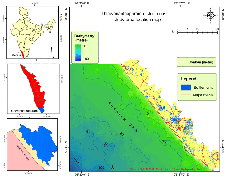
The coastal zone of the Thiruvananthapuram district of Kerala, India, covers a stretch of about 72 km extending seaward for 10 km from the coast. The geographical extent of the area is between a latitude of 8∘17′ and 8∘54′ N and a longitude of 76∘41′ and 77∘17′ E (Fig. 1). The coastal stretch is highly dynamic due to hydrodynamic forces such as waves, currents, tides, etc. The area has also undergone changes regarding near shore bathymetry and coastal landforms. Natural and anthropogenic activities have caused morphological instability in the landforms along the coast. Commercial activities, tourist sites, dense populations, and thick settlement are characteristic features of major locations along this coastal stretch. Along the coast, human settlements and properties are threatened due to severe coastal erosion. The study area enjoys a subtropical climate. It receives an average annual rainfall that varies between 826 and 1456 mm, and an annual mean temperature that ranges from 23.78 to 33.95 ∘C (Meteorological Centre, IMD, Thiruvananthapuram, 2017) (https://www.imdtvm.gov.in, last access: January 2017).
3.1 Data used
We used OLI data for determining pre-monsoon (March 2017) and post-monsoon (September 2017) suspended sediments. OLI provides the multispectral data for the visible and infrared range, and covers the entire Earth in 16 days. The OLI uses the push broom sensor with an 185 km cross-track field of view.
Shuttle radar topography mission is a research effort that obtained digital elevation models to generate a high-resolution digital topography database of the Earth. For extracting the bathymetry, we used a global relief model which is a composite model that incorporates a digital bathymetry model (DBM). SRTM30_PLUS (http://topex.ucsd.edu/WWW_html/srtm30_plus.html, last access: January 2017) consists of both a topography and a bathymetry model; therefore, it provides 30 arcsec (900 m) resolution data for land as well as for ocean, which is derived from depth sounding (SONAR) and satellite altimetry. Finally, the wind direction was derived from the ERA-Interim portal, provided by the ECMWF (European Centre for Medium-Range Weather Forecasts, 2017), which is an independent intergovernmental organization, based on a four-dimensional IFS (Cy31r2) system.
3.2 Conversion of digital number (DN) values to top of atmosphere (TOA) reflectance
Atmospheric correction was applied to determine the water-leaving reflectance (ratio of upwelling radiance just above the water surface and the solar downwelling irradiance) by eliminating the contribution of surface glint and atmospheric scattering from the estimated total reflectance. The total atmospheric reflectance was estimated as the sum of the molecular reflectance (Rayleigh reflectance), specular reflection of the sun, and the reflectance of aerosol, foam, and whitecaps. All of these parameters were determined from the metadata and field measurements, using an empirical relationship (Gordon and Wang, 1994). Solar radiation is totally absorbed by water in the near-infrared band. Thus, water-leaving radiance can be eliminated to directly estimate aerosol. Hence, medium to relatively high suspended particulate matter (SPM) concentrations can be better mapped using the near-infrared and red bands.
These raw data can be converted to TOA reflectance from the DN (Eq. 1) using rescaling factors and parameters found in the metadata file (MTL.txt), which is provided with the data. This can be carried out as follows:
where is the TOA planetary reflectance (without solar angle correction), Mp is the band-specific multiplicative rescaling factor, Ar is the band-specific additive rescaling factor, and Qcal is the quantized and calibrated standard product pixel values (DN).
Next, we corrected the using Eq. (2) for the solar angle:
where ρt is the TOA planetary reflectance, θSE is the local sun elevation angle, θSZ is the local solar zenith angle, and .
3.3 Molecular/Rayleigh reflectance correction
Most reflectance from air molecules and aerosols must be accurately modelled and removed from the observed signal. At-sensor total reflectance (Eq. 3) can be expressed as the following formula:
After the Rayleigh correction, ground surface + aerosol albedo ra can be determined as
where ρR is the Rayleigh reflectance, the extra terrestrial sun radiation is (π)(ES)(cos(θS))(dsol)exp[(−m)(τnet)],
θs and θv are the angle of solar zenith and sensor zenith, respectively, dsol is the eccentricity correction factor of the Earth's orbit, and TR is the Rayleigh atmospheric transmittance.
Tyu = Rayleigh transmittance for sensor
Tyd = Rayleigh transmittance for sun
where τRaylight is the Rayleigh optical depth, is the oxygen optical depth, τ is the optical depth, and SR is the Rayleigh spherical albedo.
Rayleigh reflectance (ρr) is calculated as follows:
where μs=cos of sun zenith, μv=cos of sensor zenith, ∅v is the sun azimuth, ∅s is the sensor azimuth, ρR1 is the single-scattering contribution, and τ is the atmospheric optical depth.
Sensor spectral response-based pre-computed radiative transfer simulations, solar and sensor viewing geometry, and ancillary information were used to estimate most of the components in the above equations. Rayleigh correction was executed by subtracting the Rayleigh reflectance value from the top of atmosphere reflectance as
3.4 Marine reflectance calculation
Aerosol reflectance (ε) over water pixels was derived from the ratio of reflectance in the chosen bands. ε, the proportion of the multiple-scattering aerosol reflectance, was constant over the study period. The value of ε was considered to be 1 for standard processing in the visual and near-infrared bands (Vanhellemont et al., 2014). A linear relation was established between marine reflectance and constant aerosol type (ε). Aerosol can be determined by the slope of the regression line (Neukermans et al., 2009) and the median ratio of the Rayleigh corrected reflectance in bands 4 and 5 (, ). Alpha, ∝, the ratio of oceanic reflectance was determined using the average resemblance spectrum for the band central wavelengths:
Gamma, γ is the fraction of diffused atmospheric transmittance in the two bands, which is calculated using the following equation (Eq. 8):
Then, the oceanic reflectance is calculated using and (Eq. 9):
3.5 Spectral analysis of the suspended sediments
The reflectance spectrum of an object is a graph of the radiation reflected to the incident wavelength and serves as a unique signature for the particular object. The water curve is characterized by high absorption in the near-infrared wavelength and beyond, whereas maximum reflectance is found in blue range of the spectrum. The spectral curve for the SSC is plotted for suspended particles in the ocean at a certain wavelength, after establishing the marine reflectance and correcting for aerosol in the data.
3.6 Extraction of suspended sediments and its validation
After obtaining the error free reflectance data, we proceeded with mapping the movement of suspended sediments during the pre-monsoon and post-monsoon seasons. Increments in red reflectance range in turbid water indicate the presence of sediments. We determined suspended solid matter using the single band (the red band) algorithm (Eq. 10) that was also used by Nechad et al. (2010):
where A=327.84 g m−3 and C=0.1708.
Using the above-mentioned method, we mapped the solid particles suspended near the shore (within 10 km) in order to explore the transportation of suspended particle along the coast during the pre-monsoon and post-monsoon seasons.
As previously stated, the single band algorithm, which was suitable for the study area, was used as a predictor for assessing the suspended sediments along the coast. The model was validated with samples collected within 5 km of the coast. The root mean square error (RMSE) was calculated (Eq. 11),
to examine the variation between the field-based predicted () data and the satellite-based observed (y) data values. This study used the concurrent satellite and ground-based data for better calibration.
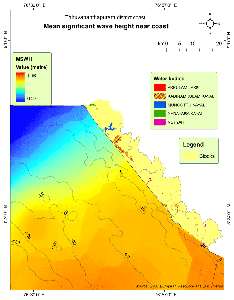
Sources of suspended sediments general consist of discharges from rivers, shore erosion, and the weathering of rocky shores. These sources control the creation of coastal headlands and provide source material to the physical, chemical, and biological inputs in the offshore region. The accumulation of suspended sediments in coastal regions changes the coastal morphology. The sediments near the shore are transported, instead of stably remaining in one place, due to the various hydrodynamic influences of the ocean, such as mean significant wave height (Fig. 2). Mean significant wave height can be calculated as the average height of the highest one-third of the measured waves (Eq. 12), which are N in number:
The individual wave height (Hm) is classified with highest wave being m=1 and the lowest wave being m=N. The average hight of one-third of the measured waves is used as it corresponds best with the visual observations of experienced mariners. It is evident from Fig. 2 that the mean significant wave height is high for the southern part of the study area, and decreases towards the north of the study region. Therefore, high wave energy has the potential to mix more sediments in the southern region of the study area compared to the lower energy areas; this is due to the fact that higher wave energy does not allow the sediments to be transported to other places.
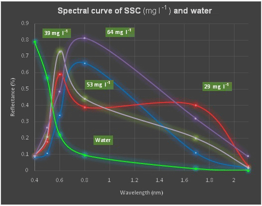
4.1 Spectral signature of water and SSC having different magnitudes
The reflectance curve (Fig. 3) is plotted between the wavelengths utilized and the detected suspended sediment reflectance from a 900 m2 area (at 30 m resolution). The reflectance variation of the surface water indicates the presence of suspended sediments in the offshore region (Fig. 3). We note that the regions with high suspended sediment concentrations have high reflectance at near-infrared wavelengths, and regions with comparatively lower suspended sediment concentrations have high reflectance in the red part of the spectrum. The areas with no suspended sediments show high reflectance in the blue region of the spectrum and total absorption at near-infrared wavelengths. Hence, the reflectance curve helps with the determination of the concentration of suspended sediments in the water.
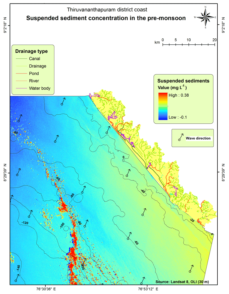
4.2 Monitoring of suspended sediments
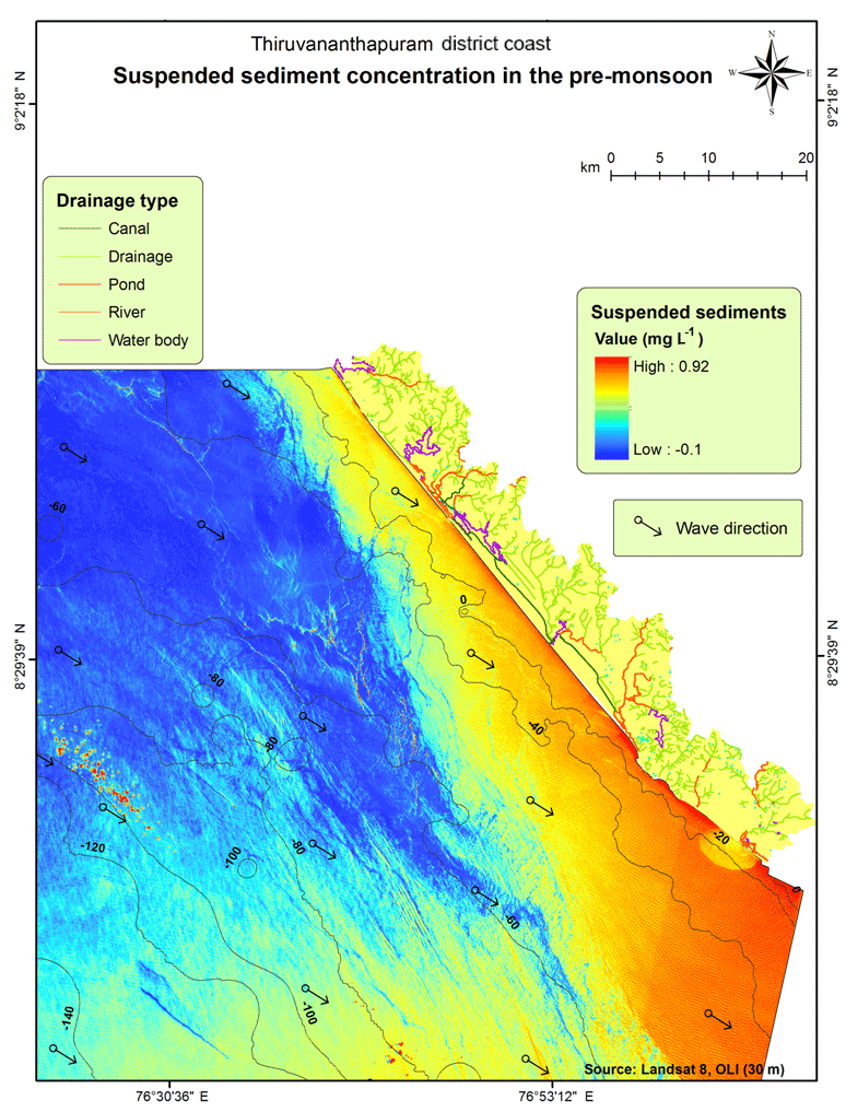
The northern part of study area experienced heavy deposition during the post-monsoon, as the suspended particles were swashed by fewer high energy waves; the dominant wave direction during this season was also conducive to deposition (Fig. 4). Whereas, in the pre-monsoon season, circulation of the sediments was found to occur in the lower part of the study area due to the dominate wave and current action along the shore (Fig. 5). Basically, a sediment particle will remain suspended when the vertical velocity of the fluid motion becomes greater than the settling velocity of the particle. Therefore, with respect to the wave field, the vertical motion must result from the combined effects of turbulence and wave orbital motion. Here another phenomenon also acts on the sediments – the gravity of the sediments suspended in the ocean – as the heavy sediments get deposited near shore, whereas the lighter sediments float. The wave directions in the pre-monsoon and post-monsoon periods are shown in Figs. 4 and 5, respectively. It was found that the SSC rapidly decreased with an increase in the distance (0–10 km) from the shoreline as well as an increase in the bathymetry level of 5–10 m. Furthermore, the effect of wave shoaling was deeper water is significantly less, which was found to cause a sparse distribution of sediment concentrations. Suspended sediment concentrations more than 5000 m from the shoreline and below a depth of 10–20 m, are rarely observed as measurement at these depths is not currently possible, which is one of the limitations of the optical data. The movement of SSCs indicates that SSCs have a positive correlation with wave direction and littoral current. We assigned weight to the layer based on the deposition along the shore. Most of the southern part of the study area was found to exhibit high concentrations of suspended matter during pre-monsoon and post-monsoon seasons, which were derived from the single band model with a very small RMS error, i.e. 0.19. The middle part of the study region was found to have cyclic SSCs, as it experienced seasonal erosion of the shore and deposition sediments near the beach. The northern most part of the study area was found have lower concentrations of suspended sediments during the pre-monsoon and post-monsoon seasons.
This paper explored the concentration and movement of suspended particles along the Thiruvananthapuram coast. The findings revealed that the sediment concentration decreased rapidly with an increase in the distance from the beach and the depth from the seabed. As the bathymetry increased, lower amounts of available sediments moved towards the shore, causing lower concentrations in the surface water. Waves, which are frequent phenomena, although at comparatively larger distances from one another in deeper water, caused a sparse distribution of sediments. Thus, sediments were concentrated at a lower depth in high bathymetry (≥10 m) and at distances of more than 2 km from the shoreline. This study found higher suspended sediment concentrations near the coast, particularly in surf zones and areas with water depths up to 50–100 m; however, these higher concentrations were observed to disappear with an increase in the bathymetry, as the phenomena of wave breaking and littoral current did not allow the suspended sediments move far from the coast.
This study provides interesting visions regarding monitoring the near-shore suspended sediments after radiometric and geometric corrections. Another prospect of this study is the analysis of factors affecting the suspended particles in near-shore and offshore areas. OLI (30 m) has a spectral range from 0.45 to 0.88 nm for the visible band in addition to the near-infrared band, which have demonstrated the best details for spectral response analysis. This analysis revealed that the high reflection in the near-infrared expressed the high concentration of SSCs, whilst the high reflection in the visible range expressed the lower concentration of suspended sediments. Suspended sediments moved north to south during the pre-monsoon and reversed their direction during post-monsoon season, under the influence of monsoon winds. Mapping the spatial distribution of suspended materials using remotely sensed data has the potential to aid in the management of coastal environment. Therefore, further study in this direction would aid the determination of the point and non-point sources of water bodies, which discharge into the ocean. Hence, remote sensing data could potentially be utilized as a tool for monitoring the sediments in the ocean.
The research data are available at https://www.imdtvm.gov.in/index.php?option=com_content&task=view&id=29&Itemid=43, https://dds.cr.usgs.gov/srtm/, and http://apps.ecmwf.int/datasets/data/interim-full-daily/levtype=sfc/.
HS, KS and BRT formulated the research work and processed the data; KS, PK, and BRT implemented the technique; and KS, PK, BSC, and PKJ discussed, validated, and designed the article.
The authors declare that they have no conflict of interest.
The authors are incredibly grateful to Pawan Kumar Chaudhary, Nguyen Hao Quang, and
Oliver Zielinski for their constructive comments and suggestions, which
helped to improve the overall quality of the present work. The Central Geomatics
Laboratory (CGL), the ESSO- National Centre for Earth Science Studies (NCESS),
and the Ministry of Earth Sciences Government of India are sincerely acknowledged for
their constant support.
Edited by:
Oliver Zielinski
Reviewed by: Pawan Kumar Chaudhary and Nguyen Hao Quang
Byers, A. C.: Soil loss and sediment transport during the storms and landslides of May 1988 in Ruhengeri prefecture, Rwanda, Nat. Hazards, 5, 279–292, 1992.
Curran, P. J. and Novo, E. M. M.: The relationship between suspended sediment concentration and remotely sensed spectral radiance: a review, J. Coast. Res., 4, 351–368, 1988.
European Centre for Medium-Range Weather Forecasts: ERA Interim, available at: https://www.ecmwf.int/ (last access: February 2017), 2018.
Gao, P.: Understanding watershed suspended sediment transport, Prog. Phys. Geogr., 32, 243–263, 2008.
Gordon, H. and Wang, M.: Retrieval of water-leaving radiance and aerosol optical thickness over the oceans with SeaWiFS: a preliminary algorithm, Appl. Optics, 33, 443–452, 1994.
Islam, M. R., Yamaguchi, Y., and Ogawa, K.: Suspended sediment in the Ganges and Brahmaputra River in Bangladesh: observation from TM and AVHRR data, Hydrol. Process., 15, 493–509, 2001.
Kaliraj, S. and Chandrasekar, N.: Spectral recognition techniques and MLC of IRS P6 LISS III image for coastal landforms extraction along South West Coast of Tamilnadu, India, Bonfring, Int. J. Adv. Image Process., 2, 01–07, 2012.
Kaliraj, S., Chandrasekar, N., and Magesh, N. S.: Impacts of wave energy and littoral currents on shoreline erosion/accretion along the south-west coast of Kanyakumari, Tamil Nadu using DSAS and geospatial technology, Environ. Earth Sci., 8, 239–253, https://doi.org/10.1007/s12665-013-2845-6, 2013a.
Kaliraj, S., Chandrasekar, N., and Magesh, N. S.: Evaluation of coastal erosion and accretion processes along the southwest coast of Kanyakumari, Tamil Nadu using geospatial techniques, Arab. J. Geosci., 71, 4523–4542, https://doi.org/10.1007/s12517-013-1216-7, 2013b.
Katlane, R., Nechad, B., Ruddick, K., and Zargouni, F.: Optical remote sensing of turbidity and total suspended matter in the Gulf of Gabes, Arab. J. Geosci., 6, 1527–1535, 2013.
Kisi, O.: Modeling discharge-suspended sediment relationship using least square support vector machine, J. Hydrol., 456–457, 110–120, 2012.
Kronvang, B., Laubel, A., and Grant, R.: Suspended Sediment and Particulate Phosphorus Transport and Delivery Pathways in an Arable Catchment, Gelbaek Stream, Denmark, Hydrol. Process., 11, 627–642, 1997.
Marcus, W. A. and Fonstad, M. A.: Remote sensing of rivers: the emergence of a subdiscipline in the river sciences, Earth Surf. Proc. Land., 35, 1867–1872, 2010.
Meteorological Center: IMD, Thiruvananthapuram, available at: https://www.imdtvm.gov.in (last access: January 2017), 2018.
Moore, G. K.: Satellite remote sensing of water turbidity/Sonde de télémesure par satellite de la turbidité de l'eau, Hydrolog. Sci. Bull., 25, 407–421, 1980.
Nechad, B., Ruddick, K., and Park, Y.: Calibration and validation of a generic multi-sensor algorithm for mapping of total suspended matter in turbid waters, Remote Sens. Environ., 114, 854–866, 2010.
Neukermans, G., Ruddick, K., Bernard, E., Ramon, D., Nechad, B., and Deschamps, P .Y.: Mapping total suspended matter from geostationary satellites: a feasibility study with SEVIRI in the Southern North Sea, Opt. Express, 17, 14029–14052, 2009.
Ontowirjo, B., Paris, R., and Mano, A.: Modeling of coastal erosion and sediment deposition during the 2004 Indian Ocean tsunami in Lhok Nga, Sumatra, Indonesia, Nat. Hazards, 65, 1967–1979, 2013.
Panwar, S., Agarwal, V., and Chakrapani, G. J.: Morphometric and sediment source characterization of the Alaknanda river basin, headwaters of river Ganga, India, Nat. Hazards, 87, 1649–1671, 1–23, 2017.
Qu, L.: Remote sensing suspended sediment concentration in the Yellow River, PhD dissertation paper 383, University of Connecticut, available at: http://digitalcommons.uconn.edu/dissertations/383/, last access: December 2014.
Rawat, Pradeep K., Tiwari, P. C., Pant, C. C., Sharama, A. K., and Pant, P. D.: Modelling of stream run-off and sediment output for erosion hazard assessment in Lesser Himalaya: need for sustainable land use plan using remote sensing and GIS: a case study, Nat. Hazards, 59, 1277–1297, 2011.
Sinha, P. C., Guliani, Pragya, Jena, G. K., Rao, A. D., Dube, S. K., Chatterjee, A. K., and Murty, T.: A Breadth Averaged Numerical Model for Suspended Sediment Transport in Hooghly Estuary, East Coast of India, Nat. Hazards, 32, 239–255, 2004.
Tassan, S.: A procedure to determine the particulate content of shallow water from Thematic Mapper data, Int. J. Remote Sens., 19, 557–562, 1998.
Vanhellemont, Q., Neukermans, G., and Ruddick, K.: Synergy between polar-orbiting and geostationary sensors: Remote sensing of the ocean at high spatial and high temporal resolution, Remote Sens. Environ., 146, 49–62, 2014.
Wang, J. J. and Lu, X. X.: Estimation of suspended sediment concentrations using Terra MODIS: an example from the Lower Yangtze River, China, Sci. Total Environ., 408, 1131–1138, 2010.
Warrick, J. A., Merters, L. A. K., Siegel, D. A., and Mackenzie, C.: Estimating suspended sediment concentrations in turbid coastal waters of the Santa Barbara Channel with SeaWiFS, Int. J. Remote Sens., 25, 1995–2002, 2004.
Whitelock, C. H., Witte, W. G., Taly, T. A., Morris, W. D., Usry, J. W., and Poole, L. R.: Research for reliable quantification of water sediment concentrations from multispectral scanner remote sensing data, NASA-TM-82372, US National Aeronautics and Space Administration, Langley Research Center, Hampton, VA, 243–255, 1981.
Yanjiao, W., Feng, Y., Peiqun, Z., and Wenjie, D.: Experimental research on quantitative inversion models of suspended sediment concentration using remote sensing technology, Chinese Geogr. Sci., 17, 243–249, 2007.
Zhang, Y., Pulliainen, J., Koponen, S., and Hallikainen, M.: Water quality retrievals from combined Landsat TM data and ERS-2 SAR data in the Gulf of Finland, IEEE T. Geosci. Remote, 41, 622–629, 2003.