the Creative Commons Attribution 4.0 License.
the Creative Commons Attribution 4.0 License.
 | 15 Oct 2018
Wind-driven transport of fresh shelf water into the upper 30 m of the Labrador Sea
Eleanor Frajka-Williams
The Labrador Sea is one of a small number of deep convection sites in the North Atlantic that contribute to the meridional overturning circulation. Buoyancy is lost from surface waters during winter, allowing the formation of dense deep water. During the last few decades, mass loss from the Greenland ice sheet has accelerated, releasing freshwater into the high-latitude North Atlantic. This and the enhanced Arctic freshwater export in recent years have the potential to add buoyancy to surface waters, slowing or suppressing convection in the Labrador Sea. However, the impact of freshwater on convection is dependent on whether or not it can escape the shallow, topographically trapped boundary currents encircling the Labrador Sea. Previous studies have estimated the transport of freshwater into the central Labrador Sea by focusing on the role of eddies. Here, we use a Lagrangian approach by tracking particles in a global, eddy-permitting () ocean model to examine where and when freshwater in the surface 30 m enters the Labrador Sea basin. We find that 60 % of the total freshwater in the top 100 m enters the basin in the top 30 m along the eastern side. The year-to-year variability in freshwater transport from the shelves to the central Labrador Sea, as found by the model trajectories in the top 30 m, is dominated by wind-driven Ekman transport rather than eddies transporting freshwater into the basin along the northeast.


In the Labrador Sea deep mixing and the formation of deep dense water are possible due to intense winter heat loss that removes surface buoyancy (Clarke and Gascard, 1984; Lazier, 1973; Pickart et al., 2002). The so-formed Labrador Sea Water (LSW) joins the deep western boundary current (DWBC) and is transported south as part of the Atlantic meridional overturning circulation (AMOC) (Pickart and Smethie, 1998; Rhein et al., 2002; Talley and McCartney, 1982). Overall, the upper Labrador Sea is characterized by relatively salty Atlantic water offshore and cold freshwater in the boundary currents over the shelves. Offshore of the boundary currents, in the salty basin, less cooling is required to cause static instabilities in winter, making the Labrador Sea one of the prime regions for deep convection (Lazier and Wright, 1993; Marshall and Schott, 1999).
Freshening of the Labrador Sea surface water, in combination with weaker air–sea fluxes, could reduce or eliminate convection due to the increase in surface buoyancy. In fact, freshening periods of varying intensity are not uncommon in the Labrador Sea (Houghton and Visbeck, 2002) due to its proximity to the fresh Arctic outflow and melt from the Greenland ice sheet. An example of a complete shutdown of deep water formation due to anomalous surface buoyancy and weak air–sea fluxes was observed during the Great Salinity Anomaly (GSA) in the 1970s (Dickson et al., 1988; Gelderloos et al., 2012). Convection later resumed due to increasing air–sea fluxes and the advection of saltier water (Gelderloos et al., 2012). Increased freshwater input in the North Atlantic over the last few decades (Bamber et al., 2012) could result in a similar situation and again decrease the deep water formation rate. Model simulations indicate that predicted rates of freshening in the North Atlantic will cause a 20 % change in the strength of the AMOC (Häkkinen, 1999; Jahn and Holland, 2013; Manabe and Stouffer, 1995; Robson et al., 2014). Until 2005 a freshening signal was not detectable in the upper Labrador Sea (Yashayaev, 2007). However, more recent studies, using ocean observations from Argo floats and ship-based hydrography, show that the surface layer of the North Atlantic, including the Labrador Sea, has freshened, while deep densities have decreased (Robson et al., 2014; Yashayaev et al., 2015). Despite this trend in reduced salinity, deep convection and the formation of a new LSW class was observed in 2014–2016 (Yashayaev and Loder, 2016).
Early “hosing experiments” were performed in coarse-resolution numerical models to simulate large amounts of freshwater released during paleoclimate events. These simulations showed that freshwater spread uniformly across the entire North Atlantic and Labrador Sea (Weaver et al., 1994). Higher-resolution models suggest, however, that additional freshwater in the Labrador Sea may be confined to the shelf region (Myers, 2005) where it would have less influence on the properties of the convection region. While model resolution is crucial in the Labrador Sea (Chanut et al., 2008; Gelderloos et al., 2012; Myers, 2005), some features seem to be present regardless of the resolution. An increase in freshwater in the convection region was observed in models with resolutions of , , and (Dukhovskoy et al., 2015). The pathways of freshwater into the region of deep convection were similar in the three models – entering the region of convection mainly from the north and the east – but the amount differed between the models. Additionally, the study suggests that freshwater signals would likely be obscured by the increased salinity of the Atlantic water entering the region at the same time.
On seasonal timescales, freshwater is observed to enter the basin in a small pulse in the spring and a second, larger pulse in the fall (Schmidt and Send, 2007). The first freshwater peak is attributed to the Labrador Current and the second, larger peak to the West Greenland Current. This is consistent with Lilly et al. (2003), who identify the West Greenland Current as the primary source of freshening in the Labrador Sea basin. Additional freshwater enters the Labrador Sea from Davis Strait and Hudson Strait and joins the Labrador Current. Some evidence points to instabilities in the Labrador Current that could lead to the advection of freshwater into the basin (Cooke et al., 2014; LeBlond, 1982). Using a model, Cooke et al. (2014) argue that the instabilities could indicate a direct connection between the Labrador Current and central basin salinities. Such a connection would further support the idea of a Labrador Current source to the fall freshening in the central Labrador Sea, but the dynamics are not further discussed and the coarse model allows freshwater to leave the Labrador Current more easily than might be the case in the real ocean.
In the past, studies have concentrated on eddies in the top hundreds of meters as the main mechanism by which heat and freshwater are imported into the basin. Eddies originating at the boundary current can carry warm and buoyant water (Gelderloos et al., 2012; Jong et al., 2014; Lilly et al., 2003) and have been associated with seasonal freshening (Chanut et al., 2008; Hátún et al., 2007; Katsman et al., 2004). Eddies with a core of Irminger Sea Water, termed Irminger Rings, are shed from the boundary current near the northeast corner of the basin (around 64∘ N, 54∘ W) (Gelderloos et al., 2012; Lilly et al., 2003). When assuming that 30 eddies are shed from the boundary current each year (as suggested by Lilly et al., 2003), up to 50 %–80 % of the wintertime heat loss to the atmosphere can be balanced by eddies advecting heat (Katsman et al., 2004; Lilly et al., 2003). This accounts for only about 50 % of the seasonal freshening in the basin (Hátún et al., 2007; Lilly et al., 2003; Straneo, 2001). Hence, there is an unresolved discrepancy between the advection of freshwater by eddies and that required to explain the annual freshwater gain in the basin. Observational studies may underestimate the number of eddies due to the coarse resolution of altimetry data relative to eddy size, while models are likely to misrepresent the advection due to eddies because of problems with mixed layer depths and grid size. In fact, an eddy-resolving ice–ocean model that, according to the authors, performed better in the Labrador Sea than previous models, found that near-surface freshwater advection into the Labrador Sea basin increased (Kawasakim and Hasumi, 2014). However, this and previous studies failed to explain all of the seasonal freshwater fluxes by eddies alone. To explain the missing seasonal freshwater fluxes, other dynamics, for example Ekman transport, might also have to be considered.
Every year, substantial buoyancy is lost from the Labrador Sea basin during the wintertime convection. This buoyancy is replenished by surface heat fluxes and lateral buoyancy fluxes (Straneo, 2001), which have both a time-varying and a mean component. Here we focus on these aspects using a numerical model to better understand the role Ekman transport might have in advecting freshwater into the Labrador Sea basin in the top 30 m. In this study we use Lagrangian trajectories in a high-resolution () numerical model to investigate how, when, and where surface freshwater from boundary currents enters the central Labrador Sea, in particular the relative importance of eddies vs. wind in allowing freshwater to escape the shelves and enter the basin. In Sect. 2, we describe the model and methods. In Sect. 3, we outline the typical pattern of shelf-edge crossings and their salinity and origin. In Sect. 4, we consider the variability of crossings and its relations to eddy and wind activity in the region. We conclude in Sect. 5 with a summary and discussion.
We use output from a numerical model to compute offline Lagrangian trajectories of water particles. Trajectories are ideally suited to identify the pathway and origins of water parcels with associated temperatures and salinities. The latter are key to our focus on processes driving the movement of water from the shelves to the central basin. In the following, we describe the numerical model and compare velocity and hydrography to observations (Sect. 2.1). We then give an overview of the particle-tracking software (ARIANE) and detail particle releases (Sect. 2.2 and 2.3), as well as explaining the criteria for a “crossing” from shelf to basin (Sect. 2.4). A large part of this work focuses on the origin of particles and in Sect. 2.5 we define the regions of origin.
2.1 NEMO data
For this study, output from the high-resolution global ocean circulation model Nucleus for European Model of the Ocean ORCA v3.6 ORCA0083-N06 (NEMO N06 from here on) is utilized (Madec, 2016; Marzocchi et al., 2015; Moat et al., 2016). The model has a horizontal resolution of with a tripolar grid (one pole in Canada, one in Russia, and one on the South Pole) to avoid numerical instability associated with convergence of the meridians at the geographic North Pole. Resolution is coarsest at the Equator (9.26 km) and increases to about 4 km in the Labrador Sea. This allows the model to resolve some mesoscale eddies. Smaller features are parameterized.
The model has 75 vertical levels that are finer near the surface (about 1 m) and increase to 250 m at the bottom. The bottom topography is derived from the 1 min resolution ETOPO bathymetry field of the National Geophysical Data Center (http://www.ngdc.noaa.gov/mgg/global/global.html, last access: December 2017) and is merged with satellite-based bathymetry. Model output is produced every 5 days. Lateral mixing varies horizontally according to a bi-Laplacian operator with a horizontal eddy viscosity of 3×10¹¹ m4 s−1. Vertical mixing at sub-grid scales was parameterized using a turbulent kinetic energy closure model (Madec, 2016). Background vertical eddy viscosity and diffusivity are 10−4 m2 s−1 and 10−5 m2 s−1, respectively. The model is forced by the Drakkar surface forcing data set v5.2. developed by the Drakkar consortium (http://www.drakkar-ocean.eu/, last access: December 2017) supplying air temperature, winds, humidity, surface radiative heat fluxes, and precipitation. It is used for the period 1958–2012, with a horizontal resolution of 1.125∘ (Brodeau et al., 2010; Dussin et al., 2014). Precipitation and downward shortwave and longwave radiation are taken from the CORE forcing data set Large and Yeager (2004), while wind, air humidity, and air temperature are derived from the ERA-Interim reanalysis fields. Surface momentum in the model is applied directly as a wind stress vector using daily mean wind stress. To prevent unrealistic salinity drifts in the model due to deficiencies in the freshwater forcing, the sea surface freshwater fluxes are relaxed toward climatologies by 33.3 mm day−1 psu−1, corresponding to a relaxation timescale of 365 days. The subsequent analysis does not attempt to calculate any freshwater budgets or compare model salinities to observations. Instead we focus on pathways of fresh vs. salty water into the basin as well as month-to-month and interannual changes in the freshwater that is transported to the basin within the model. The sea ice module used is from the Louvain-la-Neuve sea ice model (LIM2) (Timmerman et al., 2005). For each model cell, the model uses the ice fraction to compute the ice–ocean fluxes combined with the air–sea fluxes to provide the surface ocean fluxes. No icebergs are implemented in this version.
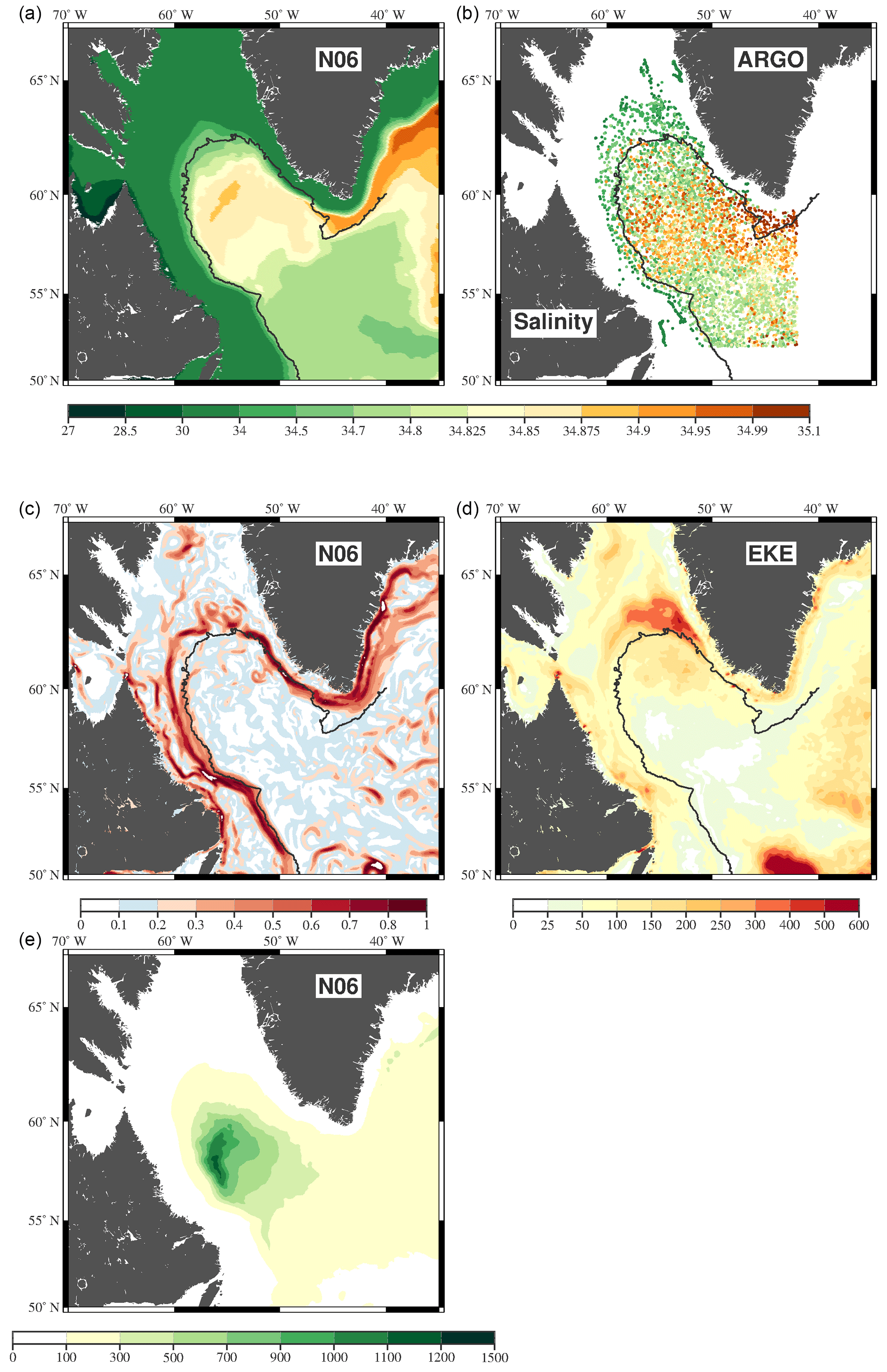
Figure 1(a) Mean salinity in the top 100 m from NEMO-N06. (b) The same as (a) but from Argo data. (c) Speed (m s−1) and (d) mean EKE (cm2 s−2) derived from the NEMO-N06 model of the top 100 m. (e) Mean wintertime (December–March) mixed layer depths (m) from NEMO-N06. All means are calculated for the period of 2002–2009.
No-slip conditions are implemented at the lateral boundaries, except in the Labrador Sea where a region of partial slip is applied. This is done to favor the breakup of the West Greenland Current into eddies (as observations have suggested). The ocean in the model is bounded by complex coastlines, bottom topography, and an air–sea interface. The major flux between the continental margins and the ocean is a mass exchange of freshwater through river runoff (taken from the 12-month climatological data of Dia and Trenberth, 2002), modifying the surface salinity. There are no fluxes of heat and salt across boundaries between solid earth and ocean, but the ocean exchanges momentum with the earth through frictional processes. Initial conditions for the model were taken from Levitus et al. (1998) with the exception of high latitudes and Mediterranean regions where PHC2.1 (Steele et al., 2001) and MEDATLAS (Jourdan et al., 1998) are used, respectively. The model is run for the period of 1958–2012. Here we analyze the time period of 1990–2009, for which eddies and wave fields (Rossby waves) had ample time to spin up.
2.2 Model evaluation
To improve the NEMO run, changes were incorporated in the N06 run to better represent boundary currents, interannual variability, and the depth of mixed layers. These changes were (1) more consistent wind forcing reaching back to 1958 (more information at http://www.drakkar-ocean.eu/forcing-the-ocean/the-making-of-the-drakkar-forcing-set-dfs5, last access: December 2017), (2) steeper topography along the Greenland coast, and (3) use of a partial slip along western Greenland (Quartly et al., 2013). The changes in topography together with the partial slip condition promotes the formation of eddies in this region, resulting in improved salinity and velocity fields (Chanut et al., 2008) (Fig. 1). The N06 simulation was previously used in other studies of the North Atlantic, one of which found that the model is able to represent the variability of heat transport at 26.5∘ N (Moat et al., 2016).
In the NEMO N06 model, the deepest winter mixed layers in the Labrador Sea basin are located in the western basin, consistent with observations (Pickart et al., 2002; Schulze et al., 2016; Våge et al., 2008), (Fig. 1). The model tends to overestimate the mixed layers in the Labrador Sea basin (Courtois et al., 2017), but the agreement of the mixed layer depths and location indicates that the boundary current and the advection of freshwater and heat into the basin are represented well. Without this representation the basin stratification would be weaker and mixing would be stronger. This in turn would result in mixed layers in the wrong location that are much deeper than in the observations. The relationship between fresh shelf water and mixed layers in the basin can be seen in a previous model study (McGeehan and Maslowski, 2011). That study failed to represent the low-salinity water along the western coast of Greenland and produced unrealistic deep convection in the wrong area of the Labrador Sea.
The mean NEMO N06 surface salinities in the Labrador Sea are shown in Fig. 1 together with data from Argo floats in the region (see http://www.argo.ucsd.edu/, last access: December 2016, for information about these data). Argo data are generally not available on the shelves where water is shallower than 1000 m (with some exceptions) but the deep basin properties are well observed. Both the surface salinities in NEMO and from Argo data show freshest water (below 34.8) in the coastal regions. At Cape Farewell (southern tip of Greenland), salinities are high: 34.9 in NEMO and above 34.99 in the Argo data. The salinity of the basin is 34.85 in NEMO with a saltier region in the northwest (34.875–34.9) and a fresher region in the northeast (34.8–34.5). A similar salinity distribution can be found in the Argo data. The saltiest region is in the western basin with salinities around 34.9. The freshwater in the northeast extends further into the basin but with salinities around 34.5–34.8. While there are some differences, both the model and observations show increased salinities in the western Labrador Sea, as well as a band of slightly lower salinities extending across the Labrador Sea. This band joins the high salinities in the southeastern Labrador Sea. Seasonal cycles of the basin-averaged salinities in NEMO and from Argo data are in phase with peak salinities in February–March and the freshest water in September (not shown). Modeled salinities are overestimated by around 0.1 between November and June. The NEMO N06 model shows a strong West Greenland Current (WGC) and Labrador Current (LC), as well as flow from Baffin Bay and Hudson Strait (Fig. 1). The region around 62∘ N and 52∘ W, described as the region of high eddy kinetic energy (EKE) in many studies (e.g., Brandt et al., 2004; Chanut et al., 2008; Eden and Böning, 2002; Lilly et al., 2003), is characterized in NEMO N06 by an energetic WGC and the formation of eddies. Along the coast of the Labrador Peninsula, the flow is separated into two currents, a coastal flow and the main branch of the Labrador Current. The coastal current is mainly fed by outflow from Hudson Strait and is separated from the Labrador Sea basin (Han et al., 2008). The flux between the Labrador Sea and Baffin Bay experiences a strong seasonal cycle in NEMO that is consistent with hydrographic observations in this region (Curry et al., 2014; Myers, 2005; Rykova et al., 2015).
Along the east coast of Greenland, the EGC is also split into a coastal and main branch. Such coastal flow is consistent with observations (Sutherland and Pickart, 2008). Luo et al. (2016) show a similar flow pattern in their model study, with current speeds of the WGC and LC of up to 1 m s−1, but their data show very little eddy activity in the northeast. A model agrees with our N06 model and shows a strong and steady WGC that becomes unstable around 62∘ N and 52∘ W (Böning et al., 2016).
The region of high EKE in the northeast corner of the Labrador Sea basin has been described in many studies. For example, using merged along-track TOPEX/Poseidon and ERS data for 1997–2001, Brandt et al. (2004) found the region of largest EKE at 62∘ N, inshore of the 2500 m isobath, with maximum values as high as 700 cm2 s−2. The EKE reached values of 300 cm2 s−2 inside the basin (offshore of the 2500 m isobath) close to the northeast corner, consistent with Chanut et al. (2008), Katsman et al. (2004), and Lilly et al. (2003). The EKE calculated from the NEMO data has very similar values with maximum EKE in the same location as shown by Brandt et al. (2004). In particular, the region of the highest EKE is located inshore of the 2500 m isobath at around 62∘ N, with values of up to 600 cm2 s−2. Inside the basin, the northeast is characterized by EKE values of up to 200 cm2 s−2. The highest values of EKE in the model used by Luo et al. (2016) are consistent with the location of the highest EKE values in NEMO. Altimetry data, on the other hand, did not show elevated EKE inside the basin (Brandt et al., 2004). Brandt et al. (2004) further observed that the EKE in the WGC is on average more than 300 cm2 s−2 higher than in the central LS and that the minimum–maximum EKE in the WGC and the basin occurs in September–January. This is also true for the NEMO N06 data.
2.3 ARIANE and experiment setup
The offline Lagrangian tool ARIANE is used to track particles using velocity fields output from the NEMO model. ARIANE is available at http://www.univ-brest.fr/lpo/ariane (last access: April 2015) and described in detail by Blanke and Raynaud (1997) and Blanke et al. (1999). For each 5-day time step of the model the trajectories are analytically solved, respecting the mass conservation of the model within each grid cell. For this study, particles were released every 10 days at 264 points in the Labrador Sea basin over the 20-year period 1990–2009 (Fig. 2). To determine the impact of wind vs. eddies on surface freshwater fluxes into the Labrador Sea, we released particles at three different depths (0, 15, and 30 m). This resulted in 28 512 particle releases each year, for a total of 570 240 particles over the 20 years. Each particle is tracked backwards for 1 year. These particles provide a statistical description of water pathways in the Labrador Sea.
2.4 Particles crossing into the basin
We refer to the Labrador Sea basin as the region that is offshore of the 2500 m isobath. This basin is encircled by the boundary currents that on average are centered at this isobath (Fig. 1c). While the particles were released in the basin and tracked backwards, we will refer to their trajectories as forward in time (i.e., particles enter the basin to end up at their release point). A particle is considered to have entered the basin if it crossed the 2500 m isobath from shallow into deeper water within the top 30 m of the water column. If a particle crossed the isobath multiple times, only the last time before reaching its release point was considered. In addition, the particle has to be at least 50 km away from the 2500 m isobath to be considered as within the basin. This criterion ensures that the particle has left the boundary current completely. The 50 km threshold was determined by averaging the velocities of the basin as a function of distance from the 2500 m isobath (not shown). Average velocities exceed 0.25 m s−1 within 20 km of the 2500 m isobath but decrease to 0.1 m s−1 at a distance of 50 km. There is little to no influence of the boundary currents beyond this distance and velocities remain constant at 0.1 m s−1.
Note that particles are only considered if they crossed into the basin within the top 30 m. From 1990 to 2009, a total of 570 240 particles were released, of which 230 147 (40 %) entered the basin within the top 30 m (Table 1). Additionally, we only considered crossings that occur within 7 months of the particle release. This is the case for a total of 205 929 particles. A randomly chosen ensemble of particle trajectories in this category is shown in Fig. 3. The 7-month cutoff allows the seasonal cycle to be resolved, but the results presented below are not strongly sensitive to the choice of a cutoff time. Of the remaining 323 084 trajectories that are not categorized as crossings according to the above criteria, 1657 crossed below 30 m and 15 352 were initialized in the basin and remained there during their 1-year lifetime (Table 1). The largest number of particles (56 %) entered the basin from the south but never crossed the 2500 m isobath.
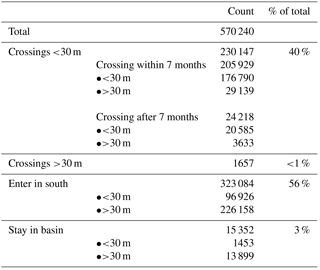
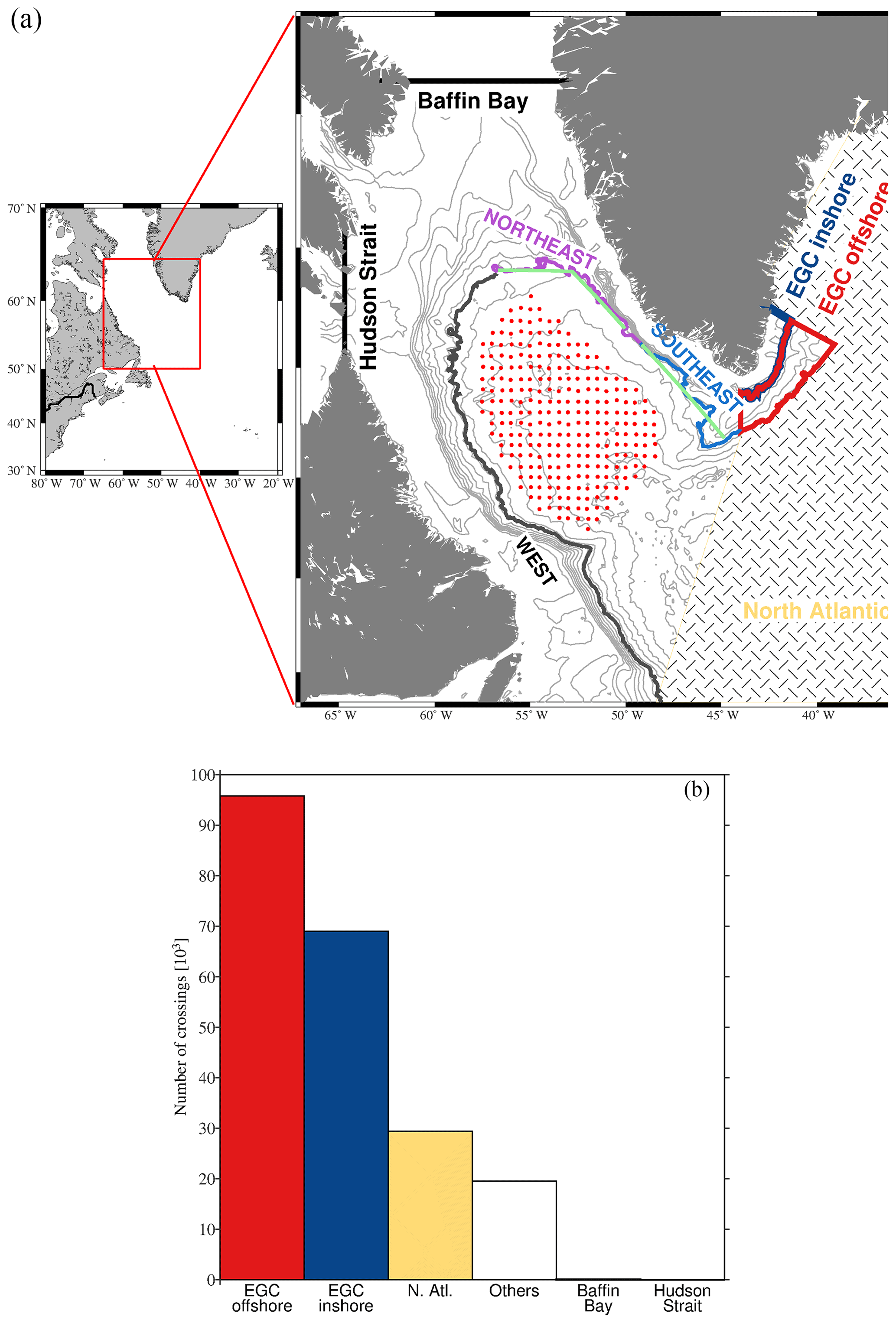
Figure 2(a) The location of the Labrador Sea (left) and a zoomed-in view of the Labrador Sea on the right. The topography is shown in gray contours, spaced in 500 m intervals. The thick contour shows the 2500 m isobath and is referred to as the boundary between shelf and basin in the text. The areas referred to in the study as southeast and northeast are shown in blue and purple, respectively. Red dots denote the release positions of the particles in this study. The five regions referred to as the origin of water are also shown here. The East Greenland Current (EGC) inshore and offshore region are shown as the blue and red box, respectively. Baffin Bay and Hudson Strait are shown as black sections and the North Atlantic region as the yellow line and structured region. (b) The number of crossings per origin. East Greenland offshore (red), East Greenland inshore (blue), other regions in the North Atlantic (yellow), unidentified origins (no color), Baffin Bay and Hudson Strait (black). The light green sections show the sections across which Ekman transport is calculated.
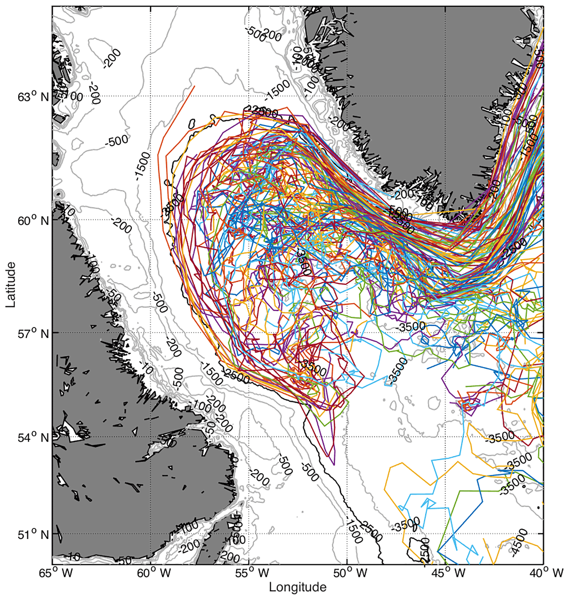
Figure 3Trajectories of 0.01 % of the 205 929 trajectories that entered the basin. The trajectories were chosen randomly and are shown in a different color each. Bathymetry is contoured in gray at 500 m intervals with the 2500 m isobaths in black.
2.5 Regions and water sources
The boundary between shelf and basin – the 2500 m isobath – is split into three areas: southeast, northeast, and west (Fig. 2). Particles crossing into the basin via these three sections are traced to their source. We consider five sources: Hudson Strait, Baffin Bay, East Greenland Current (EGC) inshore, EGC offshore, and water from other sources in the North Atlantic (also referred to as North Atlantic water; Fig. 2). The EGC inshore and offshore sources at the East Greenland coast are separated by the 1000 m isobath. This isobath coincides with a strong surface salinity gradient of 0.6 between the fresh inshore water and saltier offshore water (not shown). If a particle passed through either the EGC inshore or offshore regions at any point during its lifetime it is considered to have its origin in the EGC. A particle is considered to originate from Hudson Bay if at any point it was located west of 65∘ W. Similarly, every particle that passed through the region west of Greenland and north of 65∘ N has its origin in Baffin Bay. All other particles must originate elsewhere and are of North Atlantic origin.
A total of 80 % of the particles that entered the Labrador Sea basin originate in the EGC (both inshore and offshore; Fig. 2). Specifically, 95 810 (46.5 %) of the 205 929 particles originated in the offshore section of the EGC; 69 028 (33.5 %) originated in the inshore EGC (hence from the shelf). A much smaller number (29 406 or 14 %) entered the Labrador Sea basin from elsewhere in the North Atlantic. During the 20 years considered here, only 153 particles (1 %) originated in Baffin Bay and 4 in Hudson Bay. Because of this small number (compared to the number of crossings from the other sources), Baffin Bay and Hudson Bay are not considered in the results from here on. Due to the 1-year lifetime of the particles, 5.5 % (11 528) of particles that crossed into the basin did not originate in any of these five regions. Hence, at the end of their lifetime they were located outside the basin but had not left the Labrador Sea.
2.6 Probability of crossings
Below we present the number of crossings as the probability of particles entering the basin in a certain region or during a specific time period (e.g., monthly or yearly). The probability is calculated by dividing the number of crossings in a certain region or within a certain time period by the total number of crossings.
2.7 Ekman transport
To calculate the expected Ekman transport for a homogeneous ocean into the basin we use the ERA-Interim reanalysis 10 m wind product for 1990–2009. Daily winds are interpolated onto the southeast and northeast (Fig. 2) and the along- and across-velocity components are projected onto the respective section to be along (τ∥) and across the section (τ⊥). In this way, the Ekman transport across the section is given by
where τ is the mean wind stress along the section (calculated following Large and Pond, 1980), f the Coriolis force, and ρ the mean water density.
2.8 Error analysis
Errors on the number of crossings and salinity are calculated using a Monte Carlo approach. For the calculation of the error, a 90 % subset of the variable (number of crossings and salinity) is selected randomly with replacement, and the mean of the variable across the subset is calculated. The process is repeated 5000 times, after which the distribution of the estimated mean can be used to determine 95 % confidence intervals. The error evaluates the robustness of our estimates using a reduced number of particles but does not address any uncertainties associated with model shortcomings in salinity or velocity fields.
In this section, we discuss the geography of crossings identified by the ARIANE particles in the NEMO N06 model run. In general, the highest probability of particles crossing into the basin occurs in the southeast and northeast of the Labrador Sea (Fig. 4). In the west, the probability is about 4 times smaller. It is worth noting that the probability is slightly elevated south of 57∘ N (sections IV and V in Fig. 5). The southeast has the highest probability of particles entering the basin (sections I and II) with average salinities of 34.98. That is 0.04 higher than the average salinities of particles crossing in the northeast (34.94). Low-salinity water crosses in the northeast (sections II and III). This combined with the high probability of crossings results in a high likelihood of freshwater entering the basin here. Crossings in the southeast, on the other hand, do not supply any freshwater to the basin overall due to the high salinities of the crossing particles. Hence, the model output shows two distinct pathways of water into the basin: salty water enters in the southeast and freshwater in the northeast.

Figure 4The probability of crossings per 100 km along the boundary is indicated by the size of the circles, with larger circles indicating a larger probability. The color shows the mean salinity of the crossings at each section.
3.1 Crossings by water sources
To analyze the origin of the water (fresh and salty) that entered the basin in the northeast and southeast, we consider water originating in the EGC (inshore and offshore) as well as water from other regions in the North Atlantic separately. Water from the offshore EGC source is most likely to enter the basin in the southeast, a short distance downstream from Cape Farewell (Fig. 5). These particles are salty with an average of 34.97. The main pathway of EGC inshore water into the basin is about 200 km farther north along the boundary. Compared to the EGC offshore water, the water here is much fresher with salinities as low as 34.91. Water with origin elsewhere in the North Atlantic primarily enters the basin a short distance from Cape Farewell via the southeast (section I). The water is about 0.04 fresher than the EGC offshore water that also crosses the boundary primarily at this location. Farther along the 2500 m isobath, the salinities of the water from all three sources are comparable and the probability of crossings decreases to close to zero (sections III–VI). For all three water sources, the speed at which particles cross into the basin is comparable (not shown).
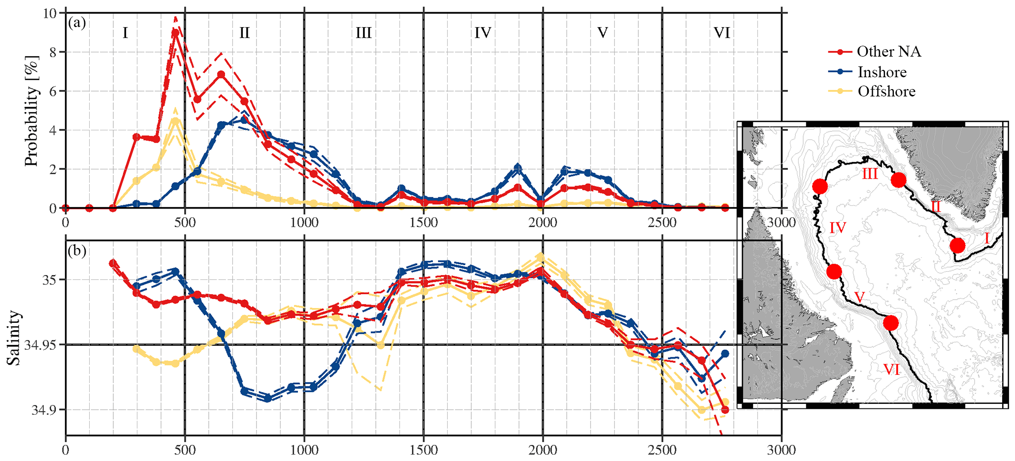
Figure 5(a) The probability of crossings per 100 km section (solid line) and the estimated error (dashed line). (b) The average salinity of the crossing particles at each 100 km section (solid line) and the associated error (dashed lines). The black horizontal line shows the reference salinity of 34.95 that is used to calculate the freshwater flux. In both panels the vertical lines correspond to the location of the red circles on the map to help orient the reader geographically. Red lines show the EGC offshore water, blue the EGC inshore water, and yellow the water from other regions of the North Atlantic.
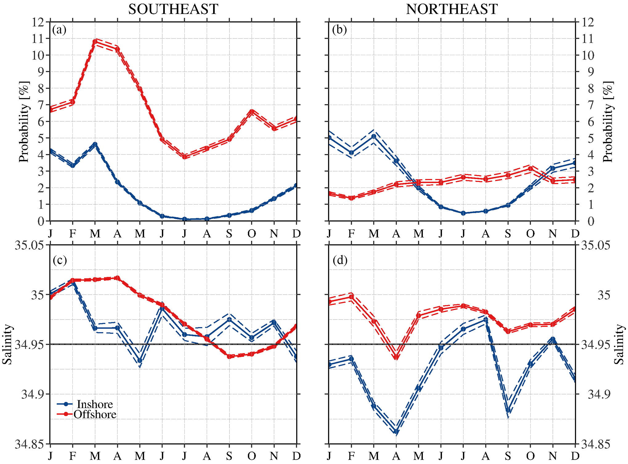
Figure 6(a) Seasonal cycle of the probability of particles entering the basin in the southeast and (b) northeast (see Fig. 2 for the location of the regions). Seasonal cycle of salinity for particles crossing in the (c) southeast and (d) northeast. In all panels, the colors show the sources of the water: blue lines shows water from the EGC inshore region and red the water from the EGC offshore region. The dashed lines show the associated errors.
In summary, a large amount of EGC offshore water crosses into the basin in the southeast and results in an influx of relatively salty water to the basin. The EGC inshore water enters farther north and brings fresher water to the basin. Compared to the high probability that water enters along the eastern side of the basin, the crossings along the western side are negligible. Additionally, in our study the contribution to freshwater fluxes from the water of other North Atlantic sources is small as well. Therefore, we focus on water originating in the EGC inshore and offshore and entering the Labrador Sea basin along the eastern side.

Figure 7The 3-monthly mean of eddy kinetic energy (color, cm2 s−2) and wind (vectors, m s−1) in the Labrador Sea, 1990–2009, for (a) December–February, (b) March–May, (c) June–August, and (d) September–November. The white boxes in (a) show the regions over which EKE is averaged in Fig. 8. The white lines in (b) show the sections across which Ekman transport is calculated.
In the following section, we identify the seasonal and interannual variability of particle crossings in the model run. To quantify if water is fresh or salty we will refer to a reference salinity of 34.95, which is the average salinity of the top 30 m of the basin from 1990 to 2009. Note that this study and the following conclusions are for the top 30 m only.
4.1 Seasonality of crossings
We divide the crossing particles according to their origin (EGC inshore or offshore) and the location at which they enter the basin (southeast or northeast) to investigate their seasonality. In the southeast, the probability of particles of EGC origin entering the basin is greatest in March (Fig. 6). However, the probability of EGC offshore water crossing is twice as high as the probability of inshore water crossing (10.8 %±0.2 % and 4.6 %±0.1 %, respectively). In addition to the high probabilities in March, probabilities of inshore water crossing are high in January (4.2 %±0.1 %). In summer the crossing probability is about half that of the one in March for both inshore and offshore water. During the minimum in July, offshore water crosses with a likelihood of 3.8 %±0.1 % and inshore water with a probability of 0.1 %±0.02 %. In the northeast, the probability of EGC offshore water crossing into the basin is low, varying from 1.3 % in February to 3.2 % in October. The seasonal cycle of the inshore crossings, however, is similar (in timing and magnitude) to the southeast region, with maximum probabilities in January and March and a minimum in the summer. Inshore water is about twice as likely as offshore water to enter during the time of convection (November–April), 5 %±0.2 % vs. 1.8 %±0.1 %, respectively. In the summer, inshore water crossings drop to almost zero, while offshore water keeps entering the basin with a probability of 3.5 %±0.1 %. In the southeast, EGC inshore and offshore water entering the basin is saltier than 34.95, with the exception of May and December. In the northeast, the seasonal cycle of inshore water crossings is characterized by two pulses of freshwater, one in December–April and a second, shorter pulse in September. The two pulses can be identified by the salinity decreasing to around 0.08 below the reference salinity (in April and September). The EGC offshore water also freshens during these two periods, but this freshening is much weaker and salinities remain close to the reference salinities. The high probability of inshore freshwater entering the basin in the spring is balanced by the high probability of high-salinity water entering along the southeast section and results in the fall freshening being stronger than the spring freshening.
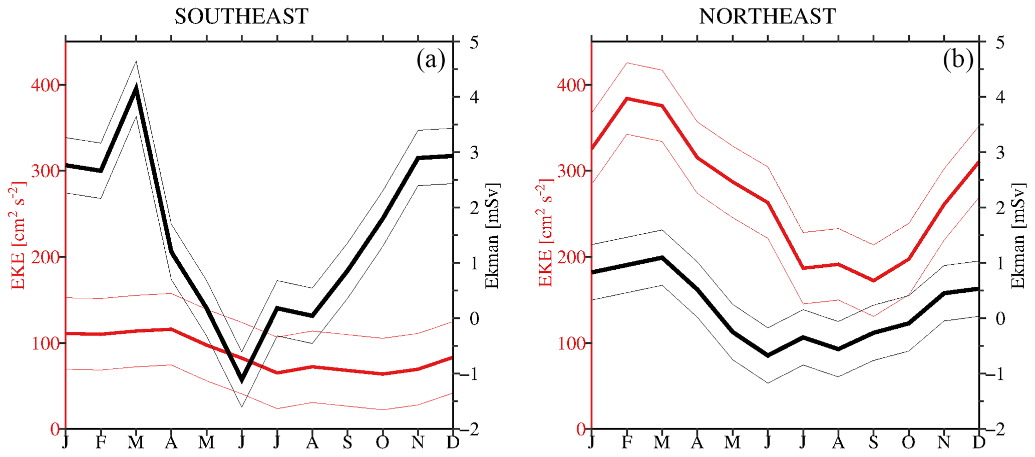
Figure 8(a) The seasonal cycle of EKE (red line) and Ekman transport (black line) (1990–2009) in the southeast (see the white box and section in Fig. 7). The thin lines show the associated standard deviation. (b) Same but for the northeast.
4.1.1 Seasonal role of winds and eddies
The 3-monthly composites of EKE and wind speeds show that the northeast portion of the Labrador Sea experiences EKE of 500 cm2 s−2 in the spring and winter, 400 cm2 s−2 in the summer, and 200 cm2 s−2 in the fall. Winds are predominantly northwesterly (Fig. 7) and result in a southwestward Ekman transport, which, for the Greenland side of the Labrador Sea, is in the offshore direction. The Ekman transport is highest in the winter, lower in the spring, and nearly zero in the summer.
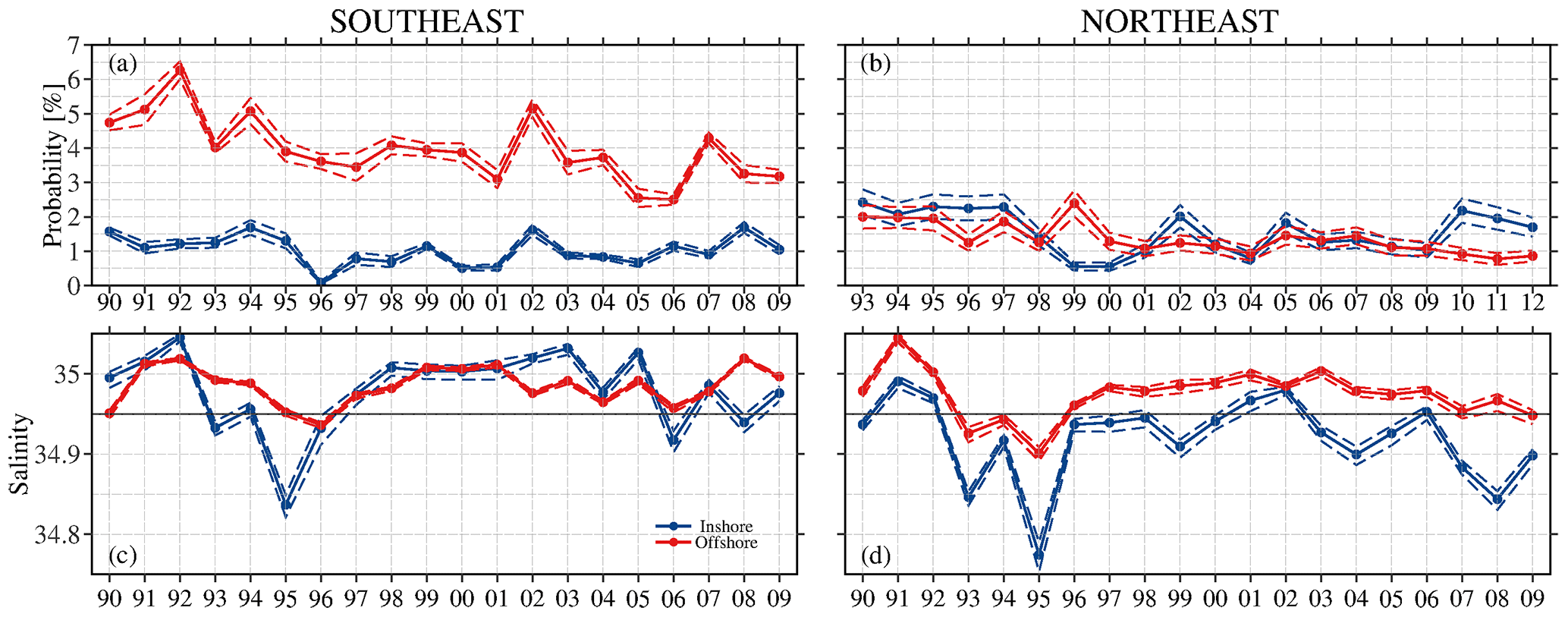
Figure 9The probability of water entering the basin in the (a) northeast and (b) southeast. The salinities of particles crossing in (c) the northeast and (d) the southeast. The colors refer to the water's origin: blue shows the EGC inshore water, red the EGC offshore water. The doted lines show the estimated errors.
The seasonal cycle of EKE near the southeast section is weak, with values around 80 cm2 s−2 all year (Fig. 8). In the northeast, on the other hand, EKE values are much higher, with an average of nearly 300 cm2 s−2 and a seasonal amplitude of 200 cm2 s−2. The maximum EKE is observed in February and March. Ekman transport into the basin in the upper 30 m is strongest in the southeast, with peak values of around 4 mSv in March and a minimum of −1 mSv (transport out of the basin) in June. (Note that this is the overall water transport due to the winds, not the freshwater transport.) In the southeast, the peak of EGC inshore and offshore crossings coincides with the peak of the Ekman transport. In the northeast, however, the peak of EKE and Ekman transport coincides only with the peak of inshore crossings. Due to the similar timing of the seasonal EKE and wind cycles, we cannot use the timing to distinguish between their potential roles in transporting water from the shelves into the basin. In order to separate their effects, the interannual variability of the number of crossings, EKE, and Ekman transport is evaluated.
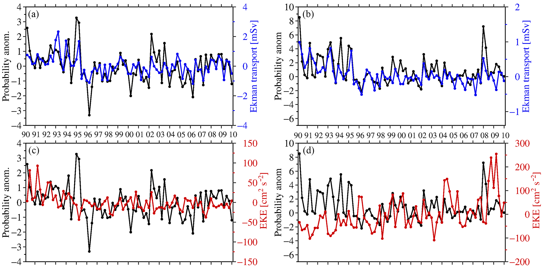
Figure 10Three-monthly anomaly of the crossing probability (black line) and Ekman transport (blue line) in the southeast (a) and northeast (b). Panels (c, d): same but for the crossing anomaly (black line) and EKE anomaly (red line). Note that axis ranges change for the different regions.
4.2 Interannual variability of crossings
The annual average probability of crossings and their average salinities are determined for the southeast and northeast sections (Fig. 9). Throughout the entire 20 years, offshore water is twice as likely to enter the basin in the upper 30 m via the southeast compared to inshore water. The inshore water crossings show little variability and no apparent long-term trend throughout the 20-year period, while there is a decrease in the amount of offshore water that enters the basin. In the northeast, the probabilities of EGC inshore and offshore waters entering the basin are comparable. In both regions, the offshore water transports mainly salty water (relative to the reference salinity), while the inshore water is relatively salty in the southeast and fresher in the northeast. Salinities during 1993–1995 are anomalously low along the entire eastern boundary. Other periods of elevated freshwater fluxes occurred in 1999, 2004, and 2007–2009 when salinities of the inshore water fell below the reference salinity. During the entire 20 years, the EGC offshore water was the main source of salty water and entered in the southeast. Due to the low number of crossings, the EGC inshore water did not contribute significantly to fresh or salty water in the basin. In the northeast, where both sources were equally likely to enter the basin, EGC inshore water caused large freshwater fluxes in 1993–1995, 1999, 2004, and 2007–2009 due to its low salinities.
4.2.1 Interannual role of winds and eddies
We compare the interannual crossing probabilities to the anomalies of the Ekman transport and EKE. In particular, 3-month-averaged time series of EKE, Ekman transport, and the probability of crossings in the southeast and northeast are constructed. To consider variations beyond the seasonal cycle, the mean seasonal cycle for 1990–2009 is removed and the resulting anomalies are compared to the crossing probabilities (Fig. 10). The time series for EKE and Ekman transport are correlated with the probability anomaly using the Pearson method (Emery and Thomson, 2001). When considering only the top 30 m, we find that anomalies of the crossing probabilities in the southeast are not significantly correlated with the EKE anomaly in this region (Table 2). The crossing probabilities do, however, have a low but significant correlation with the Ekman transport (r=0.43). This relationship is more pronounced in the northeast where the variability of the crossings is strongly correlated with the variability in the Ekman transport (r=0.73). In other words, in the northeast the variability in the Ekman transport explains the majority of the variability in the number of crossing particles. In the NEMO model used here, EKE and hence eddies do not play a role in this relationship (correlation of r=0.05). One possible exception to this may be in the northeast during the period 1998–2002, when there appears to be a period of transient correlation between crossing probability and EKE. When repeating this calculation separately for the inshore and offshore crossings, only the probability of the inshore water crossing is significantly correlated with the Ekman transport (not shown). Furthermore, the correlation between EGC inshore water and the Ekman transport is stronger in the northeast (r=0.72) than the southeast (r=0.54), though both are significant.
Table 2Correlation of the number of crossings in the southeast–northeast and the EKE and Ekman transport in the same region. The table shows the r value of each correlation, printed in bold if the correlation is significant within 99 % confident levels.
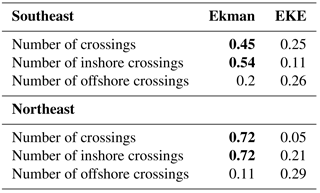
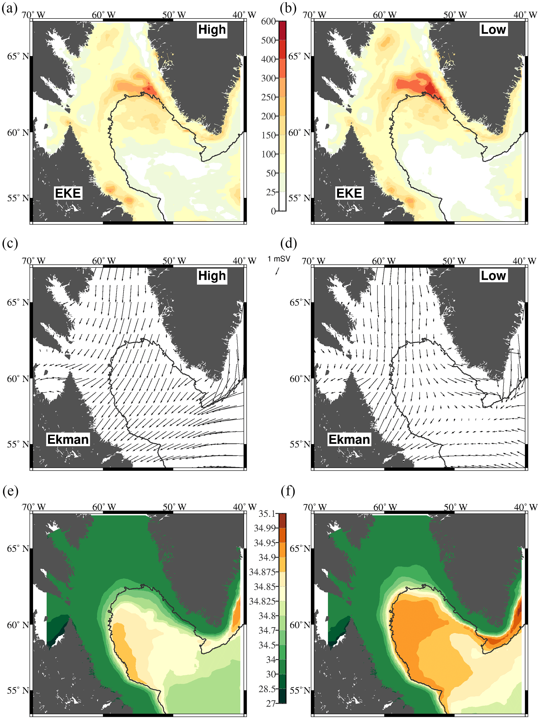
Figure 11(a, b) The mean surface EKE (cm2 s−2) during months with an anomalously high and low number of crossings. (c, d) Same as (a, b) but for the Ekman transport. (e, f) Same as (a, b) but for the model salinities of the top 30 m.
For a spatial view of the different conditions during times with high vs. low crossings, maps of EKE, Ekman transport, and the mean salinity of the Labrador Sea are calculated (Fig. 11). In particular, the maps are comprised of months when the probability of crossings in the southeast and northeast is outside of a 2 standard deviation envelope. At times when crossing probabilities are high, the EKE in the northeast is weak and the Ekman transport across the eastern side of the basin is stronger compared to times with anomalously low crossings. Additionally, the surface salinities on the Greenland shelves and the central Labrador Sea basin are 0.2 fresher when the probability of crossings is high. The WGC at Cape Farewell is also fresher in this scenario.
The following pattern emerges: during times with anomalously high crossings, the EKE in the northeast, just inshore and adjacent to the 2500 m isobath, is on average 100 cm2 s−2 lower than during months with a low probability of crossings. The northeast region just inside the 2500 m isobath, on the other hand, has similar EKE values for both scenarios. Much larger differences are found in the Ekman transport. During times of anomalously low transport, winds force water into the basin along the northern boundary, but the Ekman transport is parallel to the eastern boundary and results in weak cross-shelf Ekman transport here. This is accompanied by higher than average salinities on the shelves. When the number of crossings is high, however, the Ekman transport is strong and perpendicular to the eastern boundary, allowing the water to spread away from the shelf into the basin. This leads to an overall freshening of the basin.
We use the ocean model NEMO and the Lagrangian particle-tracking tool ARIANE to assess the major routes and mechanisms of freshwater in the Labrador Sea basin. This is important in understanding how freshwater released from the Greenland ice sheet or the Arctic may influence the region of deep convection in the Labrador Sea. Investigating the temporal variability of the cross-shelf movement of water demonstrates the importance of Ekman transport to the cross-shelf transport in the upper 30 m. In particular, we considered the role of Ekman transport and eddy fluxes (approximated by eddy kinetic energy) for the exchange between the boundary and basin in the upper 30 m.
Lagrangian trajectories suggest that in this configuration of the NEMO model with the given forcing, 80 % of water entering the basin in the top 30 m each year originates in the EGC. It reaches the Labrador Sea via the WGC before crossing into the basin along the eastern boundary. In comparison, water originating from other regions such as Baffin Bay and Hudson Strait is negligible. There are possible shortcomings in how the circulation in these regions is represented in the model and it would be worth verifying with observational data that there is no additional pathway for freshwater from these sources to the Labrador Sea basin. We find the dominant pathway of water particles from the boundary to the central basin to be in the northeast. Wind-driven transport plays an important role in forcing the interannual, and possibly the seasonal, variability of cross-shelf exchange in the model. Higher-resolution models that better resolve the eddies in the Labrador Sea will be needed to fully understand the role eddies play in transporting freshwater to the basin in this region.
Seasonally, the largest number of crossings is observed in the spring, but fluxes into the basin continue at a lower rate throughout the year. This is consistent with previous observationally based estimates using a budget framework showing continuous fluxes of water into the basin (Straneo, 2001). Freshwater is advected into the basin in two pulses in the spring and in the fall, as was also observed by Schmidt and Send (2007) and Straneo (2001). Due to the different methods applied in the studies (e.g., deeper surface layers and different reference salinities) and the saltier model used here, the absolute magnitudes of the freshening pulses are not explicitly compared. However, the results are consistent in the timing of the freshening. One of the unique benefits of a Lagrangian approach is the ability to determine the statistical source of the water entering the basin. We investigate the origin of the freshwater that enters the basin, finding that the water from the inshore region of the EGC enters the Labrador Sea in the northeast (Fig. 5d). This water is responsible for both the spring and fall freshening pulses. At the same time of the spring freshening, large amounts of salty EGC offshore water enter the basin in the southeast (Fig. 5c). This counteracts and weakens the overall spring freshening observed in the basin. The fall pulse (September–October), on the other hand, is the result of a combination of relatively low-salinity water from the EGC offshore source and fresh EGC inshore water. The two water masses enter the basin in two different regions, the EGC offshore water in the southeast and the EGC inshore water in the northeast.
Our results show that water entering the Labrador Sea basin in the surface layer was freshest in the mid-1990s, with other maxima in 1999, the early 2000s, and mid-2000. The freshening in the mid-1990s is likely to be related to the freshening observed by Häkkinen (1999), with the freshest waters located on the shelves. Several other years stand out as well, such as 1999, 2003–2004, and 2007–2008. The water responsible for these freshening periods originates in the inshore part of the EGC. A surface freshening signal in 2007–2008 was found in observations and the model. This is also the year in which deep convection was observed again after a long period of absence (Våge et al., 2008). It is not clear what exactly caused the freshening periods since the NAO is neither strongly positive nor strongly negative and there is no obvious increase in Greenland runoff at these times.
Due to the remarkably high correlation between the Ekman transport and crossing probability, we suggest that wind forcing plays the primary role in the variability of freshwater transport near the surface and allows fresh shelf water to enter the basin in the top 30 m. This conclusion is consistent with model results presented by Luo et al. (2016). In summary, as water rounds Cape Farewell and enters the Labrador Sea, large amounts of offshore water cross into the basin. In the upper 30 m, the inshore water spreads away from the coast, off the shelf, and towards the basin due to Ekman transport. The offshore water enters the basin due to other mechanisms (not addressed in this study) and hence the number of crossings of this water is not significantly correlated with the Ekman transport.
While the Lagrangian approach is useful in investigating the timing, relative numbers of crossings, and salinities of crossings, it cannot be directly related to net transport across a section. For a quick comparison, we calculate the freshwater fluxes due to Ekman transport directly from the model data by using the wind and mean model salinities of the top 30 m across the eastern sections: the Ekman transport is responsible for a mean inflow of 1.5 mSv of freshwater. To estimate eddy fluxes across the same sections, we consider , where v is the total volume flow, the time mean, and v′ a deviation from the time mean and hence the volume flux due to eddy fluxes. This is done for the southeast and northeast sections and multiplied by the freshwater relative to the reference salinity Sref=34.95. The mean freshwater flux due to the eddy fluxes is 0.2 mSv. This is an order of magnitude lower than the freshwater fluxes due to Ekman transport. Repeating this calculation for the upper 100 m (a more common choice of the surface layer in the Labrador Sea; Schmidt and Send, 2007; Schulze et al., 2016; Straneo, 2001), we find that the combined freshwater transport to the basin due to Ekman and eddy fluxes is 2.4 mSv. This means that the freshwater flux in the top 30 m makes up 60 % of the total freshwater flux over the top 100 m. Of this, more than half is due to Ekman transport. When dividing the freshwater flux of the top 100 m into Ekman transport and eddy fluxes, the Ekman transport alone accounts for more than 60 % of the total 2.4 mSv. Eddy fluxes become more important (60 % vs. 40 %) only when extending the calculation to 200 m.
Two novel results emerge from this study. First, in the upper 30 m two seasonally occurring freshwater pulses can be identified in the model and are traced to the EGC. The inshore water is the main source of freshening in the top 30 m of the basin, seasonally and interannually. This means that Arctic meltwater and runoff from Greenland have a large influence on the freshwater input in the surface layer of the central Labrador basin. In light of the changing climate, this could reduce the formation of LSW with the potential for further reduction in the overturning circulation (Robson et al., 2014). Second, we show that Ekman transport plays a significant role in the advection of water to the upper 30 m of the basin. Previous studies concentrated on determining how large a role eddies play in the restratification of the Labrador Sea, but in a region where the freshest water is concentrated at the surface and winds are strong, the surface Ekman transport cannot be neglected.
The NEMO model is available at https://www.nemo-ocean.eu/ (Madec, 2016). Ariane can be found at http://stockage.univ-brest.fr/~grima/Ariane/ (Blanke and Raynaud, 1997).
The authors declare that they have no conflict of interest.
This work was supported by the University of Southampton Graduate School.
Edited by: Matthew Hecht
Reviewed by: two anonymous referees
Bamber, J., van den Boreke, M., Etterna, J., and Lenaerts, J.: Recent large increase in freshwater fluxes from Greenland into the North Atlantic, Geophys. Res. Lett., 39, L19501, https://doi.org/10.1029/2012GL052552, 2012. a
Blanke, B. and Raynaud, S.: Kinematics of the Pacific Equatorial Undercurrent: An Eulerian and Lagrangian approach from CM results, J. Phys. Oceanogr., 27, 1038–1053, 1997. a, b
Blanke, B., Arhan, M., Madec, G., and Roche, S.: Warm water paths in the equatorial Atlantic as diagnosed with a general circulation model, J. Phys. Oceanogr., 29, 2753–2768, 1999. a
Böning, C., Behrens, E., Biastoch, A., Getzlaff, K., and Bamber, J.: Emerging impact of Greenland meltwater on deepwater formation in the North Atlantic Ocean, Nature, 9, 523–527, 2016. a
Brandt, P., Schott, A., Funk, A., and Martins, C.: Seasonal to interannual variability of the eddy field in the Labrador Sea from satellite altimetry, J. Geophys. Res., 109, C02028, https://doi.org/10.1029/2002JC001551, 2004. a, b, c, d, e
Brodeau, L., Barnier, B., Treguier, A., Penduff, T., and Gulev, S.: An ERA40-based atmospheric forcing for global ocean circulation models, Ocean Model., 31, 88–104, 2010. a
Chanut, J., Barnier, B., Large, W., Debreu, L., Penduff, T., Molines, J., and Mathiot, P.: Mesoscale eddies in the Labrador Sea and their contribution to convection and restratification, J. Phys. Oceanogr., 38, 1617–1643, 2008. a, b, c, d, e
Clarke, R. and Gascard, J.-C.: The formation of Labrador Sea Water. Part I: Large-scale processes, J. Phys. Oceanogr., 13, 1764–1778, 1984. a
Cooke, M., Demirov, E., and Zhu, J.: A model study of the relationship between sea-ice variability and surface and intermediate water mass properties in the Labrador Sea, Atmosphere Ocean, 52, 142–154, 2014. a, b
Courtois, P., Hu, X., Pennelly, C., Spence, P., and Myers, P.: Mixed layer depth calculation in deep convection regions in ocean numerical models, Ocean Model., 120, 60–78, 2017. a
Curry, B., Lee, C., Petrie, B., Moritz, R., and Kwok, R.: Multiyear volume, liquid freshwater, and sea ice transports through Davis Strait, J. Phys. Oceanogr., 44, 1244–1266, 2014. a
Dia, A. and Trenberth, K.: Estimates of freshwater discharge from continents: Latitudinal and seasonal variations, J. Hydrometeor., 3, 660–687, 2002. a
Dickson, R., Meincke, J., Malmberg, S., and Lee, A. J.: The Great Salinity Anomaly in the Northern North Atlantic 1968–1982, Progr. Oceanogr., 20, 103–151, 1988. a
Dukhovskoy, D., Myers, P., Platov, G., Timmerman, M.-L., Curry, B., Bamber, J. L., Chassignet, E., Hu, X., Lee, C., and Somaville, R.: Greenland freshwater pathways in the sub-Arctic Seas from model experiments with passive tracers, J. Geophys. Res., 121, 877–907, 2015. a
Dussin, R., Barnier, B., and Brodeau, L.: The making of Drakkar forcing set DFS5, DRAKKAR/MyOcean Rep. 05-10-14, LGGE, Grenoble, France, 2014. a
Eden, C. and Böning, C.: Sources of Eddy Kinetic Energy in the Labrador Sea, J. Phys. Oceanogr., 32, 3346–3363, 2002. a
Gelderloos, R., Straneo, F., and Katsman, C.: The Mechanism behind the temporary shutdown of deep convection in the Labrador Sea: Lessons from the Great Salinity Anomaly Year 1968–71, J. Climate, 25, 6743–6755, 2012. a, b, c, d, e
Häkkinen, S.: A simulation of thermohaline effects of a Great Salinity Anomaly, J. Climate, 12, 1781–1795, 1999. a, b
Han, G., Lu, Z., Wang, Z., Helbig, J., Chen, N., and de Young, B.: Seasonal variability of the Labrador Current and shelf circulation of Newfoundland, J. Geophys. Res., 113, C12012, https://doi.org/10.1029/2009JC006091, 2008. a
Hátún, H., Eriksen, C., and Rhines, P. B.: Buoyant eddies entering the Labrador Sea observed with gliders and altimetry, J. Phys. Oceanogr., 37, 2838–2854, 2007. a, b
Houghton, R. and Visbeck, M.: Quasi-decadal salinity fluctuations in the Labrador Sea, J. Phys. Oceanogr., 32, 687–701, 2002. a
Jahn, A. and Holland, M.: Implications of Arctic sea ice changes for North Atlantic deep convection and the meridional overturning circulation in CCSM4-CMIP5 simulations, Geophys. Res. Lett., 40, 1206–1211, 2013. a
Jong, M. D., Bower, A., and Furey, H.: Two years of observations of warm-core anticyclones in the Labrador Sea and their seasonal cycle in heat and salt stratification, J. Phys. Oceanogr., 44, 427–444, 2014. a
Jourdan, D., Balopoulos, E., Garcia-Fernandez, M., and Maillard, C.: Objective analysis of temperature and salinity historical data set over the mediterranean basin, Oceans'98, 1, 82–87, 1998. a
Katsman, C., Spall, M., and Pickart, P.: Boundary current eddies and their role in the restratification of the Labrador Sea, J. Phys. Oceanogr., 34, 1967–1983, 2004. a, b, c
Kawasaki, T. and Hasumi, H.: Effect of freshwater from the West Greenland Current on the winter deep convection in the Labrador Sea, Ocean Model., 75, 51–64, 2014. a
Large, W. and Pond, S.: Open Ocean Momentum Flux Measurements in Moderate to Strong Winds, J. Phys. Oceanogr., 11, 324–336, 1980. a
Large, W. and Yeager, S.: Diurnal to decadal global forcing for ocean and sea-ice models: The data set and flux climatologies, NCAR Technical Note, National Center for Atmospheric Research, 11, 324–336, 2004. a
Lazier, J.: The renewal of Labrador Sea Water, Deep-Sea Res., 20, 341–353, 1973. a
Lazier, J. and Wright, D.: Annual velocity variations in the Labrador Current, J. Phys. Oceanogr., 23, 659–678, 1993. a
LeBlond, P.: Satellite observations of the Labrador Current undulations, Atmosphere Ocean, 20, 129–142, 1982. a
Lilly, J., Rhines, P., Schott, F., Lavender, K., Lazier, J., Send, U., and D'Asaro, E.: Observations of the Labrador Sea eddy field, Progr. Oceanogr., 59, 75–176, 2003. a, b, c, d, e, f, g, h
Luo, H., Castelao, R., Rennermalm, A. K., Tedesco, M., Bracco, A., Yager, P., and Mote, T. L.: Oceanic transport of surface meltwater from the southern Greenland ice sheet, Nature, 9, 528–533, 2016. a, b, c
Madec G. and the NEMO team: Note du Pole de modelisation de l'Institut Pierre-Simon Laplace No 27, https://www.nemo-ocean.eu/wp-content/uploads/NEMO_book.pdf, last access: October 2018, 2016. a, b, c
Manabe, S. and Stouffer, R.: Simulation of abrupt climate change induced by freshwater input to the North Atlantic Ocean, Lett. Nature, 378, 165–167, 1995. a
Marshall, J. and Schott, F.: Open-ocean convection: Observations, theory, and models, Rev. Geophys., 37, 1–64, 1999. a
Marzocchi, A., Hirschi, J.-M., Holiday, N., Cunningham, S., Blaker, A., and Coward, A.: The North Atlantic subpolar circulation in an eddy-resolving global ocean model, J. Mar. Sys., 142, 126–143, 2015. a
McGeehan, T. and Maslowski, W.: Impact of shelf-basin freshwater transport on deep convection in the western Labrador Sea, J. Phys. Oceanogr., 41, https://doi.org/10.1175/JPO-D-11-01.1, 2011. a
Moat, B., Josey, S., Sinha, B., Blaker, A., Smeed, D., McCarthy, G., Johns, W., Hirshi, J.-M., Frajka-Williams, E., Rayner, D., Ducjez, A., and Coward, A.: Major variations in subtropical North Atlantic heat transport at short (5 day) timescales and their causes, J. Geophys. Res., 121, 3237–3249, 2016. a, b
Myers, P.: Impact of freshwater from the Canadian Arctic Archipelago on Labrador Sea Water formation, Geophys. Res. Lett., 32, L06605, https://doi.org/10.1029/2004GL022082, 2005. a, b, c
Pickart, R. and Smethie, W.: Temporal evolution of the deep western boundary current where it enters the sub-tropical domain: Evidence from tracer data, Deep-Sea Res., 45, 1053–1083, 1998. a
Pickart, R., Torres, D., and Clarke, R.: Hydrography of the Labrador Sea during Active Convection, J. Phys. Oceanogr., 32, 428–457, 2002. a, b
Quartly, G., de Cuevas, B., and Coward, A.: Mozambique Channel eddies in GCMs: A question of resolution and slippage, Ocean Model., 63, 56–67, 2013. a
Rhein, M., Fischer, J., Smethie, W., Smythe-Wright, D., Weiss, R., Mertens, C., Min, D.-H., Fleischmann, U., and Putzka, A.: Labrador Sea Water: Pathways, CFC inventory and formation rates, J. Phys. Oceanogr., 32, 648–665, 2002. a
Robson, J., Hodson, D., Hawkins, E., and Sutton, R.: Atlantic overturning in decline?, Nature, 7, 2–3, 2014. a, b, c
Rykova, T., Straneo, F., and Bower, A.: Seasonal and interannual variability of the West Greenland Current System in the Labrador Sea in 1993–2008, J. Geophys. Res., 120, 1318–1332, 2015. a
Schmidt, S. and Send, U.: Origin and composition of seasonal Labrador Sea freshwater, J. Phys. Oceanogr., 37, 1445–1454, 2007. a, b, c
Schulze, L., Pickart, R., and Moore, G.: Atmospheric forcing during active convection in the Labrador Sea and its impact on mixed layer depth, J. Geophys. Res., 121, 6978–6992, 2016. a, b
Steele, M., Morley, R., and Ermold, W.: PHC: A global ocean hydrography with a high quality Arctic Ocean, J. Climate, 14, 2079–2087, 2001. a
Straneo, F.: Heat and Freshwater Transport through the Central Labrador Sea, J. Phys. Oceanogr., 36, 606–628, 2001. a, b, c, d, e
Sutherland, D. and Pickart, R.: The East Greenland Coastal Current: Structure, variability and forcing, Progr. Oceanogr., 78, 58–77, 2008. a
Talley, L. and McCartney, M.: Distribution and circulation of Labrador Sea Water, J. Phys. Oceanogr., 12, 1189–1205, 1982. a
Emery, W. J. and Thomson, R. E. (Eds.): Data Analysis Methods in Physical Oceanography, Elsevier Science, 371–567, https://doi.org/10.1016/B978-044450756-3/50006-X, 2001. a
Timmerman, A., Goossee, H., Madec, G., Fichefet, T., Ethe, C., and Dulire, V.: On the representation of high latitude processes in the ORCA-LIM global coupled sea-ice ocean model, Ocean Model., 8, 175–201, 2005. a
Våge, K., Pickart, R., Thierry, V., Reverdin, G., Lee, C., Petrie, B., Agnew, T., Wong, A., and Ribergaard, M.: Surprising return of deep convection to the subpolar North Atlantic Ocean in winter 2007–2008, Nature, 2, 67–72, 2008. a, b
Weaver, A., Aura, S., and Myers, P.: Interdecadal variability in an idealized model of the North Atlantic, J. Geophys. Res., 99, 12423–12441, 1994. a
Yashayaev, I.: Hydrographic changes in the Labrador Sea, 1960–2005, Progr. Oceanogr., 99, 242–276, 2007. a
Yashayaev, I. and Loder, J.: Further Intensification of Deep Convection in the Labrador Sea in 2016, Geophys. Res. Lett., 36, L01606, https://doi.org/10.1002/2016GL071668, 2016. a
Yashayaev, I., Seidovb, D., and Demirovc, E.: A new collective view of oceanography of the Arctic and North Atlantic basins, Progr. Oceanogr., 132, 1–21, 2015. a