the Creative Commons Attribution 4.0 License.
the Creative Commons Attribution 4.0 License.
 | 24 Oct 2018
Physical modulation to the biological productivity in the summer Vietnam upwelling system
Wenfang Lu
Lie-Yauw Oey
Enhui Liao
Wei Zhuang
Xiao-Hai Yan
Yuwu Jiang
Biological productivity in the summer Vietnam boundary upwelling system in the western South China Sea, as in many coastal upwelling systems, is strongly modulated by wind. However, the role of ocean circulation and mesoscale eddies has not been elucidated. Here, we show a close spatiotemporal covariability between primary production and kinetic energy. High productivity is associated with high kinetic energy, which accounts for ∼15 % of the production variability. Results from a physical–biological coupled model reveal that the elevated kinetic energy is linked to the strength of the current separation from the coast. In the low production scenario, the circulation is not only weaker but also shows weak separation. In the higher production case, the separated current forms an eastward jet into the interior South China Sea, and the associated southern recirculation traps nutrients and favors productivity. When separation is absent, the model shows weakened circulation and eddy activity, with ∼21 % less nitrate inventory and ∼16 % weaker primary productivity.
- Article
(4230 KB) -
Supplement
(413 KB) - BibTeX
- EndNote


The South China Sea (SCS) is a large semi-enclosed marginal sea located in the western Pacific Ocean (Fig. 1a). It is bordered by extensive continental shelves along the southern coast of China and northeastern Vietnam, and the Sunda Shelf south of Vietnam (Fig. 1). It has a deep interior basin which can be as deep as 5000 m (Liu et al., 2010; Wong et al., 2007). The SCS is predominantly controlled by the East Asian Monsoon. The wind is southwesterly from June to September and northeasterly from November to March (Liu et al., 2002). Because of efficient biological production, the interior SCS has a low nutrient concentration in the euphotic zone, displaying an oligotrophic condition (Wong et al., 2007).
Coastal upwelling is one of the most important processes for ocean productivity and fisheries (Bakun, 1996; Cushing, 1969; Mittelstaedt, 1986). During southwesterly monsoon, upwelling-favorable wind prevails along the southern coast of Vietnam over the complex topography (Fig. 1b). The offshore Ekman transport drives surface divergence and results in coastal upwelling of cold and nutrient-rich subsurface water. We refer to this region of interest as the Vietnam boundary upwelling system (VBUS). The VBUS is centered near ∼109∘ E between 14 and 17∘ N along the coast (Loisel et al., 2017). Upwelling in the VBUS was confirmed by cruise (Dippner et al., 2007) and remote sensing observations (Kuo et al., 2000).
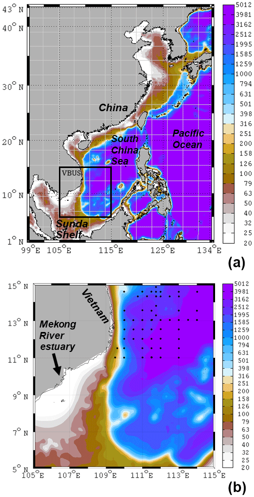
Figure 1(a) Model domain and the bathymetry (unit: m) for the Taiwan Strait Nowcast/Forecast system and carbon, silicon, nitrogen ecosystem (TFOR-CoSINE) model. Model grid nodes are shown every 25 points. The study area VBUS is boxed. (b) Zoom-in area of VBUS. Black diamonds are the observation stations (see text).
In the VBUS, the upwelling intensity is governed by the strength of the alongshore monsoon wind, as in other coastal upwelling systems such as the coastal upwelling systems of California and Mid-Atlantic Bight (Gruber et al., 2011). The VBUS upwelling strength is intense and can result in surface cooling of 3–5 ∘C and an associated cold filament length of ∼500 km (Kuo et al., 2004). The VBUS is modulated by different climatic variations, such as the El Niño–Southern Oscillation (Dippner et al., 2007; Hein et al., 2013; Xie et al., 2003), the Indian Ocean dipole (Liu et al., 2012; Xie et al., 2009), and the Madden–Julian oscillation (Isoguchi and Kawamura, 2006; Liu et al., 2012).
Previous studies suggested that both the wind-induced upwelling and the local circulation could influence the nutrient balance and ecosystem in the VBUS. The El Niño variability is an important controlling factor of the VBUS by modulating the summer monsoon (Chai et al., 2009; Kuo et al., 2004). During post-El Niño summer, the weakened southwesterly wind leads to weak upwelling and reduced upward nutrient flux (Xie et al., 2003). In addition, Hein et al. (2013) proposed instead that productivity was controlled by lateral transport of nitrate in the VBUS. Liu et al. (2002) also highlighted the role of coastal jet located to the south of the Vietnamese coast. They mentioned that jet-induced upwelling was responsible for the nutrient influx. Xie et al. (2003) mentioned the role of the offshore jet and resultant quasi-stationary eddy (i.e., the “recirculation” hereafter) in transporting the highly productive water. However, the contribution from recirculation has not been directly quantified and compared with that directly from the upwelling, which motivates us to revisit the VBUS ecosystem and its connection with circulation.
Early hydrodynamic observations revealed a northeastward coastal current over the southern shelf of Vietnam (Wyrtki, 1961). The current separates from the coast and flows offshore at about 11∘ N (Xu et al., 1982). Xie et al. (2003) ascribed the jet separation to the strong wind jet off Vietnam due to the orographic steering of the north–south running mountains. Using an idealized reduced gravity model, Wang et al. (2006) highlighted vorticity input by wind-stress curl and vorticity advection by the basin circulation. Gan and Qu (2008) found that the separation was associated with an adverse pressure gradient induced by the topographic effects.
The separated jet produces cooling and results in biannual sea surface temperature (SST) variation in the SCS (Xie et al., 2003). The offshore jet also appears to advect water with high chlorophyll to the interior of the central SCS (Chen et al., 2014; Loisel et al., 2017; Tang et al., 2004). While the importance of the local current system to the VBUS biogeochemical system has been noted in some previous studies (Dippner et al., 2007; Kuo et al., 2004; Liu et al., 2012; Xie et al., 2003), the detailed processes are unclear. To what extent is the ecosystem in the VBUS modulated by local circulation? Does the circulation show any distinction in the high/low production cases? How does the recirculation modulate productivity? How much does the local circulation contribute to production? Studying biological production and its coupling with physical processes in the VBUS will help to answer these questions and further improve the understanding of boundary upwelling systems. Such a study will also shed light on the ecosystem dynamics in the SCS as an oligotrophic marginal sea. Here, we analyze the complex dynamics of the VBUS using a physical–biological coupled numerical model system, as well as remote sensing data and in situ observations.
This paper is organized as follows. In Sect. 2, the model configuration, numerical experiments, observed data, and statistical method used in this study are described. In Sect. 3, we analyze the remote sensing data and validate the model. Model results from both the standard run and the sensitivity experiment are presented. In Sect. 4, the dynamical processes are analyzed. Conclusions are given in Sect. 5.
2.1 Data
The surface wind vectors were from the Cross-Calibrated Multi-Platform (CCMP) gridded data. This is a 25-year, 6-hourly, resolution product fused from several microwave radiometers and scatterometers using a variational analysis method (Atlas et al., 2011). Monthly Moderate Resolution Imaging Spectroradiometer (MODIS) Aqua level 3 chlorophyll (4 km resolution) was obtained from the NASA Distributed Active Archive Center. The estimated monthly vertical-integrated net primary production (NPP) was derived from MODIS chlorophyll data via the standard chlorophyll-based Vertically Generalized Production Model (VGPM) algorithm (Behrenfeld and Falkowski, 1997). The VGPM NPP product had a resolution of 1∕10∘, covering the period from 2004 to the present. Gridded monthly mean absolute dynamic topography (ADT) with respect to the geoid at 1∕4∘ resolution was acquired. The 1∕4∘ optimum interpolation sea surface temperature (OISST, also known as Reynolds 0.25v2) was constructed by combining the Advanced Very High Resolution Radiometer satellite and other observation data (Banzon et al., 2016). Atmospheric forcing including downward shortwave radiation, downward longwave radiation, air temperature, air pressure, precipitation rate, and relative humidity were acquired from the National Centers for Environmental Prediction reanalysis (Kalnay et al., 1996). The river runoff data (see Sect. 2.3 below) were adopted from Dai et al. (2009), which contains observation-based monthly freshwater runoff of major rivers of the world. The climatology of temperature, salinity, nutrients, and dissolved organic matter was adopted from the World Ocean Atlas (WOA, 2013 version). In situ observed nitrate and chlorophyll profiles from the western SCS stations (Fig. 1b) were used, as detailed in Jiao et al. (2014).
2.2 Methods
2.2.1 Upwelling intensity (UI) and kinetic energy (KE)
We use the upwelling intensity (UI) or the “Bakun index” (Bakun, 1973) as a proxy to measure the strength of upwelling (Chen et al., 2012; Gruber et al., 2011), following the classical paper of Ekman (1905):
Here, τy is the alongshore component of wind stress, f is the Coriolis parameter, ρ0 is seawater density (constant, 1025 kg m−3), ρa is the air density (constant, 1.2 kg m−3), CD is the drag coefficient (constant, ), and Uy is the alongshore wind speed. The CCMP data with full temporal and spatial coverage close to the coastline are used for the wind speed.
The kinetic energy (KE) of the near-surface current is used as an indicator of the circulation intensity. The near-surface current is calculated from ADT using the geostrophic balance. The KE then equals
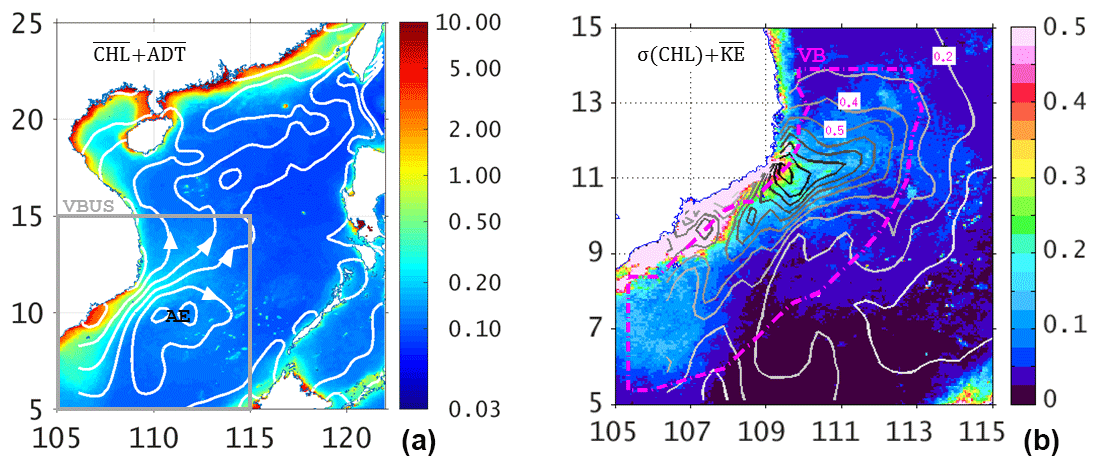
Figure 2(a) Summertime (MJJAS) average of surface chlorophyll concentration (color shading, unit: mg m−3) from MODIS; overlapped white contours are the mean ADT, with the arrows showing the directions of surface currents. The gray box is the region of interest (VBUS), while AE shows the center of the anticyclone. (b) Standard deviation of surface chlorophyll (color shading, unit: mg m−3) overlapped with the contours of surface KE with an interval of 0.1 from 0.1 to 1.0 (unit: m2 s−2). The magenta dot–dash contour delimits the ocean region over which chlorophyll and KE are averaged (see text).
2.2.2 Multivariable linear regression
Monthly NPP from VGPM (see Sect. 2.1) was used to estimate biological productivity. A multivariable linear regression analysis was conducted to examine the statistical relations among NPP, UI, and KE:
where b1, b2, and b3 are the estimated parameters of the regression. Data in the summer months (MJJAS) were used since the monsoon wind during this period is upwelling favorable. The focus region of this study is not confined to the “actual” upwelling strip of ∼40 km width as indicated by the first baroclinic Rossby radius of deformation (Dippner et al., 2007; Voss et al., 2006) but extended to a broader offshore region of ∼3∘ width. Therefore, we averaged NPP and KE over the ocean region enclosed by the magenta contour off the coast of Vietnam (Fig. 2b). Only the summertime data in the overlapping period from 2004 to 2012 were analyzed. Contributions from SST, day length, and the photosynthetically active radiation were implicitly considered in the VGPM (Behrenfeld and Falkowski, 1997).
2.3 Model description
We use a three-dimensional general circulation model based on the Regional Ocean Model System (ROMS). ROMS is a free-surface and hydrostatic ocean model. It solves the Reynolds-averaged Navier–Stokes equations on terrain-following coordinates (Shchepetkin and McWilliams, 2005). The model is used in the operational Taiwan Strait Nowcast/Forecast system (TFOR), which successfully provides multi-purpose ocean forecasts (Jiang et al., 2011; Liao et al., 2013; Lin et al., 2016; Lu et al., 2017, 2015; Wang et al., 2013). In this study, the model grid is modified to cover the whole SCS domain and part of the northwestern Pacific with a grid resolution of 1∕10∘ (Fig. 1a). The number of grid nodes in x and y directions is 382 and 500, respectively. In the vertical, 25σ levels is used with a grid size of ∼2 m on average near the surface to resolve the surface boundary layer. Following the bulk formulation scheme (Liu et al., 1979), daily atmospheric fluxes (detailed in Sect. 2.1) are applied at the surface. The wind vectors are from the CCMP wind. The vertical turbulent mixing uses a K-profile parameterization (KPP) scheme (Large et al., 1994) which was successfully applied in a one-dimensional vertical mixing model in the SCS (Lu et al., 2017). The KPP scheme estimates eddy viscosity within the boundary layer as the production of the boundary layer depth, a turbulent velocity scale, and a dimensionless third-order polynomial shape function. Beyond the surface boundary layer, the KPP scheme includes vertical mixing collectively contributed by shear mixing, double diffusive process, and internal waves. Biharmonic horizontal mixing scheme (Griffies and Hallberg, 2000) with a reference viscosity of 2.7×10¹⁰ m4 s−1 is applied, following the value of Bryan et al. (2007) used in a circulation model with the same horizontal resolution. Climatological river discharge from the Mekong River and other major rivers is included as point sources.
The biogeochemical module is the carbon, silicon, nitrogen ecosystem (CoSINE) model (Xiu and Chai, 2014), which consists of 31 state variables, including four nutrients – nitrate (NO3), ammonium (NH4), silicate, and phosphate, three phytoplankton functional groups (representing picoplankton, diatoms, and coccolithophorids), two zooplankton classes (i.e., microzooplankton and mesozooplankton), four detritus pools (particulate organic nitrogen/carbon, particulate inorganic carbon, and biogenic silica), four kinds of dissolved organic matter (labile and semi-labile pools for both carbon and nitrate), and bacteria. Other planktonic groups can be important in the ecosystem of SCS in some condition (Bombar et al., 2011; Doan-Nhu et al., 2010; Loick-Wilde et al., 2017). Surely, adding more planktonic groups would better depict the complex relationship in the ecosystem. However, considering the functional groups chosen here were dominating species widely observed in the SCS (e.g., Ning et al., 2004), adding more planktonic species is unlikely to radically change the spatiotemporal variation of the modeled ecosystem. To keep the ecosystem model simple and computationally affordable, these groups are not considered in the CoSINE model. The CoSINE model was well applied in various studies of the SCS. Liu and Chai (2009) investigated the seasonal and interannual variability of the primary productivity of the SCS at a basin scale. The modeled structure (e.g., phytoplankton community) and function (e.g., biological pump) of the ecosystem appeared to respond to both climatic variations (Ma et al., 2013, 2014) and mesoscale eddies (Guo et al., 2015), both well captured by CoSINE. By taking a SCS average, the modeled NPP time series showed a strong correlation (R=0.84) when compared with satellite-derived production (Ma et al., 2014). Details of the CoSINE results in SCS can also be found in Lu et al. (2018).
The physical model was initialized from a resting state with temperature and salinity specified using the WOA climatology. The initial distribution of the nutrients and dissolved organic matter was also interpolated from the WOA climatological data. Our previous studies related with ecosystem modeling in the Chinese seas (Lu et al., 2015; Wang et al., 2016, 2013) suggested that the ecosystem module was more sensitive to the initial value of nutrients and dissolved organic matter. For other variables (i.e., detritus and plankton), the model converged to similar states even when these variables were initialized differently. Hence, for these ecosystem variables, small values were assigned as in Table S1 in the Supplement. After spinning up for 13 years with climatological forcing, the model was restarted with the ecosystem module driven by interannually varying CCMP wind and atmospheric surface forcing from 2002 to 2011. The model output from 2005 to 2011 is analyzed.
2.4 Sensitivity experiment
To quantify the contribution to the ecosystem from the recirculation, we seek to control the formation of the recirculation while maintaining the larger basin-scale circulation. For the Vietnam boundary upwelling system, since nonlinear advection is important to the separation of the coastal jet and thus the formation of the anticyclone (Gan and Qu, 2008; Wang et al., 2006), which is familiar in the Gulf Stream separation problem (Haidvogel et al., 1992; Marshall and Tansley, 2001), an experiment without the nonlinear advection terms in the momentum equations was conducted (following, e.g., Gruber et al., 2011). It should be noted that the advection terms in the tracer equations are retained for transport of active and passive tracers (i.e., ecosystem variables). Hereafter, this experiment will be referred to as the NO_ADV run.
In this section, we first analyze the satellite-based observational data, focusing on the spatiotemporal covariance of wind, circulation, and biological production. After accessing the model performance against observation, we then describe and discuss the model results.
3.1 Spatiotemporal analysis of observation data
Figure 2 shows the mean (Fig. 2a) and standard deviation (Fig. 2b) of surface chlorophyll overlaid with contours of mean ADT and KE, respectively. In summer, the surface chlorophyll has a low concentration of <0.1 mg m−3 in the central SCS basin. By contrast, the chlorophyll is more than 5-fold (>0.5 mg m−3) along the southern Vietnamese coast. The high chlorophyll water appears to extend offshore following the coastal jet to the interior SCS. The jet overshoots after separating from the coast and bifurcates into a northeastward current and a quasi-stationary anticyclonic eddy (Fig. 2a). Centered at ∼11∘ N near the tip of the Vietnamese coast, high KE (>1.0 m2 s−2) appears near the coast. The high variability of chlorophyll coincides with KE into the interior SCS, implying the contribution from the jet (Fig. 2b).
The box-averaged (magenta box in Fig. 2b) time series of monthly UI, KE, and NPP are shown in Fig. 3a–c; they show seasonal and interannual variations. KE and NPP both present biannually signals in most years, i.e., peaks in summer and winter, as well as complex non-seasonal signals. Unsurprisingly, UI dominates about half (R2=0.4548 for UI solely, p<0.01) of the total variability in NPP, which is consistent with studies in other wind-driven upwelling systems (Gruber et al., 2011), and with the previous studies of the VBUS (Bombar et al., 2010; Voss et al., 2006). The correlation between KE and NPP is even higher (R2=0.4930, p<0.01). Moreover, although KE could be dependent on the wind, the R2 between KE and UI is 0.3240, suggesting that a large part (∼68 %) of the variation in KE is unexplained by the uniform alongshore wind. There are clear positive contributions to the biological production from both UI and KE. When KE and UI are considered concurrently, an additional ∼15 % of the variability in NPP is explained (R2=0.6046, p<0.01).
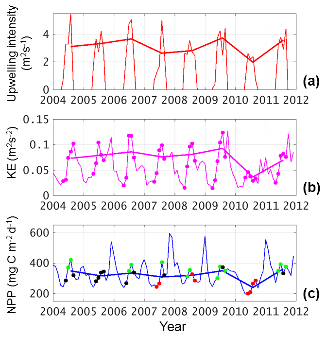
Figure 3Time series of (a) UI in m2 s−1, (b) KE in m2 s−2, and (c) NPP in mg C m−2 day−1 of monthly data (thin lines) and summer mean (thick lines). In panel (a), only the positive (upwelling-favorable) values are shown. In panel (b), months with positive UI are marked with dots. In panel (c), green, black, and red dots indicate high NPP anomaly (HNA), normal, and low NPP anomaly (LNA) scenarios.
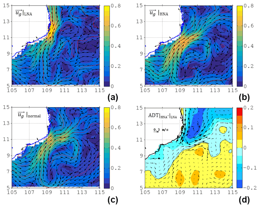
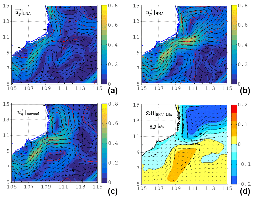
Figure 4The surface current velocity (color shading, unit: m s−1), direction (vectors), and respective ADT (red contours, unit: m) in (a) LNA, (b) HNA, and (c) normal months (i.e., neither LNA nor HNA) scenarios (see text for criteria). (d) The differences of ADT and current between HNA and LNA.
To further illustrate the modulation in the ecosystem by circulation, the flow patterns in high NPP anomaly (HNA) and low NPP anomaly (LNA) were composited according to the de-seasonalized NPP anomaly (Fig. 3c). The seasonal signal was firstly removed from the summertime NPP, yielding the de-seasonalized NPP anomaly. The thresholds for HNA and LNA are defined as (above) 75 % and (below) 25 % percentile of the NPP anomaly, respectively. Different thresholds (60 % and 70 %) were also tested and very similar results can be seen. The velocity and direction for LNA, HNA, and the normal state (i.e., neither LNA nor HNA) are respectively depicted in Fig. 4a–c, as well as the ADT difference between HNA and LNA (Fig. 4d). A Student's t test suggests that the three circulation patterns are significantly (p<0.01) different. In contrast to the familiar separation and offshore jet pattern (Figs. 2a and 4c), the LNA circulation tends to flow along the coast without separation (Fig. 4a). On the other hand, the HNA circulation (Fig. 4b) shows a clear separated jet and anticyclonic recirculating pattern south of the jet near 8.5∘ N, similar to the pattern seen during normal years (Fig. 4c); the flow speed is ∼20 % stronger than that of the normal state. Near the separation point, the HNA jet is more dissipated and slightly weakened compared with the LNA coastal jet. The KE averaged within the magenta box (Fig. 2b) during the HNA state is 0.0827 m2 s−2, which is ∼65 % larger than that during the LNA state (0.0502 m2 s−2). The difference in flow patterns is consistent with a dipolar ADT difference, by which a westward (inverse to the jet) pressure gradient force anomaly is imparted to the flow (Fig. 4d), which is responsible for the jet separation process (Batchelor, 1967; Gan and Qu, 2008). In order to examine the recirculation's role in the ecosystem, we now use the model to address the physical–biogeochemical coupling.
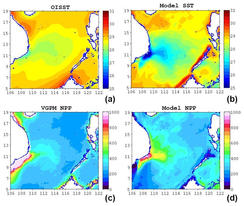
Figure 5(a) OISST, (b) model SST (unit: ∘C), (c) VGPM NPP, and (d) modeled NPP (unit: mg C m−2 day−1) in multi-year August average.
3.2 Model validation
In Fig. 5, simulated SST and NPP are compared with observations. The model reproduces reasonably well the observed patterns of SST and NPP. In particular, the model captures the cross-shore SST gradient. The cold filament that overshoots from the coast to the interior of SCS is also clearly reproduced by the model. However, the modeled SST shows a systematic cold bias of ∼ 1 ∘C, and the modeled NPP does not simulate well the extremely high values (>1000 mg C m−2 day−1) along the Vietnamese coast. This may in part be attributed to overestimation of retrieved NPP near the coast (Loisel et al., 2017). Off the coast, the model simulates well the cross-shore gradient of productivity. The gradient is generally high in areas influenced by the jet. In the coupled model, while it is true that SST affects NPP through, for example, changes in the vertical stratification of the water column, both SST and NPP strongly depend on circulation (e.g., upwelling and/or downwelling), and in our case on the flow separation and KE also. In turn, the circulation is dominated by changes in the upper-layer depth (as diagnosed through the SSH) and the horizontal gradients of SSH, and is much less dependent on the gradients of SST. Thus, the covariation between the SST and ecosystem is largely controlled by the circulation. The dominant ecosystem response is the separation and non-separation contrast, which is captured well by the model (comparing Figs. 4 and 8).
Time series of modeled SST, surface KE, and NPP, averaged over the magenta contour region (Fig. 2b), are compared with observations in Fig. 6. Due in part to the realistic surface forcing and high resolution used, our model can reproduce the physical and biological variables in the VBUS. The seasonal cycles in all three quantities agree reasonably well with the observations. At interannual timescales, during the 2010 El Niño event, for example, the monsoon was weaker (Fig. 3a), SST was warmer, and the KE was reduced. These features are simulated well, although the production drawdown is slightly weaker than the observation and the simulated SST underestimates amplitude of the observed SST annual cycle by ∼1.0 ∘C. For the surface current and productivity, our model shows excessive KE and insufficient production during winter, but the model–observation discrepancy is less notable in other seasons. The overestimated KE is partially contributed by the Ekman component in the modeled surface current. Nevertheless, we can conclude that our model reasonably reproduced the temporal variability in the VBUS.

Figure 6Thick lines: modeled (a) SST in ∘C, (b) KE in m2 s−2, and (c) NPP in mg C m−2 day−1 averaged over the box region (see Fig. 2b), with respective observation data (thin dashed lines). Correlation coefficients are also shown in each plot. In panel (c), green, black, and red dots indicate HNA, normal, and LNA scenarios (see text for definition).
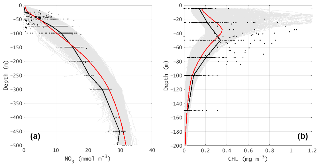
Figure 7The vertical profiles of (a) nitrate concentration (unit: mmol m−3) and (b) chlorophyll concentration (unit: mg m−3). In both plots, the black dots are the observation values (see Fig. 1b for stations). The gray area shows the envelope for all model stations in the same area and month, while the red lines are the area-mean profiles.
In addition, vertical profiles of the simulated NO3 and chlorophyll, as two fundamental components of the marine ecosystem, are compared with observations (Fig. 7). The modeled NO3 generally reflects the oligotrophic condition near the surface and the nutricline approximately at 50 m. Below the nutricline, the NO3 profile shows moderate vertical gradient to the deep. The simulated NO3 profile matches the observations remarkably well. For the chlorophyll, our model well simulates the concentration, not only at the surface but also in the deep layer. A subsurface chlorophyll maximum appears at ∼35 m, which is somewhat shallower than that in the observation (50 m). Except for model uncertainty, this discrepancy may also be related to the undersampling in observed profiles (no water samples between 25 and 50 m depth). When chlorophyll is considered as a proxy of NPP, vertically integrated chlorophyll is more relevant. The vertical-averaged (5 to 150 m) chlorophyll concentrations in the model and observation are 0.1595 and 0.1668 mg m−3, respectively, which have a marginal difference (<5 %). Both the modeled and observed chlorophyll concentrations have a large range from 0 to >1.0 mg m−3 in the subsurface chlorophyll maxima. This reflects the large spatial variability in chlorophyll.
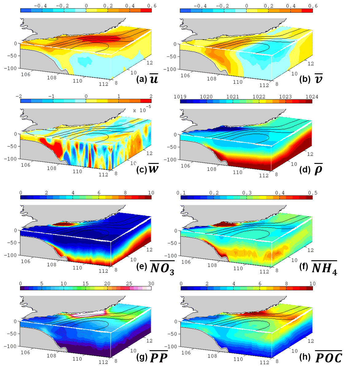
Figure 9Three-dimensional distribution (standard run) of the summer mean (a) zonal velocity in m s−1, (b) meridional velocity in m s−1, (c) vertical velocity in m s−1, (d) potential density in kg m−3, (e) nitrate in mmol m−3, (f) ammonium in mmol m−3, (g) primary production in mg C m−3 day−1, and (h) particulate organic carbon in mmol C m−3. Overlapped contours are the mean sea level (every 0.1 m).
Following the analysis in Sect. 3.1, the multi-variable regression analysis on the model output was also conducted. The modeled NPP presents a phase lag with respect to the UI and KE variation. When NPP is lagged for 1 month, the correlation is 0.752 with a p value of 0.0214, suggesting a significant regulation of the physical forcing to the productivity. Additionally, the composites of the HNA, LNA, and normal scenarios (Fig. 6c) based on model output show contrasts among scenarios comparable to those in the observed cases in Fig. 4, further suggesting the reasonability of the model simulation (Fig. 8).
In summary, one could find that our model performs reasonably in reproducing the key spatiotemporal features in the hydrodynamics and ecosystem of VBUS. Inevitably, some discrepancies exist, which are less evident in the summer months. Nevertheless, considering the focus is to investigate the positive correlation between the productivity and the circulation, which was captured by the model (Fig. 8), these shortcomings could be accepted.
3.3 Analysis of model results
Modeled circulation and potential density from the multi-summer average are presented in Fig. 9a–d, with sea surface height overlaid. In the upwelling region, the doming of isopycnals (Fig. S2) is discernable as in the classical coastal upwelling models (O'Brien and Hurlburt, 1972). Consistent with previous studies, the coastal current flows northward along the shelf (Hein et al., 2013). The current also disperses freshwater from the Mekong River, while the water seldom spreads away from the coast. The coastal current veers at ∼11∘ N, directs offshore, and then separates, forming the quasi-stationary anticyclone centered at ∼ 9∘ N, 110∘ E. Near the core of the anticyclone, vigorous vertical motion near the surface can be found, implying submesoscale processes in play. Near 108∘ E, intensive onshore flow ascends on the slope. The high-density bottom water outcrops at 107∘ E, rejoining the coastal water and directing north, thus forming a circuit.
The biogeochemical variables reveal that the ecosystem is largely controlled by the circulation (Figs. 9e–h, S2). Lateral nutrient gradient appears at the periphery of the anticyclone, which is characterized with depressed nitrate isosurface in the core and domed isosurface due to the upwelling and river injection near the coast (Fig. 9e). Stimulated by the river-injected and locally upwelled nutrients near the coast, primary production (PP) shows a surface maximum of >30 mg C m−3 day−1 (Fig. 9g). The water with high production is then advected offshore by the jet (Fig. 9h), leading to an offshore bloom patch in a curved shape which is familiar along the Vietnamese coast (e.g., Fig. 5c). The jet also conveys the water with high particulate organic carbon offshore. The distribution of particulate organic carbon is somewhat deeper and more spread than that of high PP water, suggesting the vertical sinking and lateral transport processes (Nagai et al., 2015). Remineralization of organic carbon results in a subsurface ammonium maximum at ∼50 m (Fig. 9f) consistent with other studies in SCS (Li et al., 2015). Part of the ammonium could then fuel nitrification and production, while the rest rejoins the circulation with the upwelling water in the bottom Ekman layer. In summary, the model output clearly reveals circuiting circulation and a cycled ecosystem, which will be further discussed in Sect. 4.
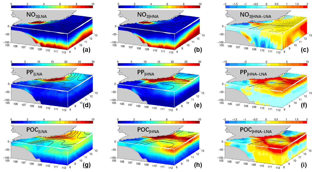
Figure 10Modeled NO3 (a–c, in mmol m−3), PP (d–f, mg C m−3 day−1), and particulate organic carbon (g–i, mmol C m−3) distribution in LNA (a, d, g), HNA (b, e, h), and the difference between two scenarios (c, f, i). See text for the definition of LNA and HNA.
4.1 Biogeochemical cycle in the VBUS
In the summer VBUS system, it is generally agreed that the wind's predominant role is controlling the variability in the production of VBUS, especially on the interannual scale (Dippner et al., 2013). This is also the case in our analysis, where UI contributes ∼45 % of the total variability in production. In addition, via analysis of satellite data and model output, consistent and robust positive contribution from the local circulation to the biological production was also revealed. The contribution of the circulation is distinct from the major coastal upwelling systems, where the offshore transport by the mean current appears to suppress the production by reducing the nearshore nutrient inventory (Gruber et al., 2011; Nagai et al., 2015). The separated current system was considered to transport high-chlorophyll water offshore (Xie et al., 2003). In the offshore region, the production appeared to be elevated (Bombar et al., 2010). However, the fate of the offshore nutrients was rarely investigated in the literature.
Table 1Summery of the ecosystems in three model scenarios.
∗ See Fig. 11a for the location.
Comparing the ecosystems in LNA and HNA (Fig. 10), the following stages of the cycle can be deduced: (1) the upwelled and riverine input nutrients (majorly inorganic) stimulate high production near the Vietnamese coast (Dippner et al., 2007); (2) the produced organic matter is transported offshore by the jet; the water has high chlorophyll (e.g., Fig. 2a) and high organic matter (Fig. 9h) in the euphotic zone; (3) a significant portion of the nutrients (majorly in organic form) is transported back to the south of VBUS by the westward recirculation. The quasi-stationary rotating anticyclone impedes further offshore leakage of the nutrients (Fig. 10i). (4) The trapped organic matter is remineralized, forming the subsurface maxima of ammonium (Fig. 9f, which supports regeneration production with an f ratio of ∼60 %, Table 1) and replenishing the nitrate by nitrification. The offshore remineralization can be supported by the high oxygen consumption found off Vietnamese coasts (Jiao et al., 2014). Afterward, the nutrients are upwelled by bottom Ekman pumping (see high amount of nutrients in the bottom boundary layer in Fig. 9e) and wind-induced upwelling, and finally rejoin in the local biogeochemical cycle. The recirculation may determine the available nutrient inventory, therefore playing a significant role in controlling the productivity, which will be further supported by the experiment in the following section.

Figure 11(a–c) Modeled 0–100 m integrated nitrate fluxes (unit: mmol s−1) in horizontal plane. Color shading indicates the magnitude, while vectors denote the direction. (d–f) Vertical flux across 100 m level for normal year (a, d, years other than 2010), NO_ADV case (b, e), and post-El Niño (c, f, in 2010). Overlapped contours are the 50 and 75 m isobaths. In panel (a), the magenta line is the 109∘ E section (Table 1).
4.2 Dynamic analysis
By controlling the available nutrients, the recirculation modulates the productivity in the VBUS. The influence of the recirculation is further elucidated below. Table 1 summarizes the difference of the ecosystems in the standard run and NO_ADV experiment. The NO_ADV experiment can be regarded as an extreme case where the circulation shows very weak tendency of separation without the recirculation (also see Fig. S1), which is representative of the LNA scenario. In terms of force balance, the recirculation is maintained by the balance between the inertial force and the Coriolis force. Without the nonlinear term, this balance could not exist. The horizontal and vertical fluxes of nitrate in three scenarios are also depicted in Fig. 11.
In the VBUS, similar to other coastal upwelling systems (Steemann-Nielsen and Jensen, 1957), the availability of nutrients principally controls the productivity. Considering a quasi-steady state of nutrients in a coastal region, river-injected and upward inputted nutrients should be counter-balanced by vertical export production and lateral exchanges. The lateral exchanges include both advection and diffusion, while it was pointed out that horizontal mixing is 1 or 2 orders of magnitude lower than that of horizontal advection (Lu et al., 2015). Hence, as a sink term, the lateral exchanges are determined mostly by the advective fluxes normal to the boundary of the predefined box. The diagnostic also suggests a dominance role of advection process in the vertical overmixing. Given the fact the standard run and NO_ADV experiment have the same riverine input and similar export flux, one could infer that the difference between two model cases is largely due to the different lateral transports and upwelled fluxes of nutrients.
In the LNA (Figs. 4a and 8a), and also in the NO_ADV experiment (Fig. S1), the circulation pattern switches to the along-isobath pattern, which modifies the local biogeochemical cycle. More nutrients are transported northward and offshore out of VBUS and never come back, leading to a reduction of nutrients (Fig. 11). This effect can be demonstrated by cross-section nutrient flux across the 109∘ E section. The more nutrient leakage, the less westward nutrient flux across this section. In the NO_ADV run, the westward flux of nitrate is significantly reduced by 36.2 % (Table 1). The reduction of nutrients is accompanied by suppressed the upward nutrient flux (−46.5 %) near the shelf edge (∼100 m). As a consequence of more leakage and less upwelling influx, the nitrate reservoir and new production are significantly reduced by 20.7 % and 21.9 %, significantly inhibiting the primary production process (15.7 %, Table 1). Other ecosystem constituents decrease to a limit degree, such as −2.6 % for ammonium and −3.0 % for dissolved organic carbon (DOC). This interpretation is further supported by the post-El Niño scenario. In 2010, more significant suppression occurs in the vertical nutrient flux (−99.6 %), while the horizontal fluxes also respond to decrease. Due to the drawdown in the wind-induced upwelling and recirculation (Table 1), the production is extremely low in summer 2010 (Fig. 3c).
The larger the KE, the more intensive the separation (see Appendix B for additional discussion about this point). This separation was similar to the Gulf Stream detachment problem in many aspects. In particular, various factors could affect the intensity and position of the separation (Chassignet and Marshall, 2008). Generally, the mechanism of the current separation was considered to be ascribed to the wind stress curl (Xie et al., 2003). We also found that the current separation was very sensitive to the wind stress curl (not shown in figures). Hence, one may argue that this covariability is controlled by the variation of wind forcing. However, as mentioned in Sect. 3.1, a large part (∼68 %) of the variation in KE is unexplained by the large-scale wind. In addition, our sensitivity experiments without the nonlinear advection of momentum showed very weak separation, in agreement with that of Wang et al. (2006). This implies wind forcing is not the only factor in controlling the current system, while the intrinsic dynamics are also important. The accelerated coastal current is also associated with intensified cross-isobath transport by bottom Ekman effect (Gan et al., 2009) or dynamic upwelling (Yoshida and Mao, 1957) due to the rotational current (Dippner et al., 2007). Hence, low KE reduces the recirculation of nutrients. Combining all the effects, the intensified current is a condition favorable for the nutrient inventory and hence the productivity. To a larger scale, the recirculation current couples coastal upwelling and the offshore region in the major coastal upwelling systems, e.g., in the Canary basin (Pelegrí et al., 2005). In this study, this effect was also found to be important, which may contribute up to 15 % of the productivity variability.
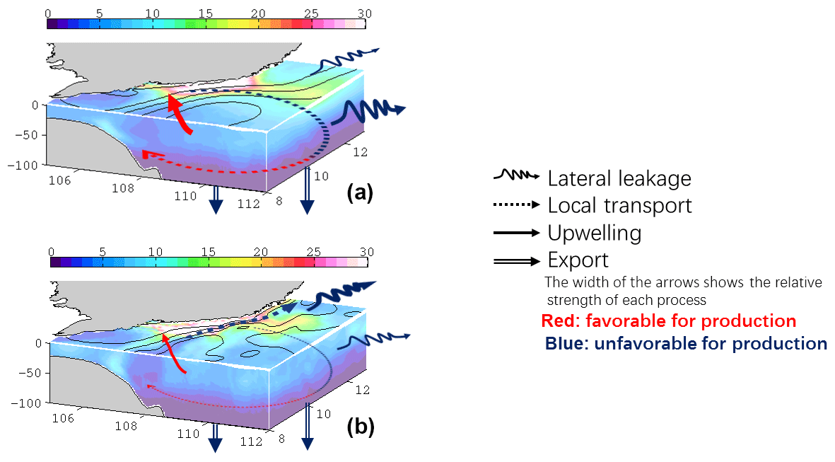
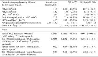
Figure 12Schematic diagram summarizing the dynamics in different scenarios of distinct circulation pattern in the VBUS, overlapped with the three-dimensional distribution of PP (unit: mg C m−3 day−1). (a) Normal state: the separated jet transports the upwelled nutrients and produced organic matter offshore. While a substantial portion of the offshore transported organic matter leaks into the interior of SCS and never comes back, the recirculation and quasi-stationary anticyclonic eddy trap the organic matter locally and hinder further leakage of available nutrients in the VBUS. The locally recirculated nutrients are then upwelled in the bottom Ekman layer, rejoining the production process over the shelf. (b) Non-separation state: during the non-separated circulation, the along-isobath circulation transports the organic matter northward. The leakage of organic matter reduces the nutrient inventory in the VBUS. The loss of nutrients diminishes the nutrient inventory available for remineralization and upwelling, further inducing a reduction in the production process.
Via analyzing the summertime remote sensing data in the VBUS, a tight spatiotemporal covariation between the ecosystem and near-surface circulation was revealed. The water with high kinetic energy appeared to coincide with high chlorophyll variability. Statistical analysis suggested that the high level of productivity was associated with the high level of circulation intensity, which accounted for ∼ 15 % of the variability in productivity. Elevated kinetic energy and intensified circulation were related to the separation of the upwelling current system. Especially, in the low-productivity scenarios, the circulation pattern shifted from the intensive separation pattern to a moderate alongshore non-separated pattern.
A physical–biological coupled model was applied to investigate the positive contribution from the circulation intensity to the productivity. A numerical experiment was also designed to reproduce the weak-separated circulation pattern without the recirculation. Inspection into the model results highlighted the recirculation's role in the local biogeochemical cycle. As presented in the schematic diagram in Fig. 12, the separated circulation and resultant recirculation were favorable for the nutrient inventory. During non-separation scenarios, the nutrients transported northward by the alongshore current would never come back, leading to a nutrient leakage. The nutrient leakage further induced the feedback summarized in Fig. 12b, which could reduce the nitrate inventory by ∼21 % and the NPP by ∼16 % in the experiment representative for very weak separation. The weakened coastal current was also associated with reduced dynamic upwelling, hence further reducing the vertical flux of nutrients. This resulted in the positive contribution to the productivity.
This finding provides new insight into the complex physical–biological coupling in the Vietnam coastal upwelling system. Moreover, this understanding could help to predict the future reaction of productivity in the SCS. As revealed by Yang and Wu (2012), the summertime near-surface circulation of SCS had experienced a long-term trend of being more energetic, characterized with intensified separation and recirculation in the VBUS (see their Fig. 9). Whether this long-term trend of circulation will also induce a potential trend in the ecosystem in response to future climate changes is a topic of common interest, which merits further investigation.
The CCMP gridded Ocean Surface Wind Vector L3.0 first-look analyses (version 1) data were accessed 12 March 2015 at https://doi.org/10.5067/CCF30-01XXX (NASA/GSFC/NOAA, 2009). The MODIS Aqua level 3 chlorophyll data were accessed at http://oceancolor.gsfc.nasa.gov (last access: 16 May 2014). The VGPM NPP data were available at http://www.science.oregonstate.edu/ocean.productivity/index.php (created by Oregon State University, last access: 18 October 2018). Gridded monthly mean ADT, available at http://www.aviso.altimetry.fr/en/data/products/sea-surface-height-products/global/ (last access: 12 March 2016), was produced by Ssalto/Duacs (http://www.aviso.oceanobs.com/duacs/, last access: 12 March 2016), and was distributed by Aviso with support from the Centre National d'Études Spatiales (CNES). The OISST data were obtained from the National Climatic Data Center of NOAA (https://www.ncdc.noaa.gov/oisst/data-access, last access: 18 October 2018). Atmospheric forcing data were acquired from the National Centers for Environmental Prediction reanalysis data (http://www.esrl.noaa.gov/psd/data/gridded/data.ncep.reanalysis.html, last access: 18 October 2018) distributed by the NOAA/OAR/ESRL PSD, Boulder, CO, USA (http://www.esrl.noaa.gov/psd/, last access: 18 October 2018). The WOA data distributed by National Climatic Data Center of NOAA were available at https://www.nodc.noaa.gov/OC5/woa13/ (last access: 18 October 2018). The river runoff data were available at http://www.cgd.ucar.edu/cas/catalog/surface/dai-runoff/ (last access: 18 October 2018), which was created by the University Corporation for Atmospheric Research.
| Abbreviation | Definition |
| SCS | South China Sea |
| VBUS | Vietnam boundary upwelling system |
| CCMP | Cross-calibrated multi-platform data |
| MODIS | Moderate Resolution Imaging Spectrora- diometer |
| VGPM | Chlorophyll-based vertically generalized production model |
| ADT | Absolute dynamic topography |
| OISST | Optimum interpolation sea surface tem- perature |
| HNA/LNA | High/low NPP anomaly scenario |
| NPP | Vertical-integrated net primary produc- tion |
| PP | Primary production (as a function of depth) |
| KE | Kinetic energy |
| TFOR | Taiwan Strait Nowcast/Forecast system |
| CoSINE | Carbon, silicon, nitrogen ecosystem model |
| NO_ADV | Model experiment with no advection term in momentum equations |
| UI | Upwelling intensity |
Qualitatively, both the analyses based on remote sensing data and model results suggest the separation flow is linked with stronger KE (∼65 % larger in the HNA case than in the LNA case; Sect. 3.1). Moreover, a separation index (SI) is defined to quantitatively explain the relation between the flow separation and intensified circulation. The SI can be written as
where u and v are the two surface velocity components, and φ is the angle between the topography gradient and the positive x axis. This SI is essentially the area-averaged cross-isobath velocity normalized by the magnitude of the velocity, which is used to quantify flow separation here.
Figure B1 shows the spatial distribution of SI in August 2010. The positive values indicate the flow is downslope, while negatives suggest ascent. Large SI can be observed near the separation point (∼ 11.5∘ N). Taking the spatial average over the box region in Fig. B1, a generally good positive correlation (R=0.7175, p<0.01) between log(KE) and SI is found (see Fig. B2). The log(KE) and SI presents a logistic-type relationship, where SI asymptotically approaches a maximum value of ∼0.35. This suggests that the strong flow separation and elevated KE are tightly linked. Further, from the scatter plot of KE vs. SI (Fig. B2), we find that 0.1 m2s−2 is a critical value, which divides the data into two subsets while minimizing the slope of the right part (blue fitting curve in Fig. B2).
Figure B1 shows the distribution of SI in August 2010. Positive values indicate that the flow is separating and downslope, and that may be seen off Vietnam south of the coastline bend. Large SI (∼1.0) can be observed near the separation point ∼11.5∘ N. Taking the spatial average over the box region in Figs. 2a or B1, there is a good positive correlation (R=0.7175, p<0.01) between log(KE) and SI (see Fig. B2). Moreover, SI may be seen to generally increase with KE to a value of 0.25–0.3 and then level off (i.e., the slope becomes less); see the red and blue lines in Fig. B2. The log(KE) and SI thus appear to show a logistic-type behavior, in which SI asymptotically approaches some maximum value (in this case ∼0.3). This suggests that the strong flow separation and elevated KE are tightly linked. From Fig. B2, the value of KE ≈0.1 m2s−2 appears to be a critical value.
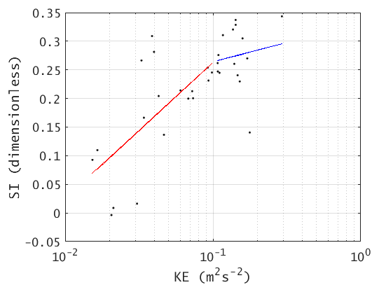
Figure B2Summer (MJJAS) KE vs. SI averaged over the box region in Fig. B1 (overall R=0.7175, p<0.01).
Dynamically, the nonlinear advection term in the momentum equation can be written as the vector-invariant form (see, e.g., Gill, 1982):
This decomposition directly links the nonlinear advection term and the gradient of KE (which scales KE over a length scale L). Meanwhile, the nonlinear advection is an important mechanism in driving flow separation (see, for instance, Oey et al., 2014). Stronger advection suggests intense cross-isobath flow. Therefore, a dynamic linkage between the flow separation and the intensified KE and circulation can also be established, further supporting this argument.
The supplement related to this article is available online at: https://doi.org/10.5194/os-14-1303-2018-supplement.
WL, EL, and YJ conceived the research, conducted the numerical calculation, and drafted the manuscript. LYO interpreted the results, designed the experiments, and revised the manuscript. WZ contributed to discussing and analyzing the results. XHY contributed to improving the manuscript. All co-authors contributed to integrating the study, and writing and refining the manuscript.
The authors declare that they have no conflict of interest.
This study was supported by grant no. 2016YFA0601201 from the Ministry of
Science and Technology of the People's Republic of China (MOST), and grants
41476005, 41476007, 41876004, and 41630963 from the National Natural Science
Foundation of China (NSFC). This study was also partially supported by the Fujian
Collaborative Innovation Center for Big Data Applications in Governments (2015750401)
and the Central Guide Local Science and Technology Development Projects (2017L3012).
The authors would like to thank Fei Chai for
providing the code of the CoSINE model. The authors would also like to thank the
three reviewers for their useful comments.
Edited by: Mario Hoppema
Reviewed by: A. Miguel P. Santos, Joachim Dippner, and one anonymous referee
Atlas, R., Hoffman, R. N., Ardizzone, J., Leidner, S. M., Jusem, J. C., Smith, D. K., and Gombos, D.: A cross-calibrated, multiplatform ocean surface wind velocity product for meteorological and oceanographic applications, B. Am. Meteorol. Soc., 92, 157–174, 2011.
Bakun, A.: Coastal upwelling indices, west coast of North America, 1946–71, US Dept. Commerce NOAA Tech. Rep. National Marine Fishery Service (NMFS) – Special Scientific Report –Fisheries (SSRF), Seattle, WA, USA, 1–103, 1973.
Bakun, A.: Patterns in the ocean: ocean processes and marine population dynamics, California Sea Grant, in cooperation with Centro de Investigaciones Biologicas del Noroeste, La Paz, Mexico, 1996.
Banzon, V., Smith, T. M., Chin, T. M., Liu, C., and Hankins, W.: A long-term record of blended satellite and in situ sea-surface temperature for climate monitoring, modeling and environmental studies, Earth Syst. Sci. Data, 8, 165–176, https://doi.org/10.5194/essd-8-165-2016, 2016.
Batchelor, G. K.: An Introduction to Fluid Dynamics, Cambridge University Press, New York, UK, 1967.
Behrenfeld, M. J. and Falkowski, P. G.: Photosynthetic rates derived from satellite-based chlorophyll concentration, Limnol. Oceanogr., 42, 1–20, 1997.
Bombar, D., Dippner, J. W., Doan, H. N., Ngoc, L. N., Liskow, I., Loick-Wilde, N., and Voss, M.: Sources of new nitrogen in the Vietnamese upwelling region of the South China Sea, J. Geophys. Res., 115, C06018, https://doi.org/10.1029/2008jc005154, 2010.
Bombar, D., Moisander, P. H., Dippner, J. W., Foster, R. A., Voss, M., Karfeld, B., and Zehr, J. P.: Distribution of diazotrophic microorganisms and nifH gene expression in the Mekong River plume during intermonsoon, Mar. Ecol. Prog. Ser., 424, 39–52, 2011.
Bryan, F. O., Hecht, M. W., and Smith, R. D.: Resolution convergence and sensitivity studies with North Atlantic circulation models. Part I: The western boundary current system, Ocean Model., 16, 141–159, 2007.
Chai, F., Liu, G., Xue, H., Shi, L., Chao, Y., Tseng, C.-M., Chou, W.-C., and Liu, K.-K.: Seasonal and interannual variability of carbon cycle in South China Sea: A three-dimensional physical-biogeochemical modeling study, J. Oceanogr., 65, 703–720, 2009.
Chassignet, E. P. and Marshall, D. P.: Gulf Stream separation in numerical ocean models, in: Ocean Modeling in an Eddying Regime, edited by: Hecht, M. W. and Hasumi, H., AGU, Washington, D.C., Geophys. Monogr. Ser., 177, 39–61, 2008.
Chen, G., Xiu, P., and Chai, F.: Physical and biological controls on the summer chlorophyll bloom to the east of Vietnam, J. Oceanogr., 70, 323–328, 2014.
Chen, Z., Yan, X.-H., Jo, Y.-H., Jiang, L., and Jiang, Y.: A study of Benguela upwelling system using different upwelling indices derived from remotely sensed data, Cont. Shelf Res., 45, 27–33, 2012.
Cushing, D.: Upwelling and fish production, FAO Fish. Tech. Pap, Food and Agriculture Organization of the United Nations, Rome, Italy, 84, 40, 1969.
Dai, A., Qian, T., Trenberth, K. E., and Milliman, J. D.: Changes in continental freshwater discharge from 1948 to 2004, J. Climate, 22, 2773–2792, 2009.
Dippner, J. W., Nguyen, K. V., Hein, H., Ohde, T., and Loick, N.: Monsoon-induced upwelling off the Vietnamese coast, Ocean Dynam., 57, 46–62, 2007.
Dippner, J. W., Bombar, D., Loick-Wilde, N., Voss, M., and Subramaniam, A.: Comment on “Current separation and upwelling over the southeast shelf of Vietnam in the South China Sea” by Chen et al., J. Geophys. Res.-Oceans, 118, 1618–1623, 2013.
Doan-Nhu, H., Lam, N.-N., and Dippner, J. W.: Development of Phaeocystis globosa blooms in the upwelling waters of the South Central coast of Viet Nam, J. Marine Syst., 83, 253–261, 2010.
Ekman, V. W.: On the influence of the earth's rotation on ocean-currents, Arkiv. Mat. Astron. Fys., 211, 1–52, 1905.
Gan, J. and Qu, T.: Coastal jet separation and associated flow variability in the southwest South China Sea, Deep-Sea Res. Pt. I, 55, 1–19, 2008.
Gan, J., Cheung, A., Guo, X., and Li, L.: Intensified upwelling over a widened shelf in the northeastern South China Sea, J. Geophys. Res., 114, C09019, https://doi.org/10.1029/2007jc004660, 2009.
Gill, A. E.: Atmosphere-ocean dynamics, Academic press, San Diego, CA, USA, 1982.
Griffies, S. M. and Hallberg, R. W.: Biharmonic Friction with a Smagorinsky-Like Viscosity for Use in Large-Scale Eddy-Permitting Ocean Models, Mon. Weather Rev., 128, 2935–2946, 2000.
Gruber, N., Lachkar, Z., Frenzel, H., Marchesiello, P., Munnich, M., McWilliams, J. C., Nagai, T., and Plattner, G.-K.: Eddy-induced reduction of biological production in eastern boundary upwelling systems, Nat. Geosci., 4, 787–792, 2011.
Guo, M., Chai, F., Xiu, P., Li, S., and Rao, S.: Impacts of mesoscale eddies in the South China Sea on biogeochemical cycles, Ocean Dynam., 65, 1335–1352, https://doi.org/10.1007/s10236-015-0867-1, 2015.
Haidvogel, D. B., McWilliams, J. C., and Gent, P. R.: Boundary Current Separation in a Quasigeostrophic, Eddy-resolving Ocean Circulation Model, J. Phys. Oceanogr., 22, 882–902, 1992.
Hein, H., Hein, B., Pohlmann, T., and Long, B. H.: Inter-annual variability of upwelling off the South-Vietnamese coast and its relation to nutrient dynamics, Global Planet. Change, 110, 170–182, 2013.
Isoguchi, O. and Kawamura, H.: MJO-related summer cooling and phytoplankton blooms in the South China Sea in recent years, Geophys. Res. Lett., 33, L16615, https://doi.org/10.1029/2006gl027046, 2006.
Jiang, Y. W., Chai, F., Wan, Z. W., Zhang, X., and Hong, H. S.: Characteristics and mechanisms of the upwelling in the southern Taiwan Strait: a three-dimensional numerical model study, J. Oceanogr., 67, 699–708, 2011.
Jiao, N., Zhang, Y., Zhou, K., Li, Q., Dai, M., Liu, J., Guo, J., and Huang, B.: Revisiting the CO2 “source” problem in upwelling areas – a comparative study on eddy upwellings in the South China Sea, Biogeosciences, 11, 2465–2475, https://doi.org/10.5194/bg-11-2465-2014, 2014.
Kalnay, E., Kanamitsu, M., Kistler, R., Collins, W., Deaven, D., Gandin, L., Iredell, M., Saha, S., White, G., and Woollen, J.: The NCEP/NCAR 40-year reanalysis project, B. Am. Meteorol. Soc., 77, 437–471, 1996.
Kuo, N.-J., Zheng, Q., and Ho, C.-R.: Satellite observation of upwelling along the western coast of the South China Sea, Remote Sens. Environ., 74, 463–470, 2000.
Kuo, N.-J., Zheng, Q., and Ho, C.-R.: Response of Vietnam coastal upwelling to the 1997–1998 ENSO event observed by multisensor data, Remote Sens. Environ., 89, 106–115, 2004.
Large, W. G., McWilliams, J. C., and Doney, S. C.: Oceanic vertical mixing: A review and a model with a nonlocal boundary layer parameterization, Rev. Geophys., 32, 363–404, 1994.
Li, Q. P., Wang, Y., Dong, Y., and Gan, J.: Modeling long-term change of planktonic ecosystems in the northern South China Sea and the upstream Kuroshio Current, J. Geophys. Res.-Oceans, 120, 3913–3936, 2015.
Liao, E., Jiang, Y., Li, L., Hong, H., and Yan, X.: The cause of the 2008 cold disaster in the Taiwan Strait, Ocean Model., 62, 1–10, https://doi.org/10.1016/j.ocemod.2012.11.004, 2013.
Lin, X., Yan, X.-H., Jiang, Y., and Zhang, Z.: Performance assessment for an operational ocean model of the Taiwan Strait, Ocean Model., 102, 27–44, 2016.
Liu, G. and Chai, F.: Seasonal and interannual variability of primary and export production in the South China Sea: a three-dimensional physical-biogeochemical model study, ICES J. Mar. Sci., 66, 420–431, 2009.
Liu, K.-K., Chao, S. Y., Shaw, P. T., Gong, G. C., Chen, C. C., and Tang, T. Y.: Monsoon-forced chlorophyll distribution and primary production in the South China Sea: observations and a numerical study, Deep-Sea Res. Pt. I, 49, 1387–1412, 2002.
Liu, K.-K., Atkinson, L., Quinones, R., and Talaue-McManus, L.: Biogeochemistry of Continental Margins in a Global Context, in: Carbon and nutrient fluxes in continental margins: a global synthesis, edited by: Liu, K.-K., Atkinson, L., Quiñones, R., and Talaue-McManus, L., Global Change – The IGBP Series, Springer, Berlin Heidelberg, Germany, 3–24, 2010.
Liu, W. T., Katsaros, K. B., and Businger, J. A.: Bulk parameterization of air-sea exchanges of heat and water vapor including the molecular constraints at the interface, J. Atmos. Sci., 36, 1722–1735, 1979.
Liu, X., Wang, J., Cheng, X., and Du, Y.: Abnormal upwelling and chlorophyll-aconcentration off South Vietnam in summer 2007, J. Geophys. Res. Oceans, 117, C07021, https://doi.org/10.1029/2012jc008052, 2012.
Loick-Wilde, N., Bombar, D., Doan, H. N., Nguyen, L. N., Nguyen-Thi, A. M., Voss, M., and Dippner, J. W.: Microplankton biomass and diversity in the Vietnamese upwelling area during SW monsoon under normal conditions and after an ENSO event, Prog. Oceanogr., 153, 1–15, 2017.
Loisel, H., Vantrepotte, V., Ouillon, S., Ngoc, D. D., Herrmann, M., Tran, V., Mériaux, X., Dessailly, D., Jamet, C., Duhaut, T., Nguyen, H. H., and Van Nguyen, T.: Assessment and analysis of the chlorophyll-a concentration variability over the Vietnamese coastal waters from the MERIS ocean color sensor (2002–2012), Remote Sens. Environ., 190, 217–232, 2017.
Lu, W., Yan, X.-H., and Jiang, Y.: Winter bloom and associated upwelling northwest of the Luzon Island: A coupled physical-biological modeling approach, J. Geophys. Res.-Oceans, 120, 533–546, 2015.
Lu, W., Yan, X.-H., Han, L., and Jiang, Y.: One-dimensional ocean model with three types of vertical velocities: a case study in the South China Sea, Ocean Dynam., 67, 253–262, https://doi.org/10.1007/s10236-016-1029-9, 2017.
Lu, W., Luo, Y.-W., Yan, X., and Jiang, Y.: Modeling the Contribution of the Microbial Carbon Pump to Carbon Sequestration in the South China Sea, Sci. China Earth Sci., 61, 1–11, https://doi.org/10.1007/s11430-017-9180-y, 2018.
Ma, W., Chai, F., Xiu, P., Xue, H., and Tian, J.: Modeling the long-term variability of phytoplankton functional groups and primary productivity in the South China Sea, J. Oceanogr., 69, 527–544, 2013.
Ma, W., Chai, F., Xiu, P., Xue, H., and Tian, J.: Simulation of export production and biological pump structure in the South China Sea, Geo-Mar. Lett., 34, 541–554, 2014.
Marshall, D. P. and Tansley, C. E.: An Implicit Formula for Boundary Current Separation, J. Phys. Oceanogr., 31, 1633–1638, 2001.
Mittelstaedt, E.: Upwelling regions, Landoldt-Börnstein, New Series, 3, 135–166, 1986.
Nagai, T., Gruber, N., Frenzel, H., Lachkar, Z., McWilliams, J. C., and Plattner, G. K.: Dominant role of eddies and filaments in the offshore transport of carbon and nutrients in the California Current System, J. Geophys. Res.-Oceans, 120, 5318–5341, 2015.
NASA/GSFC/NOAA: Cross-Calibrated Multi-Platform Ocean Surface Wind Vector L3.0 First-Look Analyses, Ver. 1, PO.DAAC, CA, USA, https://doi.org/10.5067/CCF30-01XXX, 2009.
Ning, X., Chai, F., Xue, H., Cai, Y., Liu, C., and Shi, J.: Physical-biological oceanographic coupling influencing phytoplankton and primary production in the South China Sea, J. Geophys. Res.-Oceans, 109, C10005, https://doi.org/10.1029/2004jc002365, 2004.
O'Brien, J. J. and Hurlburt, H.: A numerical model of coastal upwelling, J. Phys. Oceanogr., 2, 14–26, 1972.
Oey, L.-Y., Chang, Y.-L., Lin, Y.-C., Chang, M.-C., Varlamov, S., and Miyazawa, Y.: Cross flows in the Taiwan Strait in winter, J. Phys. Oceanogr., 44, 801–817, 2014.
Pelegrí, J. L., Arístegui, J., Cana, L., González-Dávila, M., Hernández-Guerra, A., Hernández-León, S., Marrero-Díaz, A., Montero, M. F., Sangrà, P., and Santana-Casiano, M.: Coupling between the open ocean and the coastal upwelling region off northwest Africa: water recirculation and offshore pumping of organic matter, J. Marine Syst., 54, 3–37, 2005.
Shchepetkin, A. and McWilliams, J.: The regional oceanic modeling system (ROMS): a split-explicit, free-surface, topography-following-coordinate oceanic model, Ocean Model., 9, 347–404, 2005.
Steemann-Nielsen, E. and Jensen, E. A.: Primary oceanic production, Autotrophic Prod. Organic Matter Oceans, 1, 49–135, 1957.
Tang, D. L., Kawamura, H., Doan-Nhu, H., and Takahashi, W.: Remote sensing oceanography of a harmful algal bloom off the coast of southeastern Vietnam, J. Geophys. Res.-Oceans, 109, C03014, https://doi.org/10.1029/2003jc002045, 2004.
Voss, M., Bombar, D., Loick, N., and Dippner, J. W.: Riverine influence on nitrogen fixation in the upwelling region off Vietnam, South China Sea, Geophys. Res. Lett., 33, L07604, https://doi.org/10.1029/2005gl025569, 2006.
Wang, G., Chen, D., and Su, J.: Generation and life cycle of the dipole in the South China Sea summer circulation, J. Geophys. Res., 111, C06002, https://doi.org/10.1029/2005jc003314, 2006.
Wang, J., Hong, H., Jiang, Y., Chai, F., and Yan, X.-H.: Summer nitrogenous nutrient transport and its fate in the Taiwan Strait: A coupled physical-biological modeling approach, J. Geophys. Res.-Oceans, 118, 4184–4200, 2013.
Wang, J., Hong, H., and Jiang, Y.: A coupled physical–biological modeling study of the offshore phytoplankton bloom in the Taiwan Strait in winter, J. Sea Res., 107, 12–24, 2016.
Wong, G. T. F., Ku, T. L., Mulholland, M., Tseng, C. M., and Wang, D. P.: The SouthEast Asian time-series study (SEATS) and the biogeochemistry of the South China Sea – An overview, Deep-Sea Res. Pt. II, 54, 1434–1447, 2007.
Wyrtki, K.: Physical Oceanography of the Southeast Asian waters, in: Scientific Results of Marine Investigations of the South China Sea and the Gulf of Thailand 1959–1961, NAGA report, vol. 2, Scripps Institution of Oceanography, UC San Diego, La Jolla, CA, USA, 1961.
Xie, S. P., Xie, Q., Wang, D., and Liu, W. T.: Summer upwelling in the South China Sea and its role in regional climate variations, J. Geophys. Res.-Oceans, 108, 3261, https://doi.org/10.1029/2003JC001867, 2003.
Xie, S.-P., Hu, K., Hafner, J., Tokinaga, H., Du, Y., Huang, G., and Sampe, T.: Indian Ocean capacitor effect on Indo-western Pacific climate during the summer following El Niño, J. Climate, 22, 730–747, 2009.
Xiu, P. and Chai, F.: Connections between physical, optical and biogeochemical processes in the Pacific Ocean, Prog. Oceanogr., 122, 30–53, 2014.
Xu, X., Qiu, Z., and Chen, H.: The general descriptions of the horizontal circulation in the South China Sea, in: Proceedings of the Symposium of the Chinese Society of Marine Hydrology and Meteorology, Chinese Society of Oceanology and Limno, Science Press, Beijing, China, 137–145, 1982.
Yang, H. and Wu, L.: Trends of upper-layer circulation in the South China Sea during 1959–2008, J. Geophys. Res.-Oceans, 117, C08037, https://doi.org/10.1029/2012jc008068, 2012.
Yoshida, K. and Mao, H.-L.: A theory of upwelling of large horizontal extent, J. Marine Syst., 16, 40–54, 1957.