the Creative Commons Attribution 4.0 License.
the Creative Commons Attribution 4.0 License.
 | 21 Dec 2018
Hydrography, transport and mixing of the West Spitsbergen Current: the Svalbard Branch in summer 2015
Eivind Kolås
Measurements of ocean currents, stratification and microstructure were made in August 2015, northwest of Svalbard, downstream of the Atlantic inflow in Fram Strait in the Arctic Ocean. Observations in three sections are used to characterize the evolution of the West Spitsbergen Current (WSC) along a 170 km downstream distance. Two alternative calculations imply 1.5 to 2 Sv (1 Sv = 106 m3 s−1) is routed to recirculation and Yermak branch in Fram Strait, whereas 0.6 to 1.3 Sv is carried by the Svalbard branch. The WSC cools at a rate of 0.20 ∘C per 100 km, with associated bulk heat loss per along-path meter of W m−1, corresponding to a surface heat loss of 380–550 W m−2. The measured turbulent heat flux is too small to account for this cooling rate. Estimates using a plausible range of parameters suggest that the contribution of diffusion by eddies could be limited to one half of the observed heat loss. In addition to shear-driven mixing beneath the WSC core, we observe energetic convective mixing of an unstable bottom boundary layer on the slope, driven by Ekman advection of buoyant water across the slope. The estimated lateral buoyancy flux is O(10−8) W kg−1, sufficient to maintain a large fraction of the observed dissipation rates, and corresponds to a heat flux of approximately 40 W m−2. We conclude that – at least in summer – convectively driven bottom mixing followed by the detachment of the mixed fluid and its transfer into the ocean interior can lead to substantial cooling and freshening of the WSC.


The Arctic Ocean contributes to the global ocean thermohaline circulation through exchanges in Fram Strait, which is the main connection to the Atlantic Ocean (Aagaard et al., 1985). The total volume transport through Fram Strait is 9±2 Sv (1 Sv = 106 m3 s−1) northward and 12±1 Sv southward (Fahrbach et al., 2001; Schauer et al., 2004). A large fraction of the northward flow is the West Spitsbergen Current (WSC), located on the eastern side of Fram Strait, which is a northward-flowing extension of the Norwegian Atlantic Current. The mean net volume transport in the WSC, measured along an array at 78∘50′ N in the period between 1997 and 2010, is 6.6±0.4 Sv (Beszczynska-Möller et al., 2012), of which 3.0±0.2 Sv is Atlantic Water (AW) with a temperature above 2 ∘C. The WSC continues as a topographically guided boundary current, contributing to the circumpolar boundary current downstream. Between Fram Strait and the Lomonosov Ridge, the boundary current slows down from about 0.25 to 0.06 m s−1 and changes structure from a mainly barotropic flow to a baroclinic flow (Pnyushkov et al., 2015). AW transported by the WSC is the major heat and salinity source for the Arctic Ocean (Aagaard et al., 1985; Boyd and D'Asaro, 1994; Rudels et al., 2015), and Arctic conditions are highly influenced by changes in the AW inflow properties (Polyakov et al., 2017).
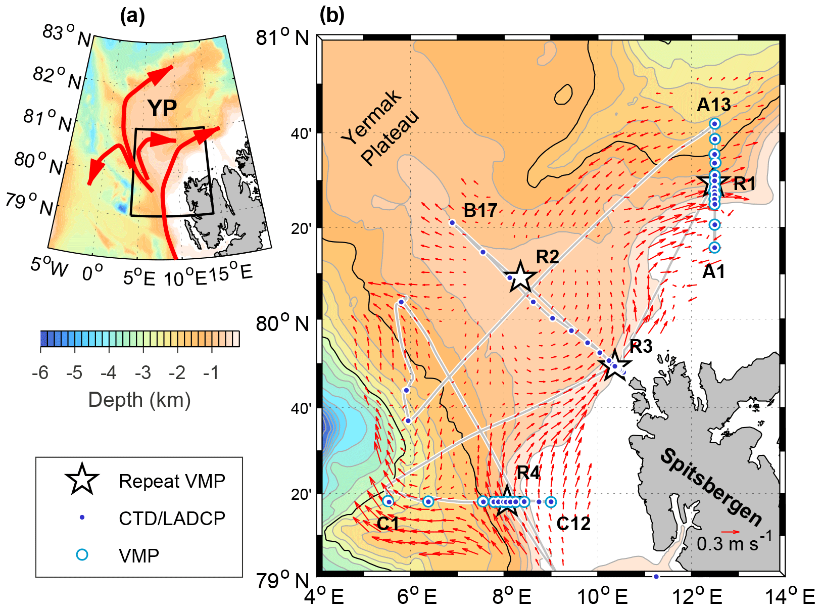
Figure 1(a) Overview map with the AW circulation patterns (red arrows). The study region zoomed in (b) is indicated by a black rectangle. (b) Station locations of sections A to C and the repeat stations R1 to R4. Selected station names at the edge of sections are marked for reference. Gray lines show the ship track during the cruise. Red arrows show the SADCP data averaged in the upper 500 m, objectively interpolated using a covariance function depending on the spatial distance between binned observations and their f∕H gradient following Böhme and Send (2005), using a 50 km correlation length scale and 5 % error.
The circulation of AW in Fram Strait has multiple branches (Fig. 1a). The WSC flows at a steady pace of approximately 0.25 m s−1, along the 1000 m isobath, from Bear Island at 74∘30′ N to the southern flanks of the Yermak Plateau (YP) at 79∘30′ N (Boyd and D'Asaro, 1994). Observations show that the WSC splits into two branches where the isobaths diverge near the YP, an outer branch following the 1000 m isobath, and an inner branch (the Svalbard branch) following the 400 m isobath (Aagaard et al., 1987; Cokelet et al., 2008; Farrelly et al., 1985). The Svalbard branch has a 40 km wide core with a strong barotropic component and flows approximately along the f∕H contours around Svalbard (Aagaard et al., 1987; Perkin and Lewis, 1984) (f is the Coriolis parameter and H is water depth). The outer branch, however, has a 60 km wide core and does not follow the 1000 m isobath as closely (Aagaard et al., 1987). Observations suggest that the outer branch splits into three different branches. A part of the flow detaches from the 1000 m isobath and recirculates in Fram Strait, contributing with warm and salty water to the southward flow on the Greenland slope (Aagaard et al., 1987; Beszczynska-Möller et al., 2012; Farrelly et al., 1985; Hattermann et al., 2016). The main recirculation is on the northern rim of the Molloy Hole at approximately 80∘ N and 4∘ E (Hattermann et al., 2016). The remaining part of the outer branch following the 1000 m isobath is called the Yermak branch and flows along the outer flanks of the YP, possibly rejoining the Svalbard branch where the isobaths converge north of Svalbard at approximately 80∘30′ N and 13∘ E (Cokelet et al., 2008; Meyer et al., 2016; Perkin and Lewis, 1984; Våge et al., 2016). Acoustically tracked subsurface floats revealed a shortcut across the YP (Gascard et al., 1995), through a topographic passage at 80∘45′ N and 6∘ E. The presence of the Yermak Pass branch is supported by numerical model results, showing flow of AW following the 700–800 m isobaths before rejoining the Svalbard branch (Koenig et al., 2017).
The outer branch was reported to contain eddies with diameters of approximately 20 km that are shed where the two branches split (Padman and Dillon, 1991; Perkin and Lewis, 1984). These eddies may control the amount of the AW recirculation in Fram Strait and, therefore, play a major role in the salt and heat budget of the Arctic Ocean (Hattermann et al., 2016; von Appen et al., 2016).
As the AW flows toward the Arctic Ocean, its salinity and temperature properties change as a result of interactions with the atmosphere and sea ice and mixing with the surrounding waters. Notable studies reporting the observed property changes in WSC are from observations from a winter cruise in January–February 1989 (Boyd and D'Asaro, 1994), from a fall cruise in October–November 2001 (Cokelet et al., 2008) and from an analysis of a 50-year hydrography data set (1949–1999), reported for summer (August–October) and winter (March–May) seasons (Saloranta and Haugan, 2004). Estimates of along-path freshening of the WSC, measured on the practical salinity scale, are 0.013∕100 km in fall 2001 (Cokelet et al., 2008) and 0.010∕100 km in summer (Saloranta and Haugan, 2004). The summer/fall cooling rate is 0.19∘ C/100 km (Cokelet et al., 2008) and 0.20∘ C/100 km (Saloranta and Haugan, 2004). The cooling rate in winter is 0.4–0.5 ∘C/100 km (Boyd and D'Asaro, 1994) and 0.31 ∘C/100 km (Saloranta and Haugan, 2004). Assuming an AW layer between 100 and 500 m depth, the cooling rate is equivalent to a heat loss of 310–330 W m−2 in summer (Aagaard et al., 1987; Cokelet et al., 2008; Saloranta and Haugan, 2004) and 1050 W m−2 in winter (Saloranta and Haugan, 2004). The cooling of the WSC stream tube observed in winter 1989 implies approximately 900 W m−2, limited to a 22 km wide core (Boyd and D'Asaro, 1994). Note that these heat losses are dependent on the mean advective speed, that is the residence time of the water in the area of cooling.
Boyd and D'Asaro (1994) describe the cooling of the WSC in winter as a three-stage process: cooling by the atmosphere, cooling by sea ice and cooling by eddy-driven mixing along isopycnals. The relative role of the different cooling processes is not clear. Numerical linear stability analyses using idealized current profile and topography suggest that heat loss contribution from isopycnal diffusion as a result of barotropic instability corresponds to an along-shelf cooling rate of 0.08 ∘C/100 km (Teigen et al., 2010). The extension of the analysis to a two-layer model shows that the baroclinic instability occurs, most pronounced during winter/spring, leading to a heat loss reaching 240 W m−2, from the core of the WSC to the atmosphere (Teigen et al., 2011).
All these studies agree that vertical mixing alone cannot account for the observed cooling rates. Fer et al. (2010) conclude that internal-wave activity and mixing show variability related to topography and hydrography; thus, the path of the WSC will affect the cooling and freshening rates the AW experiences. Over the steep slopes and prominent topography of the YP, and over the core of the AW branches, vertical mixing can play an important role in modifying the AW properties (Meyer et al., 2016; Padman and Dillon, 1991; Sirevaag and Fer, 2009). In the surface mixed layer in proximity to the WSC, turbulent heat fluxes of O(100) W m−2 were measured (Sirevaag and Fer, 2009). Once the AW subducts, the vertical mixing is suppressed by the overlaying strong stratification, reducing the heat loss to the atmosphere or sea ice. Padman and Dillon (1991) observed a time-averaged upward heat flux in the pycnocline above the Atlantic layer of 25 W m−2 over the YP slope, of which only about 6 W m−2 actually entered the mixed layer. At the core of the Svalbard branch, Fer et al. (2010) observed that near-bottom mixing removed 15 W m−2 from the AW layer to cold waters below. Outside the WSC, near the northeastern flank of the YP, Sirevaag and Fer (2009) found an average vertical heat flux of 2 W m−2, comparable to the annual oceanic heat flux of 3–4 W m−2 to the Arctic pack ice (Krishfield and Perovich, 2005).
Here we report summer observations of ocean stratification, currents and microstructure from north of Svalbard near the YP, collected during a cruise in August 2015. Using three sections across the WSC, we present the background currents, volume and heat transport and their evolution along the path of WSC. Vertical mixing and heat loss from the WSC are quantified. The goal of this study is to improve the general understanding of processes modifying the Atlantic Water inflow into the Arctic Ocean and to describe the importance of vertical mixing versus horizontal processes during summer. We propose that convective mixing in the bottom boundary layer and the subsequent lateral export of mixed water can make a substantial contribution to the cooling rate of the WSC.
The data set analyzed in this study was collected from the research vessel (R/V) Håkon Mosby between 12 and 21 August 2015. The ship track and the locations of the different stations are shown in Fig. 1b. Data were collected mainly along three sections, referred to as sections A–C, using the conductivity–temperature–depth (CTD) and lowered acoustic Doppler current profiler (LADCP) system, the vertical microstructure profiler (VMP) and the shipboard acoustic Doppler current profiler (SADCP). The sampling duration of sections A–C was approximately 20, 11 and 20 h, respectively. It took 5 days from the sampling started on section A to the end of C. Our results discussed in Sect. 4 assume that the conditions of the inner branch of the WSC do not change significantly during these 5 days, thus giving a synoptic view. In total, 46 CTD/LADCP and 85 VMP profiles are analyzed.
2.1 Temperature and salinity measurements
The CTD profiles were acquired using a Sea-Bird Scientific, SBE 911plus system. A 200 kHz Benthos altimeter allowed profiles to within 10 m of the seabed. The CTD system was also equipped with a WET Labs C-Star transmissometer. Accuracy of the pressure, temperature and salinity sensors are ±0.5 dbar, ∘C and , respectively. The CTD data are processed using the SBE software following the recommended procedures. Conservative temperature, Θ, and absolute salinity, SA, are calculated using the thermodynamic equation of seawater (IOC et al., 2010), and the Gibbs SeaWater (GSW) Oceanographic Toolbox (McDougall and Barker, 2011).
2.2 Current measurements
Horizontal current profile measurements were made using the LADCP and SADCP systems. All current measurements are corrected for the magnetic declination. Two 300 kHz Teledyne RD Instruments Workhorse LADCPs were installed on the CTD rosette collecting 1 s profiles in master–slave mode to ensure synchronization. The sampling vertical bin size was set to 8 m for each acoustic Doppler current profiler (ADCP). The LADCP data are processed as 8 m vertical averages using both ADCPs and both up- and downcasts, and using the Lamont-Doherty Earth Observatory (LDEO) Software version IX.12, which is an implementation of the velocity inversion method described in Visbeck (2002). Profiles are obtained using the constraints from velocities from ship navigation, bottom tracking and SADCP, with a resulting horizontal velocity error of less than 3 cm s−1 (Thurnherr, 2010).
SADCP on R/V Håkon Mosby was a 75 kHz Teledyne RD Instruments Ocean Surveyor. It collected velocity profiles continuously in the broadband mode. Final profiles, 5 min time-averaged, are obtained using the University of Hawaii software (Firing et al., 1995). Typical final processed horizontal velocity uncertainty is 2–3 cm s−1.
2.3 Microstructure measurements
Ocean microstructure measurements were made using a 2000 m rated VMP manufactured by Rockland Scientific, Canada (RSI). The VMP is a loosely tethered profiler with a nominal sink velocity of 0.6 m s−1. The profiler was equipped with pumped SBE-CT sensors, a pressure sensor, microstructure velocity shear probes, one high-resolution temperature sensor, one high-resolution micro-conductivity sensor and three accelerometers.
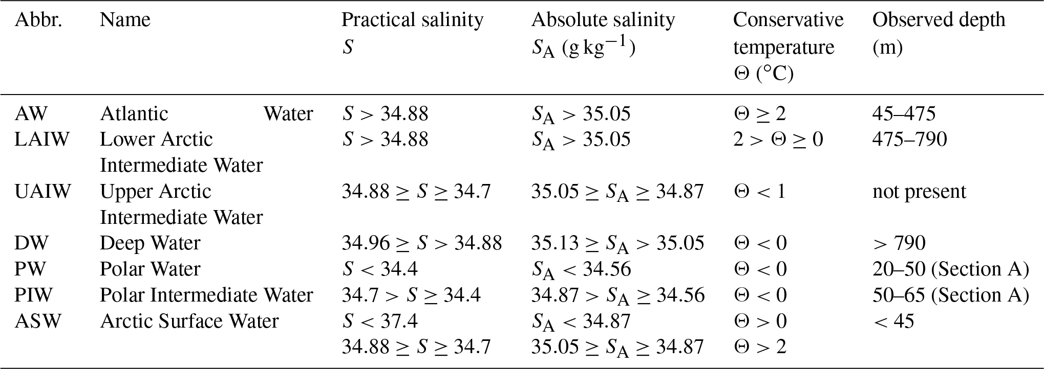
Table 1Water masses as defined by Swift and Aagaard (1981) and Aagaard et al. (1985). Absolute salinity (SA) is calculated from the practical salinity (S) at 80∘ N and 10∘ E and rounded to the nearest hundredth. The last column is the depth range of the different water masses observed in this study.
The processing of the microstructure data is based on the routines provided by RSI (ODAS v4.01) (Douglas and Lueck, 2015). Assuming isotropic turbulence, the dissipation rate of turbulent kinetic energy (TKE) per unit mass can be expressed as
where ν is the kinematic viscosity, overbar denotes averaging in time and the is the small-scale shear of one horizontal velocity component u. Using a constant fall rate of the instrument and invoking the frozen turbulence hypothesis over an analysis time of several seconds, the term with the overbar represents the shear variance from order 1 m vertical scale to order 1 cm scales where dissipation occurs. Dissipation rates are calculated from the shear variance obtained by integrating the shear wave number spectra, using 1 s Fourier transform length length and half-overlapping 4 s segments, following the corrections and methods described in the RSI Technical Notes (https://rocklandscientific.com/support/knowledge-base/technical-notes/, last access: 2 July 2018). Resulting values are quality-screened by inspecting the instrument accelerometer records and individual spectra from the two shear probes. Estimates from both probes are averaged when they agree to within a factor of 10. Otherwise, the lower dissipation value is accepted because larger values can be caused by spikes induced, e.g., by impact with plankton.
3.1 Water masses
We use the classical categorization of water masses in the region, as first defined by Swift and Aagaard (1981) and later modified by Aagaard et al. (1985), listed in Table 1. Note, however, that changes in the properties and distribution of the intermediate and deep waters in Fram Strait were observed, and discussed in Langehaug and Falck (2012). The absolute salinity, SA, in Table 1 is calculated from the practical salinity values at 80∘ N and 10∘ E and rounded to the nearest hundredth.
3.2 Tidal currents and geostrophic currents
The barotropic tidal current components in the LADCP and SADCP profiles are removed using the 5 km horizontal resolution Arctic Ocean Tidal Inverse Model, AOTIM-5 (Padman and Erofeeva, 2004). The tidal transport at specified latitude and longitude coordinates is predicted for the mid-time of the current profiles, and the barotropic tidal current is obtained by dividing by the water depth at that specific location. At the CTD/LADCP stations (Fig. 1), where station depth is accurately measured, the measured station depth is used. The water depth elsewhere (for SADCP) is obtained from the International Bathymetric Chart of the Arctic Ocean (IBCAO) database (Jakobsson et al., 2012).
Hydrography and current profiles collected along the three sections are gridded to 2 m vertical and 1 km horizontal distance, using linear interpolation. After uniformly gridding the data, a moving average smoothing is performed using a 10 km × 10 m (horizontal × vertical) window. While the smoothing removes the short timescale and length scale variability, it does not necessarily remove all ageostrophic variability.
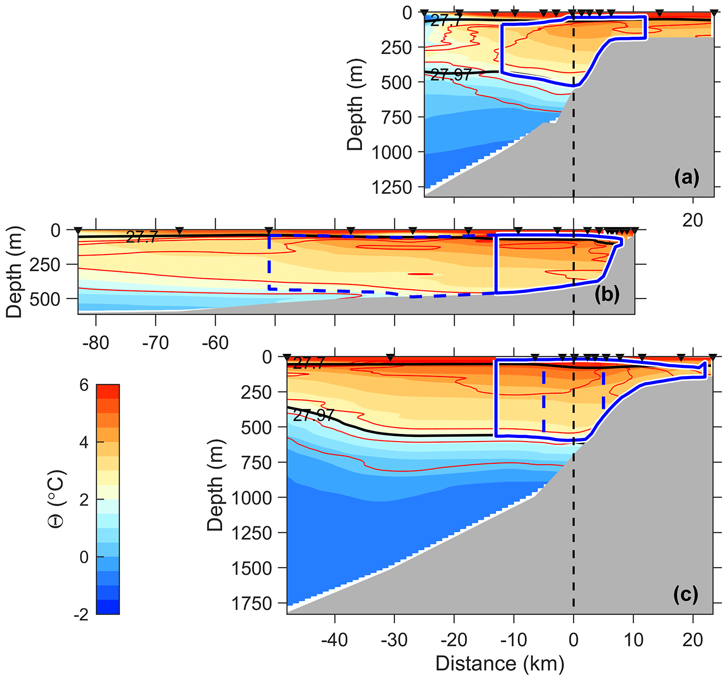
Figure 2Distribution of conservative temperature (Θ, color) and absolute salinity (SA, red contours in 0.05 g kg−1 intervals) along sections (a) A, (b) B and (c) C. Blue lines enclose stream tube 1 (solid) and stream tube 2 (dashed). Black lines are potential density anomaly, σθ, of 27.7 and 27.97 kg m−3. The horizontal distance is referenced to the core (x=0), and the three sections are aligned at x=0 (vertical dashed line). Station locations are marked with black arrows at the top of each panel.
Dynamic height anomaly and the geostrophic currents are calculated relative to a reference pressure of 100 dbar from the gridded and smoothed SA and Θ fields. The reference pressure is chosen so that it is away from frictional boundary layers where ageostrophic currents can be substantial. The absolute geostrophic velocity is then obtained by adding the across-section component of the observed currents at the reference level. The observed currents used are the de-tided LADCP profiles, identically gridded and smoothed as the hydrographic fields for consistency.
3.3 Stream tubes
The stream tube of WSC is defined using the absolute geostrophic velocities in the AW layer. The vertical extent of the tube is defined by the AW layer (or seabed). The horizontal center of the stream tube on a section is defined as the location of the maximum layer-integrated velocity (i.e., transport density, m2 s−1) and assigned x=0 km (see Figs. 5 and 6). The lateral extent of the stream tube is defined in two alternative ways.
In the first alternative (stream tube 1), the horizontal bounds are identified on either side of the core, as the location where the transport density first drops below a background threshold (solid enclosed curves in Figs. 2–4). The threshold for the transport density at each horizontal grid point is calculated by multiplying the AW layer thickness with 0.04 m s−1 (i.e., a current estimate above the ADCP measurement error of 0.03 m s−1). Sensitivity to this choice is tested using 0.02 and 0.08 m s−1. The outer stations collected by the LADCP at Section C are separated by approximately 20 km, and the linear interpolation results in currents that deviate substantially from the SADCP observations (Fig. 5c). The depth-averaged currents from the SADCP better resolve the lateral structure, off-slope away from the core. Hence for the stream tube in Section C, we use an outer bound ( km) obtained by applying the transport threshold to the SADCP velocity.
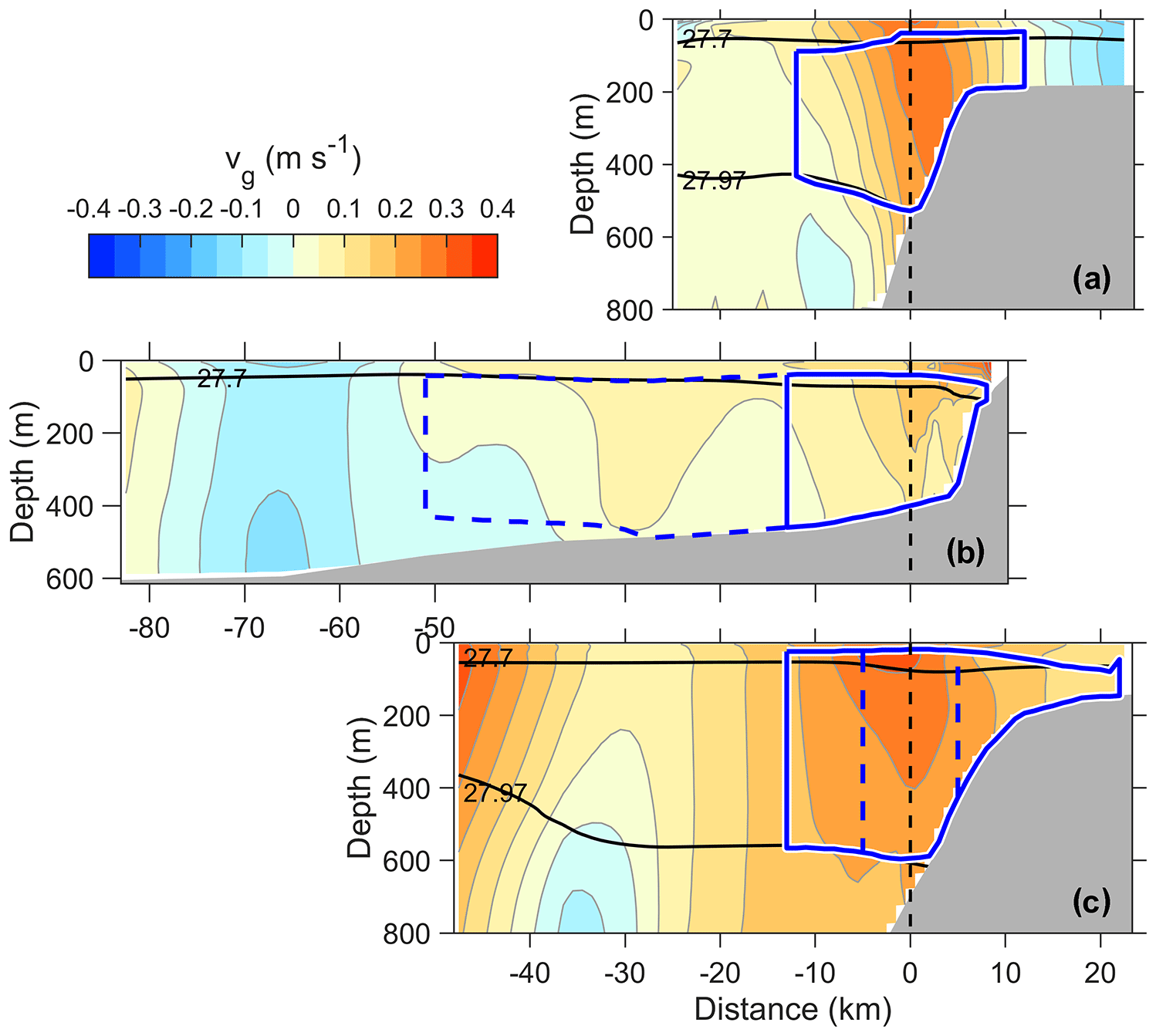
Figure 4Distribution of absolute geostrophic velocity, vg, along sections (a) A, (b) B and (c) C. Other details are as in Fig. 2.
In the second alternative (stream tube 2), we conserve the volume flux (of the Svalbard branch) in the tube to within 10 % at all sections (dashed enclosed curves in Figs. 2–4). Heat budget calculations (see Sect. 3.4) require conservation of volume. Given the 1 km horizontal resolution of our sections, and the measurement uncertainty in the velocity measurements, a conservation of volume to less than ±10 % was not practically possible. The volume flux of 1.3 Sv at Section A is deemed representative of the Svalbard branch (see Sect. 4.2) and used as a constraint in sections B and C. The lateral edges of the tube are identified by integrating the volume flux at equal horizontal distance increments centered at the core (Section B is limited by shelf).
3.4 Heat change
Neglecting molecular diffusion, the rate of change of heat content, q, of a body of fluid is balanced by the mean advection of heat and the eddy heat flux divergence
where is the horizontal velocity, an overbar denotes averaging over several eddy timescales and primes denote fluctuations. Following the method described by Boyd and D'Asaro (1994) and Cokelet et al. (2008), we integrate Eq. (2) over a fixed volume, V, to obtain
where eddy fluxes are neglected and Q and H are the heat flux to the atmosphere and sea ice, respectively. Assuming that the local heat content does not change, the surface heat flux must balance the divergence of heat. Applying the Gauss theorem on the volume integral of the heat advection yields
where the area integral is taken over the current's cross section A, is the mean temperature, is the mean velocity normal to the section, ρ0 is seawater density and CP is the specific heat capacity. Here, y is the along-path coordinate and estimated as the distance along the 500 m isobath along Spitsbergen from sections C to A (approximately 0, 86 and 171 km at sections C, B and A). We use Θ in the calculations, and the average temperature for each section is calculated as the velocity-weighted average over the stream tube. From Eq. (4), the surface heat loss per along-path meter (W m−1) from the WSC to the layer above can be estimated. The along-path temperature gradient is obtained from the slope of a line fit to three data points: along-path distance against the velocity-weighted average Θ for each section. The surface heat flux (W m−2) is then obtained by dividing the heat loss by the width of the stream tube.
3.5 Turbulent heat fluxes
The turbulent heat flux, , where w′ and T′ are the vertical velocity and temperature fluctuations, can be obtained as down-gradient diffusive flux:
where is the mean vertical temperature gradient, KT is the eddy diffusivity for heat, and the averaging and fluctuations apply to turbulent eddy scales (different from Eq. 2). Assuming that heat and density diffuse with similar coefficients in a turbulent flow (KT≈Kρ), the diapycnal eddy diffusivity can be obtained from the shear probe data using the Osborn (1980) relation
where Γ is the efficiency coefficient, ϵ is the turbulent dissipation rate and N is the buoyancy frequency. The efficiency coefficient is variable and uncertain but is commonly set to 0.2, which is the recommended value for typical oceanographic applications (Gregg et al., 2018). The heat flux is calculated from the shear measurements using Kρ with Γ=0.2 and a vertical scale of 10 m for the background temperature and density gradients.
4.1 Hydrography
Conservative temperature and absolute salinity distributions in sections A–C, show the changes along the path of the WSC (Fig. 2). The stream tubes defined in Sect. 3 are outlined in the hydrographic sections. Note that Section A is the northernmost and C is the southernmost section, and the horizontal distance is referenced to the location of the WSC core.
Temperatures near the surface exceed 6 ∘C in August and decrease with depth in all three sections (Fig. 2). The northern part of Section A is close to the ice edge and is characterized by cold surface waters. Compared to past observations, conditions in August 2015 were particularly warm, not only near the surface but also in the water column. Similar conditions were observed in summer 2016 by Richter et al. (2018). In October/November 2001 the AW temperatures above 4 ∘C, west of Svalbard, were separated from the surface by colder water (Cokelet et al., 2008), similar to the observations in winter 1989 (Boyd and D'Asaro, 1994) and in September 2012 north of Svalbard (81∘30′ N, 30∘ E) (Våge et al., 2016). When compared with the Monthly Isopycnal and Mixed-layer Ocean Climatology (MIMOC) (Schmidtko et al., 2013) in August (not shown), AW temperatures in 2015 were up to 1.8 ∘C warmer. Similarly, observations made from drifting pack ice north of Svalbard in spring 2015 showed warmer and shallower AW compared to the climatology (Meyer et al., 2016). A subsurface salinity maximum between 100 and 400 m depth was found in all three sections, similar to previous studies in this region (Cokelet et al., 2008; Meyer et al., 2016; Våge et al., 2016). Compared to the climatology, the salinities were higher in all sections by 0.08–0.12 g kg−1.
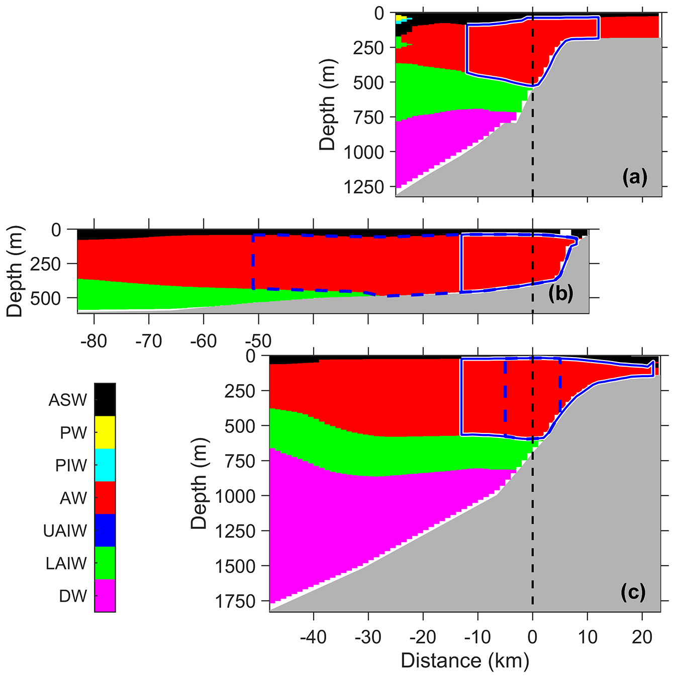
Water mass categorization (see Table 1 for definitions) shows that the AW layer overlaying LAIW extends across all sections (Fig. 3). A temperature–salinity diagram analysis following Cokelet et al. (2008) (not shown) indicates that the formation of LAIW, UAIW and DW is dominated by atmospheric cooling; i.e., the ratio of heat loss to atmosphere and to sea ice (Q∕H) exceeds 5, consistent with previous observations in winter (Boyd and D'Asaro, 1994) and autumn (Cokelet et al., 2008). In Section C, ASW is transformed by sea ice melting by AW (). In the sections farther downstream (B and A), the ASW transformation process is complex, affected by the mixing of warm and relatively fresh surface water from earlier melting events with the AW in the upper water column.
An objective analysis of temperature and salinity at 100 dbar pressure indicates that the AW properties extend along the 1000 m isobath northward. The same pattern is seen for the 100–600 m depth-averaged AW properties. However, the AW loses its depth-averaged temperature much faster than its salinity, implying mixing with colder water with similar salinity, such as LAIW (see also Kolås, 2017, for T–S diagrams).
4.2 Currents and transport
The spatial distribution of the currents measured by the SADCP helps identify the typical circulation patterns in the study region. Objectively interpolated depth-averaged currents from the SADCP show a well-defined Svalbard branch of the WSC along the 400 m isobath (Fig. 1b). The Yermak branch however, is not well-captured by the SADCP. If the Yermak branch was present in sections A and C, we would expect to see evidence of this between and km. Over the YP, there is no clear evidence of the Yermak Pass branch in this snapshot of observations. The absolute geostrophic currents toward the end of Section B (west of km), however, show currents toward the Arctic (positive values), which can be a signature of the Yermak Pass branch. This branch is expected to be variable and weak in summer (Koenig et al., 2017). Between the Svalbard branch and (possibly) the Yermak Pass branch, a barotropic current is directed southwest, centered at km (Fig. 4). North of the Molloy Hole, the currents are north–northwestward, consistent with the main recirculation route for the warmest AW (Hattermann et al., 2016).
The vertical distribution of the observed geostrophic currents along the sections captures the core of the WSC and its lateral extent (Fig. 4). The absolute geostrophic current profiles show a strong barotropic component. Sections A and C across the continental slope have a well-defined WSC core with a maximum velocity exceeding 0.3 m s−1, typically located above the 400–600 m isobath. Section B, on the other hand, extends over the YP.
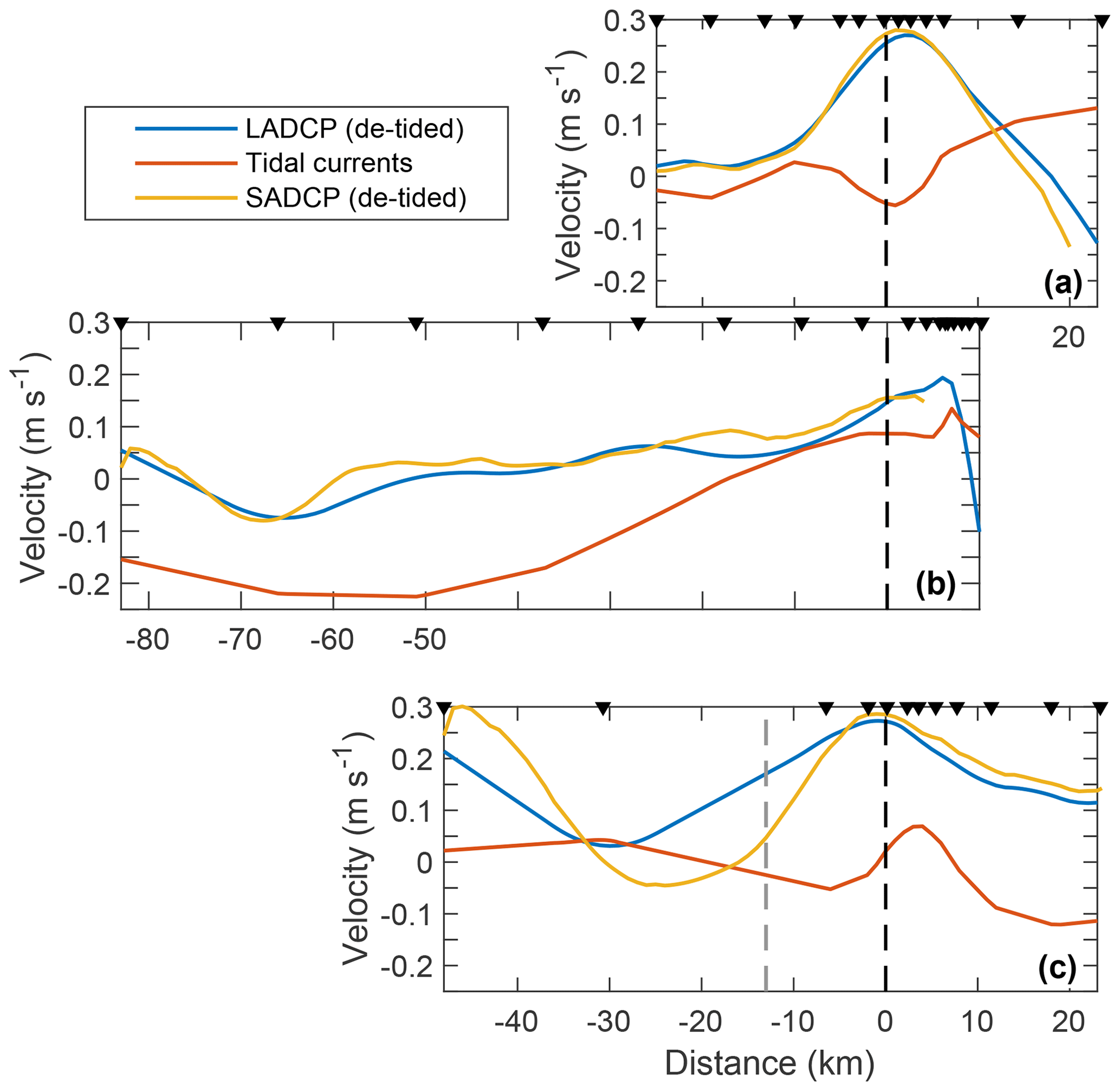
Figure 5De-tided LADCP (blue) and SADCP velocities (yellow) vertically averaged between 50 and 500 m depth and tidal currents (red) for sections A (a), B (b) and C (c). The dashed gray line at −11 km in (c) shows the outer bound of the stream tube 1 in Section C, based on SADCP measurements. Other details are as in Fig. 2.
Vertically averaged currents, between 50 and 500 m for consistency, are compared between LADCP and SADCP as well as the AOTIM5 tidal currents (Fig. 5). While the core of WSC is densely sampled by the LADCP, the coverage in the outer parts of Section C is coarse. SADCP supplements the sampling. Note the segment between and −30 km, where the rapid lateral decay of the average current is not captured by the LADCP. In Section C, therefore, the stream tube 1 outer limit is identified using the SADCP (Sect. 3.3). The agreement and coverage in other sections is good. While the currents in sections A and C are substantially more energetic than tides, Section B is characterized by strong tidal currents, particularly over the plateau between and −80 km.
Vertically integrated currents and averaged temperature and salinity show that while the salinity maximum is approximately colocated with the geostrophic velocity maximum (the core), the temperature maximum is located landward (Fig. 6). The depth-integrated velocities (volume transport per unit width) show a substantial peak at the core location (by definition) and an approximately symmetric lateral profile (Fig. 6). The lateral structure of the transport appears to be related to the location of the core relative to the slope. In sections A and C, the core is located over relatively even slopes, whereas in Section B the steep continental slope abruptly ends on the shallow YP, the current is less constrained with topography and the volume transport calculations are sensitive to the stream tube boundary definition (Table 2).
Table 2Properties in stream tubes 1 and 2 in sections A (northernmost), B and C (southernmost). The bounds for stream tube 1 given in square brackets are calculated using tube widths from the background velocity thresholds of 0.02 and 0.08 m s−1 (no bracket means no change in value). Stream tube 2 conserves a volume transport of 1.3 Sv to within 10 %. Stream tube averages, indicated by overbars, are velocity-weighted.

When the volume transport is not constrained between sections, the transport in stream tube 1 is 2.8 Sv at Section C, comparable to the previous observations. Beszczynska-Möller et al. (2012) estimated that the long-term mean net volume transport of AW between 1997 and 2010, along the array of moorings at 78∘50′ N, was 3.0±0.2 Sv. The mean transport in August, averaged over 13 years, was 2.5±0.7 Sv, with individual August averages as high as 3.6 Sv (Beszczynska-Möller et al., 2012). It should be noted that the volume transport estimated by Beszczynska-Möller et al. (2012) is roughly between the 2600 m isobath and the 300 m isobath for AW. In contrast, the tube in Section C is located between the 1100 m isobath and the 140 m isobath. Furthermore, our observation is synoptic and day-to-day or week-to-week variations are unknown.
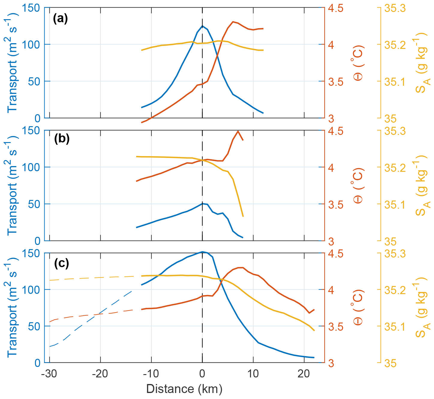
Figure 6Vertically integrated geostrophic velocity (transport per unit width; blue), and vertically averaged Θ (red) and SA (yellow) for sections (a) A, (b) B and (c) C. The horizontal distance is referenced to the core at x=0.
Progressing along path, the volume transport and velocity-weighted average temperature in stream tube 1 are 0.7 Sv and 4.18 ∘C in Section B and 1.3 Sv and 3.64 ∘C in Section A. Approximately 340 km downstream of Section A, at 81∘50′ N and 30∘ E, Våge et al. (2016) estimated an AW volume transport of 1.6±0.3 Sv in September 2012. This is larger than the transport in Section A, but the error estimates overlap. Instead of salinity, Våge et al. (2016) used a density criterion to define AW ( kg m−3 and Θ>2 ∘C), following Rudels et al. (2005). As seen in Fig. 4a, these density bounds fit the stream tube well. Våge et al. (2016) included all AW with above-zero geostrophic velocity, whereas in stream tube 1 the boundary is drawn at 0.04 m s−1; calculation using a threshold at 0.02 m s−1, however, does not lead to an increase in the total transport. The barotropic currents in Section A are landward of the 800 m isobath, whereas Våge et al. (2016) found barotropic currents 20 km seaward of the 800 m isobath. Overall, a small contribution from the Yermak branch, flowing around the tip of the plateau and joining the slope boundary current, could contribute to an increase in volume transport and explain the off-slope extent of AW in the observations of Våge et al. (2016).
If the inner branch of the WSC follows the f∕H contours and there is no synoptic variability between the sections, the partitioning of the Yermak and Svalbard branches in Section C can be estimated. The outer edge of stream tube 1 is located approximately at the 500 m isobath in Section B. The change in Coriolis parameter between sections A to C is negligible. The volume transport landward of the same isobath in Section C (tube 1) is 0.6 Sv, which is within the uncertainty of volume transport in Section B. If the stream tube 1 in Section B is representative of the topographically guided Svalbard branch of WSC, 0.6–0.7 Sv must flow through sections B toward A. Thus, the remaining 0.6–0.7 Sv could be delivered by the Yermak branch or the Yermak Pass branch in order to conserve volume. The volume transport landward of the 500 m isobath in tube 1 at Section A is 0.4 Sv, lower than sections B and C. To obtain 0.6 Sv in Section A, we have to extend the integration to a 100 m deeper isobath. Whether an event has caused the current to shift seaward or whether the divergence in current along the continental shelf break (Fig. 1, Section A) has caused a decrease in volume transport is unclear. The lack of a well-defined slope on the shelf in Section B may lead to the break of topographic control and meander the current to deeper isobaths.
In the alternative definition of stream tube 2, motivated by the well-defined core structure of WSC at Section A, we assume that the transport in Section A (defined by tube 1) is entirely the Svalbard branch, and this volume is conserved upstream at sections B and C (i.e., stream tubes 1 and 2 are identical in Section A, and the volume transport is approximately 1.3 Sv in sections B and C). This implies that Sv of AW must be routed to the Yermak branch after Section C. These figures are consistent with earlier observations and our present understanding of the AW circulation northwest of Svalbard.
4.3 Cooling and freshening of the WSC
The along-path cooling and freshening of the WSC inferred from the change in section-averaged (velocity-weighted) properties from sections C to A are similar to previous observations in summer and fall. The reduction in salinity is 0.015 g kg−1/100 km, comparable to the downstream freshening of 0.013∕100 km (on the practical salinity scale) reported by Cokelet et al. (2008) and the 50-year mean summer freshening of 0.010∕100 km, measured by Saloranta and Haugan (2004). The northward temperature gradient corresponds to a cooling rate of 0.20 ∘C/100 km for stream tube 1 and 0.23 ∘C/100 km for stream tube 2. Cokelet et al. (2008) observed 0.19 ∘C/100 km in fall 2001. Saloranta and Haugan (2004) observed a 50-year summer mean cooling rate of 0.20 ∘C/100 km, the same as that observed in 1910, between 75 and 79∘ N (Helland-Hansen and Nansen, 1912).
Calculation of the northward heat change using Eq. (4) requires the conservation of volume, which is satisfied for stream tube 2 but not in tube 1. In calculations for the tube 1, we use the transport averaged over three sections. The bounds on estimates are obtained from calculations using tube widths from the 0.02 and 0.08 m s−1 background velocity thresholds (Sect. 3.3), which reflect on velocity-weighted averages, cross section areas, as well as along-path gradients. For tube 1 we obtain an along-path heat change of , W m−1. When conserving the volume flux at 1.3 Sv, for tube 2, the heat change is W m−1. Dividing by the average tube width yields an estimate of the surface heat flux, resulting in 490 [460 550] W m−2 for tube 1 and 380 W m−2 for tube 2 (all rounded to the nearest 10 W m−2).
Boyd and D'Asaro (1994) stated that a winter heat loss per downstream meter of 2×10⁷ W m−1 (within a factor of 2) was needed to cool the warm core as much as observed, comparable to but larger than the cooling rates we observe in summer. For comparison Saloranta and Haugan (2004) estimated a summer heat loss of 330 W m−2, and Cokelet et al. (2008) reported 310 W m−2. Both studies used a mean velocity of 0.1 m s−1 when estimating the heat flux. In our observations the mean velocity was 0.15 m s−1; scaling the heat flux in tube 1 by a factor of 1.5 yields a result comparable to that of Saloranta and Haugan (2004) and Cokelet et al. (2008).
An important point to consider when calculating the northward cooling rate is the effect of the seasonal temperature cycle. Using mooring observations in Fram Strait, von Appen et al. (2016) obtain a seasonal signal with temperatures increasing from April to September, with an amplitude of 2.5 ∘C at 75 m, decreasing to less than 1 ∘C at 250 m depth. The seasonal cycle is likely weaker below 250 m. Our stream tubes span from approximately 50 to 500 m depth. Assuming an average seasonal cycle in our stream tube temperature between 0.5 and 1 ∘C over 5 months (April to September), we can estimate the northward cooling rate expected from the seasonal cycle. Using our measured mean stream tube velocity of 0.15 m s−1, a water parcel covers the 170 km distance from sections C to A in 13 days. In addition, we used 5 days from the start of Section A until we finished Section C, during which the temperature increase due to the seasonal cycle must be accounted for. Thus, over 18 days the average stream tube temperature in Section A would be between 0.06 and 0.12 ∘C less than in Section C, corresponding to a temperature loss of 0.04 to 0.07 ∘C/100 km from the seasonal cycle alone. Moored observations also show that the rate of change in the seasonal signal is not constant but weakens with time toward September when the temperature maximum occurs. A linear seasonal temperature gradient is likely not a good fit for the 18-day duration considered here, and a temperature loss in the lower range would be representative at the time of our cruise. Overall, we estimate approximately 0.05 ∘C/100 km from the seasonal cycle, which is substantially less than the inferred cooling rate of 0.2 ∘C/100 km.
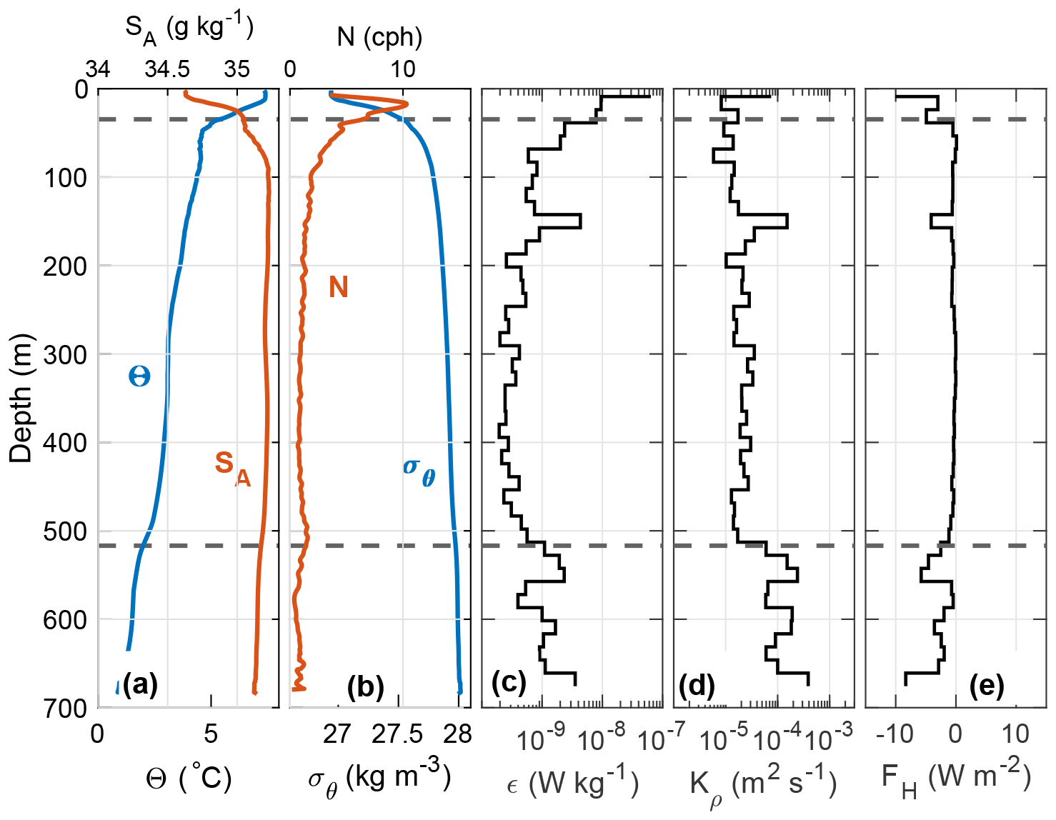
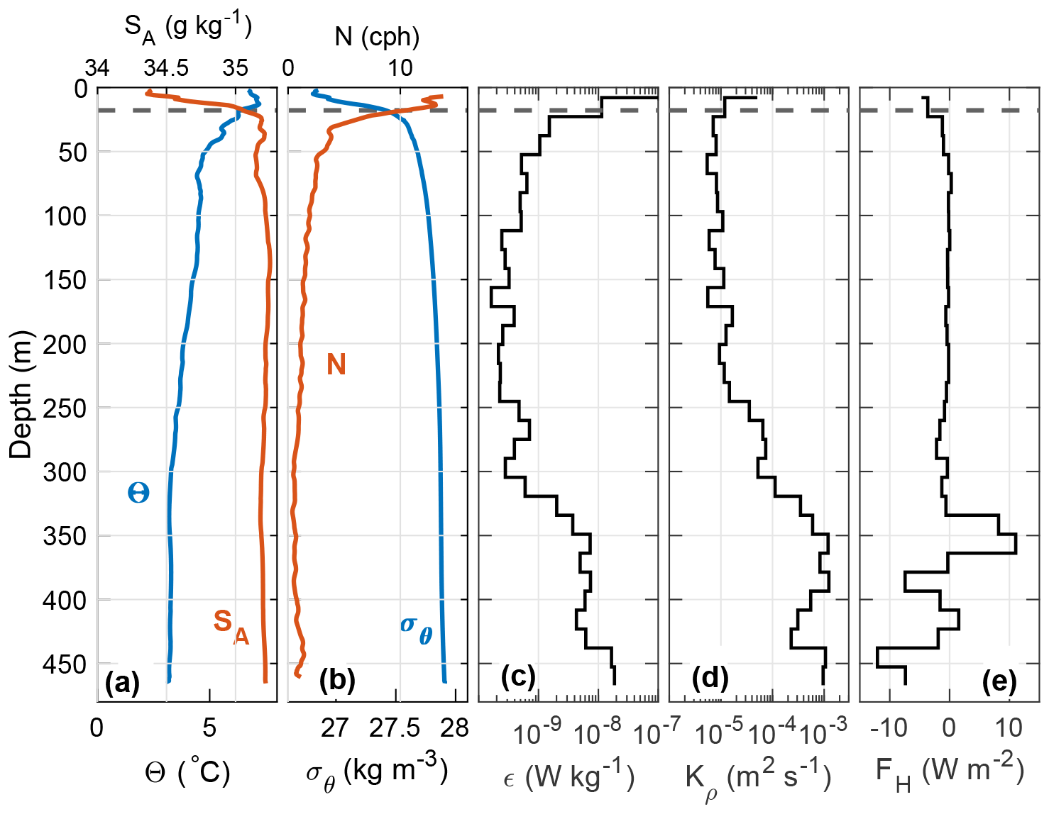
Figure 7Temporal mean of measurements collected by the microstructure profiler at station R1, Section A. (a) Θ (blue) and SA (red); (b) σθ (blue) and buoyancy frequency N (red); (c) 15 m bin-averaged dissipation of TKE ϵ; (d) eddy diffusivity Kρ; and (e) vertical heat flux FH. Dashed lines show the upper and lower boundaries of the stream tube. Water depth is 690 m.
4.4 Turbulent heat fluxes
At the time of the cruise, AW was located below the warmer and fresher ASW and above the colder LAIW. The temperature decreased with depth; hence, all vertical diffusive heat fluxes across the stream tube boundaries were negative (i.e., directed downward). Cooling by vertical heat flux is possible due to flux divergence where loss at the bottom of a layer exceeds input from the top. Figs. 7 and 8 show the temporal mean of microstructure measurements at the repeated stations R1 and R4, respectively, where the upper and lower dashed lines indicate the boundary of our stream tubes. The average profiles show a heat flux of −5 and −4 W m−2 across the upper boundary of the stream tube in R1 and R4, respectively (Figs. 7e and 8e), whereas through the bottom boundary, the heat flux is only −1 W m−2 (Fig. 7e). In sections A and C, where AW is above colder LAIW, the vertical heat flux is larger through the top of the AW layer than through the bottom, resulting in net heating. The measured average heating of AW (by vertical fluxes alone) from sections A and C is 2 and 1 W m−2, respectively. In Section B, the AW layer reaches the seabed, and the negative heat flux at the top of the layer contributes to warming the AW.
The mean turbulent heat fluxes within the AW layer are between −1 and −8 W m−2, with the largest heat flux of −39 W m−2 observed at station R3 in Section B. Away from the slope and bottom boundary layer, average heat fluxes are close to zero within the AW layer. The small fluxes north and south of the YP are consistent with previous findings in the Arctic region (Krishfield and Perovich, 2005; Sirevaag and Fer, 2009). Elevated fluxes over the YP are consistent with the observations of Padman and Dillon (1991) and Fer et al. (2010). Dissipation of TKE is small within the AW interior, only exceeding 10−8 W kg−1 in the surface and bottom boundary layer (Figs. 7 and 8c). Overall, the turbulent heat flux is too small to account for the cooling rate of the WSC inferred from our observations.
4.5 Lateral mixing and convectively driven bottom boundary layer mixing
If the AW layer is not cooled by vertical mixing, processes such as lateral mixing, shelf–basin exchange and intrusions of cold shelf water could play a role. Farther downstream, on the East Siberian continental slope, Lenn et al. (2009) argue that lateral mixing with shelf water must be one of the major causes for the observed evolution of the AW boundary current.
A mean current flowing along the slope in the direction of Kelvin wave propagation induces a downslope Ekman transport that advects lighter waters under denser waters, driving diapycnal mixing and reducing the potential vorticity (Allen and Newberger, 1998; Benthuysen and Thomas, 2012). Using detailed measurements of vertical profiles of turbulence and density through the bottom boundary layer over a sloping continental shelf, Moum et al. (2004) documented energetic convectively driven mixing induced by downwelling Ekman transport of buoyant bottom fluid.
Here we propose that convective mixing of the unstable bottom boundary layer on the slope, driven by Ekman advection of density beneath the core of the WSC, followed by the detachment of the mixed fluid and its transfer into the ocean interior (Armi, 1978) can play an important role in the modification of the WSC properties. Vigorous turbulent convection, associated with the generation of localized plumes of rising light fluid, could suspend sediments, leading to intermediate nepheloid layers – mid-depth layers of elevated suspended sediment concentration laterally advected into deep water from nearby slopes (McPhee-Shaw and Kunze, 2002). Our observations are supportive of this scenario in all three sections, and here we present details from sections C (Fig. 9) and A (Fig. 10).
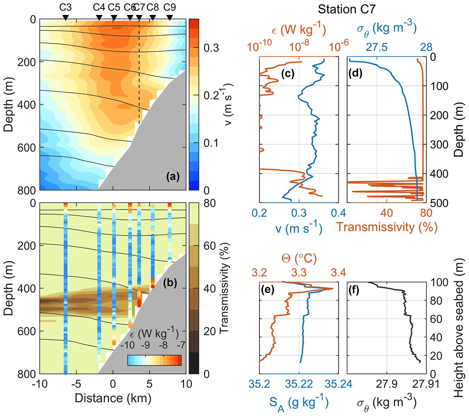
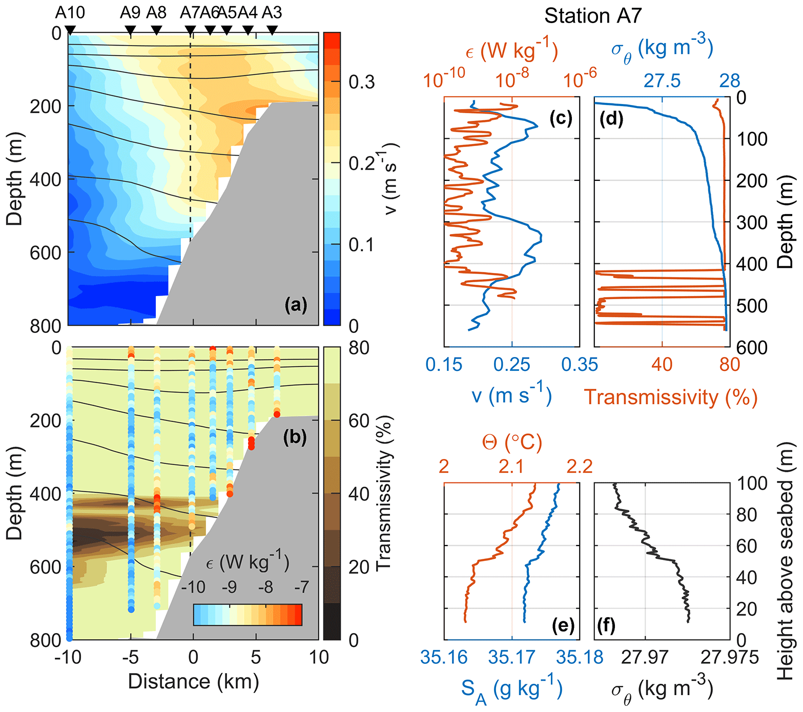
Figure 9Distribution of (a) the velocity component into the section and (b) light transmissivity, together with selected isopycnals (black). Dissipation rate (log10ϵ) is color coded in vertical columns in (b). Profiles collected at station C7: full depth profiles of (c) dissipation rate and velocity and (d) σθ and transmissivity and the bottom 100 m profiles of (e) Θ and SA and (f) σθ.
The WSC core over the slope flows in the direction of Kelvin wave propagation, and the stratification toward the shelf is characterized by less dense, relatively fresh near-bottom waters. A vertical buoyancy flux to drive convection can thus be delivered by downslope Ekman advection of buoyant water across the slope (Moum et al., 2004). Concentrated between the 400 and 600 m isobaths, the rate of dissipation is elevated near the bottom 100 m by 2 orders of magnitude above the interior levels (Figs. 9 and 10b, vertical columns). In this segment of the slope, the light transmissivity is largely reduced and extends offshore across the section (Figs. 9b and 10b, background shading). The reduction in transmissivity can be interpreted as the increase in concentration of suspended matter in the water, likely in response to vigorous turbulence and convection. The sediment-laden waters are exported laterally and isobarically and appear to cross isopycnals. The light transmissivity measurements are in situ, not calibrated and must be interpreted with caution. Nevertheless, the qualitative pattern is consistent and significant in all sections.
A vertical profile in each section, at approximately the 600 m isobath, shows the correspondence of the turbulent bottom layer with strong near-bottom shear (approximately 0.1 m s−1 over 100 m vertical distance), quasi-homogeneous bottom density and the low-transmissivity layer (Figs. 8c, d and 9c, d). A close-up of the bottommost 100 m shows that the turbulent layer is characterized by nearly well-mixed density (Figs. 9f and 10f) and a particularly weakly stratified bottom layer of approximately 40–60 m thickness with slightly colder but less saline water. On the West Spitsbergen slope, beneath the WSC core in the near-bottom layer, both shear-generated turbulence and convectively driven turbulence must play a role. Because convection fuels energy directly into the vertical component, we speculate that convection can substantially contribute to sediment suspension to yield the low-transmissivity signature we observe. Order of magnitude calculations guided by observations support this scenario.
For three adjacent stations over the slope, the vertically averaged temperature, salinity and density are calculated in the bottommost 30 m. Average density anomaly is obtained relative to the bottom 30 m vertical average. The results are comparable for all sections. The unstable density anomaly minima range between and kg m−3. The lateral gradient of the bottom-average density is to kg m−4, with temperature contributing a factor of 3 to 4.5 times more than salinity. For the observed range of density anomaly and a plausible range of vertical thickness between 10 and 80 m, Rayleigh number varies between 1010 and 1013, above the critical value of about O(103) (Turner, 1973).
The bulk stratification, N2, and shear-squared, S2, obtained from the slope of linear fits of density and velocity profiles against depth in the bottom 100 m are and 10−6 s−2, respectively, resulting in a bulk Richardson number of of 0.6. The average Ri calculated over 8 m gradients is smaller, i.e., O(0.1). We therefore expect shear-generated turbulence production, in addition to convection. When both stress and the unstable buoyancy flux produce TKE, Lombardo and Gregg (1989) show that the dissipation rate scales with a combination of the two sources. If roughly half of the dissipation is supplied by the convective buoyancy flux, the required cross-slope advection of buoyancy by bottom Ekman transport is O(10−8) W kg−1. For a range of Ekman layer thickness of 1 to 5 m (corresponding to an eddy viscosity of 10−4 to m2 s−1), an average geostrophic current of 0.3 m s−1 and the observed range of across-slope bottom-density gradient, the lateral buoyancy flux is in the range between 0.3 and W kg−1, sufficient to maintain the observed dissipation rates. When the salinity variations are negligible, the heat flux can be estimated as ρ0CPB∕(gα), where α is the thermal expansion coefficient of about 10−4 K−1 and B is the buoyancy flux. A buoyancy flux of O(10−8) W kg−1 corresponds to a vertical turbulent heat flux of approximately 40 W m−2.
The source of buoyancy is the relatively less dense waters on the shelf, maintained by the West Spitsbergen Coastal Current. The coastal current is an extension of the East Spitsbergen Current, incorporating fresh and cold PW originating from the Arctic Ocean, meltwater from glaciers, sea ice and river runoff. While the shelf waters offer a sustainable pool of buoyant water along the path of the WSC, the changes in their temperature and salinity properties would affect the resulting buoyancy flux. Substantial variability of shelf water properties are reported on short-term, interannual and long-term scales in response to changes in large-scale atmospheric patterns (Goszczko et al., 2018). The consequences of the changes in the source shelf waters on the convectively driven bottom boundary mixing and on the resulting cooling rate of the WSC merit further studies.
4.6 Isopycnal diffusion in an eddy field
In winter, an energetic eddy field diffuses heat along steeply sloping, outcropping isopycnal surfaces, at a rate sufficient to cool the subsurface warm core capped by stratification above (Boyd and D'Asaro, 1994). In winter, isopycnals in the core outcrop 5–10 km to the west of the core (Boyd and D'Asaro, 1994), whereas in our summer observations, the σθ=27.7 surface, an approximate upper bound of the AW, is relatively flat in the outer part of the sections (Fig. 2). Furthermore, the summer air temperatures are not expected to drive substantial heat loss to the atmosphere. Hence, we do not expect a large contribution from this process in summer. The lateral mixing by eddies, however, can still be substantial, depending on the dynamics of the eddy field and the structure of the isopycnals. The contribution from isopycnal diffusion as a result of barotropic instability could account for approximately one-third of the typical along-shelf cooling rate (Teigen et al., 2010). Baroclinic instability, most pronounced during winter/spring, could lead to a heat loss from the WSC core, reaching 240 W m−2 (Teigen et al., 2011). Both studies are highly idealized but suggest that isopycnal diffusion by eddies can be important. Our data set is not sufficient to provide an accurate estimate of the isopycnal diffusion by eddies.
Våge et al. (2016) observed an anticyclonic eddy with a radius of 10–15 km and a vertical scale of 250–300 m. Crews et al. (2018) analyzed 177 eddies detected over the course of 2 years using eddy-resolving numerical experiments in the region north of Svalbard. The eddies in the region can be characterized by a radius of 5–6 km, a thickness of 300 m and an average velocity anomaly of approximately 5 cm s−1, overall consistent with the limited observations. Using an eddy length scale of km and velocity perturbation of cm s−1 gives an estimate of the isopycnal diffusivity of m2 s−1. The average lateral temperature gradient of AW 0.05 ∘C per kilometer then yields an average horizontal flux of 5×10⁴ W m−2. Multiplying by a typical eddy thickness of 300 m, we obtain W m−1, lost laterally outward along the side of the stream tube. This is of the same order as the estimated along-path heat change. Assuming a fraction (0.5) of the along-path distance is affected by eddies will result in half of the heat loss unexplained, unaccounted for by interior diapycnal mixing and eddy-induced isopycnal diffusion. The cooling induced by convectively driven bottom mixing can thus be important.
Observations from a cruise conducted in August 2015 provide a snapshot of the West Spitsbergen Current (WSC) hydrography, transport and mixing in ice-free regions west and north of Svalbard in a year with relatively warmer and saltier Atlantic Water (AW) compared to climatology. Data were collected in three sections across the WSC, along an approximately 170 km long path.
The Svalbard branch of the WSC is topographically guided close to the shelf break and is relatively well captured by our observations. The recirculating branch in Fram Strait, the Yermak branch and the Yermak Pass branch are not resolved, but inferences are made from the observed sections. The volume transport in a stream tube of WSC, defined using the AW properties and along-path velocities above a background value, is 2.8 Sv in Fram Strait before the Svalbard and Yermak branches split. The transport reduces to 1.3 Sv in the most downstream section north of Svalbard. In a scenario where the Svalbard branch is constrained to the 500 m isobath in the middle section, its volume transport is 0.6–0.7 Sv, implying that approximately 2 Sv is fed to recirculation and Yermak branch in Fram Strait, and 0.6–0.7 Sv is potentially delivered by the Yermak branch or the Yermak Pass branch which could join the Svalbard branch in the northern section. An alternative scenario, assuming the transport in the most downstream section is entirely the Svalbard branch (1.3 Sv) and this volume is conserved in the sections upstream, implies that 1.5 Sv of AW must be routed to the Yermak Branch in Fram Strait.
The along-path cooling of the WSC is similar to previous observations in summer and fall, with approximately 0.20 ∘C per 100 km. The associated bulk heat loss per along-path meter is W m−1, corresponding to a surface heat flux of 380–550 W m−2. The measured turbulent heat flux is too small to account for this cooling rate. In contrast to winter conditions, we do not expect heat loss by diffusion along outcropping isopycnals. The lateral mixing by eddies, however, can be substantial, depending on the dynamics of the eddy field and the structure of the isopycnals. While our observations are not sufficient to allow an accurate quantification of the diffusion by eddies, estimates using a plausible range of parameters suggest that the contribution from eddies could be limited to one half of the observed heat loss. We propose that energetic convective mixing of the unstable bottom boundary layer on the slope, driven by Ekman advection of density beneath the core of the WSC, followed by the detachment of the mixed fluid and its transfer into the ocean interior can explain a significant part of the remaining heat loss.
The WSC core on the slope flows in the direction of Kelvin wave propagation, inducing the downslope Ekman advection. Relatively less dense near-bottom waters on the shelf are the source of buoyancy, maintained by the cold and fresh waters from the Svalbard coast and fjords joining the west Spitsbergen coastal current. Our detailed observations show turbulence generation through a combination of mean shear and convection. Downslope Ekman advection across the slope leads to a lateral buoyancy flux of O(10−8) W kg−1, sufficient to maintain a large fraction of the observed dissipation rates, and corresponds to a heat flux of approximately 40 W m2. Convectively driven bottom mixing can be important for cooling and freshening of the WSC.
The data set is available through the Norwegian Marine Data Centre: https://doi.org/10.21335/NMDC-567625440 (Fer and Kolås, 2018).
IF designed the experiment; EK and IF collected the data, conceived and planned the analysis. EK performed the analysis and wrote the paper, with advice and critical feedback from IF. Both authors discussed the results and finalized the paper.
The authors declare that they have no conflict of interest.
This study was supported by the Research Council of Norway through the
project 229786. The work is based on the MSc study of Eivind Kolås
(Kolås, 2017). We thank the crew and participants of the cruise
HM 2015617. We also thank Igor Polyakov and an anonymous reviewer for their
valuable comments that helped improve an earlier version of the paper.
Edited by: Matthew Hecht
Reviewed by: Igor Polyakov and one anonymous referee
Aagaard, K., Swift, J. H., and Carmack, E. C.: Thermohaline circulation in the Arctic Mediterranean Seas, J. Geophys. Res., 90, 4833, https://doi.org/10.1029/JC090iC03p04833, 1985. a, b, c, d
Aagaard, K., Foldvik, A., and Hillman, S. R.: The West Spitsbergen Current: Disposition and water mass transformation, J. Geophys. Res., 92, 3778–3784, https://doi.org/10.1029/JC092iC04p03778, 1987. a, b, c, d, e
Allen, J. S. and Newberger, P. A.: On Symmetric Instabilities in Oceanic Bottom Boundary Layers, J. Phys. Oceanogr., 28, 1131–1151, https://doi.org/10.1175/1520-0485(1998)028<1131:osiiob>2.0.co;2, 1998. a
Armi, L.: Some evidence for boundary mixing in the deep ocean, J. Geophys. Res., 83, 1971–1979, 1978. a
Benthuysen, J. and Thomas, L. N.: Friction and Diapycnal Mixing at a Slope: Boundary Control of Potential Vorticity, J. Phys. Oceanogr., 42, 1509–1523, https://doi.org/10.1175/jpo-d-11-0130.1, 2012. a
Beszczynska-Möller, A., Fahrbach, E., Schauer, U., and Hansen, E.: Variability in Atlantic water temperature and transport at the entrance to the Arctic Ocean, 1997–2010, ICES J. Mar. Sci., 69, 852–863, https://doi.org/10.1093/icesjms/fss056, 2012. a, b, c, d, e
Böhme, L. and Send, U.: Objective analyses of hydrographic data for referencing profiling float salinities in highly variable environments, Deep-Sea Res. Pt. II, 52, 651–664, 2005. a
Boyd, T. J. and D'Asaro, E. A.: Cooling of the West Spitsbergen Current: Wintertime Observations West of Svalbard, J. Geophys. Res., 99, 22597–22618, https://doi.org/10.1029/94JC01824, 1994. a, b, c, d, e, f, g, h, i, j, k, l
Cokelet, E. D., Tervalon, N., and Bellingham, J. G.: Hydrography of the West Spitsbergen Current, Svalbard Branch: Autumn 2001, J. Geophys. Res., 113, C01006, https://doi.org/10.1029/2007JC004150, 2008. a, b, c, d, e, f, g, h, i, j, k, l, m, n, o
Crews, L., Sundfjord, A., Albretsen, J., and Hattermann, T.: Mesoscale Eddy Activity and Transport in the Atlantic Water Inflow Region North of Svalbard, J. Geophys. Res., 123, 201–215, 2018. a
Douglas, W. and Lueck, R.: ODAS MATLAB Library. Technical Manual, Version 4.0, Tech. rep., Rockland Scientific International Inc., available at: https://rocklandscientific.com (last access: 2 July 2018), 2015. a
Fahrbach, E., Meincke, J., Østerhus, S., Rohardt, G., Schauer, U., Tverberg, V., Verduin, J., and Woodgate, R. A.: Direct measurements of heat and mass transports through the Fram Strait, Polar Res., 20, 217–224, https://doi.org/10.1111/j.1751-8369.2001.tb00059.x, 2001. a
Farrelly, B., Gammelsrød, T., Golmen, L. G., and Sjøberg, B.: Hydrographic conditions in the Fram Strait, summer 1982, Polar Res., 3, 227–238, https://doi.org/10.1111/j.1751-8369.1985.tb00509.x, 1985. a, b
Fer, I. and Kolås, E.: Ocean currents, hydrography and microstructure data from cruise HM2015617, Norwegian Marine Data Centre, https://doi.org/10.21335/NMDC-567625440, 2018. a
Fer, I., Skogseth, R., and Geyer, F.: Internal waves and mixing in the Marginal Ice Zone near the Yermak Plateau, J. Phys. Oceanogr., 40, 1613–1630, https://doi.org/10.1175/2010JPO4371.1, 2010. a, b, c
Firing, E., Ranada, J., and Caldwell, P.: Processing ADCP data with the CODAS software system version 3.1, Joint Institute for Marine and Atmospheric Research, University of Hawaii & National Oceanographic Data Center, PANGAEA, Bremerhaven, p. 226, 1995. a
Gascard, J. C., Richez, C., and Roaualt, C.: New insights on large-scale oceanography in Fram Strait: the West Spitsbergen Current, in: Arctic oceanography, marginal ice zones and continental shelves, vol. 49, chap. 5, edited by: Smith Jr., W. O. and Grebmeier, J., AGU, Washington, D.C., 131–182, 1995. a
Goszczko, I., Ingvaldsen, R. B., and Onarheim, I. H.: Wind-Driven Cross-Shelf Exchange – West Spitsbergen Current as a Source of Heat and Salt for the Adjacent Shelf in Arctic Winters, J. Geophys. Res.-Oceans, 123, 2668–2696, https://doi.org/10.1002/2017JC013553, 2018. a
Gregg, M., D'Asaro, E., Riley, J., and Kunze, E.: Mixing Efficiency in the Ocean, Annu. Rev. Mar. Sci., 10, 443–473, https://doi.org/10.1146/annurev-marine-121916-063643, 2018. a
Hattermann, T., Isachsen, P. E., Von Appen, W. J., Albretsen, J., and Sundfjord, A.: Eddy-driven recirculation of Atlantic Water in Fram Strait, Geophys. Res. Lett., 43, 3406–3414, https://doi.org/10.1002/2016GL068323, 2016. a, b, c, d
Helland-Hansen, B. and Nansen, F.: The Sea West of Spitsbergen, The Oceanographic Observations of the Isachsen Spitsbergen Expedition in 1910, Vetenskapsselskpaets Skrifter. I. Mat.-Maturv. Klasse, 12, 89, 1912. a
IOC, SCOR, and IAPSO: The international thermodynamic equation of seawater – 2010: Calculations and use of thermodynamic properties, Intergovernmental Oceanographic Commission, Manuals and Guides No. 56, Tech. rep., UNESCO, 196 pp., 2010. a
Jakobsson, M., Mayer, L., Coakley, B., Dowdeswell, J. A., Forbes, S., Fridman, B., Hodnesdal, H., Noormets, R., Pedersen, R., Rebesco, M., Schenke, H. W., Zarayskaya, Y., Accettella, D., Armstrong, A., Anderson, R. M., Beinhoff, P., Camerlenghi, A., Church, I., Edwards, M., Gerdner, J. V., Hall, J. K., Hell, B., Hestvik, O., Kristoffersen, Y., Marcussen, C., Mohammad, R., Mosher, D., Ngheim, S. V., Pedrosa, M. T., Travaglini, P. G., and Weatherall, P.: The International Bathymetric Chart of the Arctic Ocean (IBCAO) Version 3.0, Geophys. Res. Lett., 39, L12609, https://doi.org/10.1029/2012GL052219, 2012. a
Koenig, Z., Provost, C., Sennéchael, N., Garric, G., and Gascard, J. C.: The Yermak Pass Branch: A Major Pathway for the Atlantic Water North of Svalbard?, J. Geophys. Res., 122, 9332–9349, https://doi.org/10.1002/2017JC013271, 2017. a, b
Kolås, E.: The Svalbard branch of the West Spitsbergen Current: Hydrography, transport and mixing, MS thesis, University of Bergen, Bergen, available at: http://hdl.handle.net/1956/16389 (last access: 2 July 2018), 2017. a, b
Krishfield, R. A. and Perovich, D. K.: Spatial and temporal variability of oceanic heat flux to the Arctic ice pack, J. Geophys. Res., 110, 1–20, https://doi.org/10.1029/2004JC002293, 2005. a, b
Langehaug, H. R. and Falck, E.: Changes in the properties and distribution of the intermediate and deep waters in the Fram Strait, Prog. Oceanogr., 96, 57–76, https://doi.org/10.1016/j.pocean.2011.10.002, 2012. a
Lenn, Y. D., Wiles, P. J., Torres-Valdes, S., Abrahamsen, E. P., Rippeth, T. P., Simpson, J. H., Bacon, S., Laxon, S. W., Polyakov, I., Ivanov, V., and Kirillov, S.: Vertical mixing at intermediate depths in the Arctic boundary current, Geophys. Res. Lett., 36, L05601, https://doi.org/10.1029/2008GL036792, 2009. a
Lombardo, C. P. and Gregg, M. C.: Similarity scaling of viscous and thermal dissipation in a convecting boundary layer, J. Geophys. Res., 94, 6273–6284, 1989. a
McDougall, T. J. and Barker, P. M.: Getting started with TEOS-10 and the Gibbs Seawater (GSW) Oceanographic Toolbox, SCOR/IAPSO WG127, 28 pp., 2011. a
McPhee-Shaw, E. E. and Kunze, E.: Boundary layer intrusions from a sloping bottom: A mechanism for generating intermediate nepheloid layers, J. Geophys. Res., 107, 3050, https://doi.org/10.1029/2001jc000801, 2002. a
Meyer, A., Sundfjord, A., Fer, I., Provost, C., Vilacieros-Robineau, N., Koenig, Z., Onarheim, I. H., Smedsrud, L. H., Duarte, P., Dodd, P. A., Graham, R. M., Schmidtko, S., and Kauko, H. M.: Winter to summer hydrographic and current observations in the Arctic Ocean north of Svalbard, J. Geophys. Res., 122, 1–49, https://doi.org/10.1002/2016JC012391, 2016. a, b, c, d
Moum, J. N., Perlin, A., Klymak, J. M., Levine, M. D., Boyd, T., and Kosro, P. M.: Convectively driven mixing in the bottom boundary layer, J. Phys. Oceanogr., 34, 2189–2202, 2004. a, b
Osborn, T. R.: Estimates of the local rate of vertical diffusion from dissipation measurements, J. Phys. Oceanogr., 10, 83–89, 1980. a
Padman, L. and Dillon, T. M.: Turbulent mixing near the Yermak Plateau during the Coordinated Eastern Arctic Experiment, J. Geophys. Res., 96, 4769–4782, https://doi.org/10.1029/90JC02260, 1991. a, b, c, d
Padman, L. and Erofeeva, S.: A barotropic inverse tidal model for the Arctic Ocean, Geophys. Res. Lett., 31, L02303, https://doi.org/10.1029/2003GL019003, 2004. a
Perkin, R. G. and Lewis, E. L.: Mixing in the West Spitsbergen Current, J. Phys. Oceanogr., 14, 1315–1325, https://doi.org/10.1175/1520-0485(1984)014<1315:MITWSC>2.0.CO;2, 1984. a, b, c
Pnyushkov, A. V., Polyakov, I. V., Ivanov, V. V., Aksenov, Y., Coward, A. C., Janout, M., and Rabe, B.: Structure and variability of the boundary current in the Eurasian Basin of the Arctic Ocean, Deep-Sea Res. Pt. I, 101, 80–97, https://doi.org/10.1016/j.dsr.2015.03.001, 2015. a
Polyakov, I. V., Pnyushkov, A. V., Alkire, M. B., Ashik, I. M., Baumann, T. M., Carmack, E. C., Goszczko, I., Guthrie, J., Ivanov, V. V., Kanzow, T., Krishfield, R., Kwok, R., Sundfjord, A., Morison, J., Rember, R., and Yulin, A.: Greater role for Atlantic inflows on sea-ice loss in the Eurasian Basin of the Arctic Ocean, Science, 356, 285–291, https://doi.org/10.1126/science.aai8204, 2017. a
Richter, M. E., von Appen, W.-J., and Wekerle, C.: Does the East Greenland Current exist in the northern Fram Strait?, Ocean Science, 14, 1147–1165, https://doi.org/10.5194/os-14-1147-2018, 2018. a
Rudels, B., Björk, G., Nilsson, J., Winsor, P., Lake, I., and Nohr, C.: The interaction between waters from the Arctic Ocean and the Nordic Seas north of Fram Strait and along the East Greenland Current: results from the Arctic Ocean-O2 Oden expedition, J. Mar. Syst., 55, 1–30, https://doi.org/10.1016/j.jmarsys.2004.06.008, 2005. a
Rudels, B., Korhonen, M., Schauer, U., Pisarev, S., Rabe, B., and Wisotzki, A.: Circulation and transformation of Atlantic water in the Eurasian Basin and the contribution of the Fram Strait inflow branch to the Arctic Ocean heat budget, Prog. Oceanogr., 132, 128–152, https://doi.org/10.1016/j.pocean.2014.04.003, 2015. a
Saloranta, T. M. and Haugan, P. M.: Northward cooling and freshening of the warm core of the West Spitsbergen Current, Polar Res., 23, 79–88, https://doi.org/10.1111/j.1751-8369.2004.tb00131.x, 2004. a, b, c, d, e, f, g, h, i, j
Schauer, U., Fahrbach, E., Østerhus, S., and Rohardt, G.: Arctic warming through the Fram Strait: Oceanic heat transport from 3 years of measurements, J. Geophys. Res., 109, C06026, https://doi.org/10.1029/2003JC001823, 2004. a
Schmidtko, S., Johnson, G. C., and Lyman, J. M.: MIMOC: A global monthly isopycnal upper-ocean climatology with mixed layers, J. Geophys. Res., 118, 1658–1672, https://doi.org/10.1002/jgrc.20122, 2013. a
Sirevaag, A. and Fer, I.: Early Spring Oceanic Heat Fluxes and Mixing Observed from Drift Stations North of Svalbard, J. Phys. Oceanogr., 39, 3049–3069, https://doi.org/10.1175/2009JPO4172.1, 2009. a, b, c, d
Swift, J. H. and Aagaard, K.: Seasonal transitions and water mass formation in the Iceland and Greenland seas, Deep-Sea Res. Pt. A, 28, 1107–1129, https://doi.org/10.1016/0198-0149(81)90050-9, 1981. a, b
Teigen, S. H., Nilsen, F., and Gjevik, B.: Barotropic instability in the West Spitsbergen Current, J. Geophys. Res., 115, C07016, https://doi.org/10.1029/2009JC005996, 2010. a, b
Teigen, S. H., Nilsen, F., Skogseth, R., Gjevik, B., and Beszczynska-Möller, A.: Baroclinic instability in the West Spitsbergen Current, J. Geophys. Res., 116, C07012, https://doi.org/10.1029/2011JC006974, 2011. a, b
Thurnherr, A. M.: A Practical Assessment of the Errors Associated with Full-Depth LADCP Profiles Obtained Using Teledyne RDI Workhorse Acoustic Doppler Current Profilers, J. Atmos. Ocean. Tech., 27, 1215–1227, https://doi.org/10.1175/2010JTECHO708.1, 2010. a
Turner, J. S.: Buoyancy Effects in Fluids, Cambridge University Press, New York, 1973. a
Våge, K., Pickart, R. S., Pavlov, V., Lin, P., Torres, D. J., Ingvaldsen, R., Sundfjord, A., and Proshutinsky, A.: The Atlantic Water boundary current in the Nansen Basin: Transport and mechanisms of lateral exchange, J. Geophys. Res., 121, 6946–6960, https://doi.org/10.1002/2016JC011715, 2016. a, b, c, d, e, f, g, h, i
Visbeck, M.: Deep velocity profiling using lowered acoustic Doppler current profilers: Bottom track and inverse solutions, J. Atmos. Ocean. Tech., 19, 794–807, https://doi.org/10.1175/1520-0426(2002)019<0794:DVPULA>2.0.CO;2, 2002. a
von Appen, W.-J., Schauer, U., Hattermann, T., and Beszczynska-Möller, A.: Seasonal Cycle of Mesoscale Instability of the West Spitsbergen Current, J. Phys. Oceanogr., 46, 1231–1254, https://doi.org/10.1175/JPO-D-15-0184.1, 2016. a, b