the Creative Commons Attribution 4.0 License.
the Creative Commons Attribution 4.0 License.
 | 01 Jun 2018
Spatial variations in zooplankton community structure along the Japanese coastline in the Japan Sea: influence of the coastal current
Taku Wagawa
Naoki Iguchi
Yoshitake Takada
Takashi Takahashi
Ken-Ichi Fukudome
Haruyuki Morimoto
Tsuneo Goto
This study evaluates spatial variations in zooplankton community structure and potential controlling factors along the Japanese coast under the influence of the coastal branch of the Tsushima Warm Current (CBTWC). Variations in the density of morphologically identified zooplankton in the surface layer in May were investigated for a 15-year period. The density of zooplankton (individuals per cubic meter) varied between sampling stations, but there was no consistent west–east trend. Instead, there were different zooplankton community structures in the west and east, with that in Toyama Bay particularly distinct: Corycaeus affinis and Calanus sinicus were dominant in the west and Oithona atlantica was dominant in Toyama Bay. Distance-based redundancy analysis (db-RDA) was used to characterize the variation in zooplankton community structure, and four axes (RD1–4) provided significant explanation. RD2–4 only explained < 4.8 % of variation in the zooplankton community and did not show significant spatial difference; however, RD1, which explained 89.9 % of variation, did vary spatially. Positive and negative species scores on RD1 represent warm- and cold-water species, respectively, and their variation was mainly explained by water column mean temperature, and it is considered to vary spatially with the CBTWC. The CBTWC intrusion to the cold Toyama Bay is weak and occasional due to the submarine canyon structure of the bay. Therefore, the varying bathymetric characteristics along the Japanese coast of the Japan Sea generate the spatial variation in zooplankton community structure, and dominance of warm-water species can be considered an indicator of the CBTWC.
- Article
(2631 KB) -
Supplement
(69 KB) - BibTeX
- EndNote


Ocean currents transport water with heat and solved materials, and thus they are related to climate properties and distributions of dissolved and particulate matter (Thorpe, 2010). The biological importance of ocean currents has been accepted for a century, since Hjort (1914), and is especially applicable in coastal areas which only cover 7 % of the ocean but support 90 % of global fish catches (Pauly et al., 2002). Plankton community structure varies in accordance with currents (Russell, 1935), and changes in ocean currents cause fisheries' regimes to shift, such as from sardine to anchovy and back (Chavez et al., 2003). Ocean currents are important for zooplankton abundance and community structure: the Gulf Stream affects the abundance of copepods, Calanus finmarchicus and C. helgolandicus, in the European coastal seas (Frid and Huliselan, 1996; Reid et al., 2003), and the copepod species richness varies with the inflow of source water in the California current (Hooff and Peterson, 2006). Not only ocean currents but also water temperature, nutrient supply, and many other factors affect zooplankton abundance and community structure; thus, monitoring results of zooplankton abundance and community usually reflect hydro-meteorological change (Beaugrand, 2005).
In the Japan Sea (Sea of Japan), which is a marginal sea of the western North Pacific, the Tsushima Warm Current (TWC) flows from west (connected to the East China Sea at the Tsushima Strait) to east (connected to the western North Pacific and the Okhotsk Sea at the Tsugaru and Soya straits, respectively). The TWC has three branches (Kawabe, 1982): the coastal (first) branch (CBTWC) flows along the Japanese coast following the shelf edge; the second branch flows on the offshore side of the first branch; the third branch (also known as East Korean Warm Current) flows along the Korean Peninsula up to ∼ 39∘ N. The TWC transport affects climate and marine systems in the Japan Sea and the Japanese Archipelago (Hirose et al., 1996, 2009; Isobe et al., 2002; Onitsuka et al., 2010; Kodama et al., 2015, 2016), and is the spawn and nursery field of important fisheries' resources (Goto, 1998, 2002; Kanaji et al., 2009; Ohshimo et al., 2017).
Zooplankton are transported by the TWC: the distributions of the giant jellyfish, Nemopilema nomurai, which originates from the Chinese coastal area of the East China Sea (Uye, 2008; Kitajima et al., 2015), and the giant salps, Thetys vagina (Iguchi and Kidokoro, 2006), depend on the TWC in the Japan Sea. However, studies of the relationship between the TWC and small zooplankton such as copepods are very limited, especially concerning their spatial distribution. In the TWC, zooplankton biomass varies on an interdecadal basis (Hirota and Hasegawa, 1999; Kang et al., 2002; Chiba et al., 2005), and community structure varies seasonally in accordance with water temperature and interannually with the thickness of the TWC (Chiba and Saino, 2003); however, the advection of small zooplankton and its implication for communities have been not discussed, except for studies on tintinnid distributions in the Tsushima Strait (Kim et al., 2012).
Zooplankton biomass is homogeneous in the CBTWC area, along the Japanese coastline (Hirota and Hasegawa, 1999), but in two studies (Iguchi and Tsujimoto, 1997; Iguchi et al., 1999), heterogeneity in zooplankton community structure during the spring bloom period was identified: warm-water species (Calanus sinicus, Corycaeus affinis, and Paracalanus parvus) are dominant in Wakasa Bay, in the western part of the Japan Sea, while cold-water species (Pseudocalanus newmani, Metridia pacifica, and Oithona atlantica) are dominant in Toyama Bay, in the east. Although these observations were conducted in only 1 year and may not be representative of longer-term trends in zooplankton community structure, the question of why this spatial difference of zooplankton community structure might occur in the western and eastern parts of the Japan Sea along the Japanese coast is important. Hence, in this study, we aim to provide a better understanding of the spatial variations in zooplankton community structure in spring along the Japanese coast in the Japan Sea and their causal mechanisms. In particular, the influence of the CBTWC is evaluated using a 15-year data set and multivariate analysis, which is useful for explaining the heterogeneity of zooplankton community structure (Field et al., 1982).
2.1 Onboard observations
Onboard observations were conducted in May from 1999 to 2013, by T/V Mizunagi of the Kyoto Prefecture (from 1999 to 2011) and R/V Mizuho-maru of the Japan Sea National Fisheries Research Institute (after 2012), at 26 stations (stns. 1–26) set along the Japanese coast from Toyama Bay to Wakasa Bay (Fig. 1). Observations were conducted on each cruise for 1 week (Fig. 2a), in the middle of May until 2010, and at the end of May after 2011. The stations are located near the Japanese coast (< 40 km from Honshu) and close to the continental shelf or the shelf edge, with water depths of 40–1230 m. The presence of a submarine canyon structure in Toyama Bay accounts for the relatively deep bottom depths of stns. 3, 4, 5, and 8 (990, 700, 330, and 1230 m, respectively, Fig. 1). Additionally, stns. 3–5 are in river mouths, and stn. 7 is located in the mouth of Nanao Bay, which has a mean bottom depth of < 20 m.
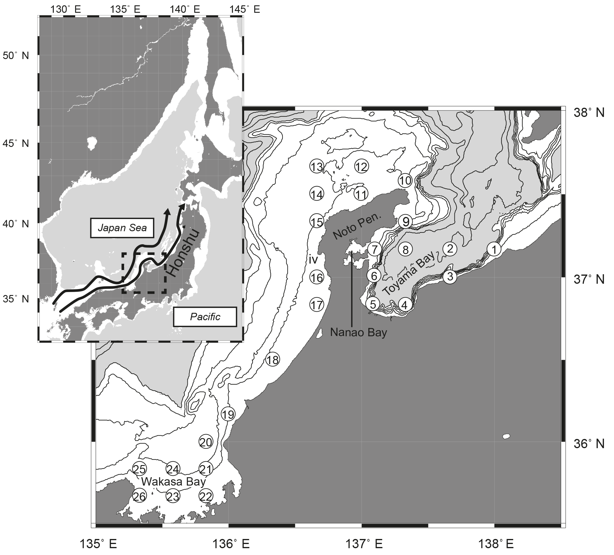
Figure 1Distribution of sampling stations (numbers in open circles) along the Japanese coast of the Japan Sea. Contours indicate bottom depth at 100 m intervals to 500 m depth (white areas), and 500 m intervals thereafter (gray areas). The superimposed map shows the location of the study area in the Japan Sea, and arrows in the map show the Tsushima Warm Current according to Hase et al. (1999).
At each station, vertical profiles of temperature and salinity were recorded using an STD (salinity–temperature–depth) sensor (Alec Electronics, AST1000) during the Mizunagi cruises (until 2011) or a CTD (conductivity–temperature–depth) sensor (Seabird, SBE9plus) during the Mizuho-maru cruises (after 2012) from the surface to 150 m depth or 5 m above the bottom (but only 5 m pitch during 1999–2001). Temperature and salinity were discarded at two stations, stn. 4 in 1999 and stn. 14 in 2001, due to mechanical malfunction. As the temperature- and density-based definition of the depth of the mixed layer (Zm) is similar in the Japan Sea (Lim et al., 2012), Zm was defined as that at which the temperature is 0.5 ∘C below the temperature at 5 m depth, as modified from Levitus (1982).
Zooplankton were collected with vertical hauls of a long Norpac net (Nytal 52GG, 335 µm mesh, 0.45 m mouth diameter, Rigo) from 150 m depth or 5 m above the bottom to the surface. A Rigo flowmeter, calibrated before and after every cruise, was installed at the mouth of the net for estimation of filtered water volume. Since macrozooplankton generally show diel vertical migration, our observations were mainly conducted during daytime (from 6 to 19 h); with observations at six stations conducted after 19 h (Fig. 2b). Zooplankton samples were fixed soon after sampling with neutral formalin and stored at room temperature until morphological identification. In the laboratory, all large zooplankton (approximately > 2 mm) in a sample were picked up for identification, and then the remaining sample was divided into subsamples using a Folsom or Motoda plankton splitter or a wide-bore pipette. The subsamples were split as the copepods in each subsample were 150–200 individuals. Individuals were identified to species level based on Chihara and Murano (1997), and then the density of each zooplankton species was calculated (individuals per cubic meter, inds. m−3). In the case of copepods, only adults and C4 and C5 stages of copepodites were identified and counted. The subsamples were observed until the number of the most dominant copepod species exceeded 150 inds; 2 % of a sample were observed on average. The people who identified zooplankton species were same in our study period; this means constant levels of accuracy and precision in the zooplankton community identification were maintained. In 1999, samples were lost at stns. 10 and 13 due to decay.

Figure 2Spatial variations of (a) day of May; (b) time of day; (c) mean temperature of the water column (mean T); (d) salinity at 5 m depth (SSS); (e) temperature at 5 m depth (SST); (f) maximum salinity of the water column; (g) mixed layer depth (Zm); and (h) sea surface chlorophyll a concentration in May (SSChl a). The x axis indicates the station number. The plots show the median (horizontal lines within boxes), upper and lower quartiles (boxes), quartile deviation (bars), and outliers (circles).
2.2 Other hydrographic data
Daily sea surface absolute height (SSH) and absolute current velocity data were derived from merged satellite data provided by AVISO (http://aviso.altimetry.fr, last access: 1 June 2018) between 1999 and 2013 at a spatial resolution of 0.25∘ × 0.25∘.
No primary productivity parameters were measured during the Mizunagi cruises, and thus the monthly composite sea surface chlorophyll a (SSChl a) concentration was derived from GlobColour (http://hermes.acri.fr, last access: 1 June 2018), which uses merged sensor GSM (Garver–Siegel–Maritorena) products (Maritorena et al., 2010). The spatial resolution was 4 × 4 km, and the SSChl a concentration of a station was taken from the nearest-neighbor data point. The validation of daily SSChl a data in Toyama Bay has already been reported by Terauchi et al. (2014). The monthly composite data were chosen in our study to avoid having many data blanks.
Sea surface net heat flux (Qnet) was calculated by using data sets derived from the Japanese 55-year Reanalysis (JRA-55, http://jra.kishou.go.jp, last access: 1 June 2018), with a spatial resolution of approximately 0.5∘ × 0.5∘, and the temporal resolution was set as monthly in this study. Qnet was calculated using the following equation shown in the atlas of JRA-55 (http://ds.data.jma.go.jp/gmd/jra/atlas/en/index.html, last access: 1 June 2018);
In Eq. (1), Qdswr, Qdlwr, Quswr, Qulwr, Qlh, and Qsh represent downward shortwave radiation, downward longwave radiation, upward shortwave radiation, upward longwave radiation, latent heat flux, and sensible heat flux, respectively.
2.3 Statistical analysis
Hypothesis-driven canonical analysis was used to evaluate the zooplankton community and environmental influences on zooplankton community structure. The calculation was performed using R software (R Core Team, 2017). Canonical analysis is a combination of an ordination technique and regression analysis. Four approaches are applicable for reduced space ordination applied to zooplankton community structures: principal component analysis (PCA), correspondence analysis (CA), nonmetric multidimensional scaling (NMDS), and principal coordinate analysis (PCoA) (Ramette, 2007). PCA is most frequently used in exploratory analysis as well as for clustering (Ramette, 2007); however, there are some prerequisites: the data must be quantitative, have a small number of blanks (null data), and show multivariate normality (Legendre and Legendre, 2012). Our plankton community data were quantitative, and to avoid too many blanks (null data), populations were excluded from the analysis if they met any of the following rules: (1) never above 5 % of total numerical abundance in all samples; (2) absent at all 26 stations in one-third of the observation periods (5 years); and (3) not able to be identified to species level. However, Mardia's test in the multivariate normality (MVN) package (Korkmaz et al., 2014) demonstrated our community data were not multivariate normal (p < 0.001); therefore, PCoA was applied. The NMDS approach was also appropriate, but for comparison of the environmental parameters using canonical analysis, PCoA was considered to be superior.
Table 1Environmental parameters and associated variance inflation factor (VIF) values.
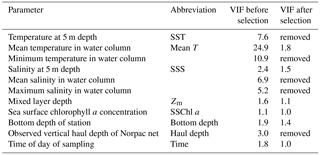
For hypothesis-driven canonical analysis, we used distance-based redundancy analysis (db-RDA), with PCoA as the ordination technique (Ramette, 2007). Before the db-RDA, multicollinearity in the environmental factors was checked using the variance inflation factor (VIF). Usually, VIF values of 10 are taken as the threshold of multicollinearity (Borcard et al., 2011), but in this study, the threshold was applied more strictly: only parameters with a VIF < 3 were selected. The environmental parameters are listed in Table 1: temperature at 5 m depth (SST), water column mean temperature (from 0 to 150 m or bottom 5 m depth; mean T), minimum temperature (corresponding to temperature at 150 m or bottom 5 m depth), salinity at 5 m depth (SSS), water column mean salinity, maximum salinity,Zm, and SSChl a as the water quality; bottom depth as the geographical information; and haul depth and observation time of day as the station information. The year is a possible explanatory parameter, but as this study focused on spatial variations, the effect of year was removed using partial db-RDA as a categorical variable. Initially, the VIF values of mean T, SST, minimum temperature, mean salinity, max salinity, and haul depth were > 3 (Table 1); this means they exhibited similar spatiotemporal variations. Since temperature is important for the zooplankton physiology, one of three temperature parameters should be kept in analysis at least. When we removed the parameters with highest VIF values until VIF values of the remaining parameters were < 3, all three temperature parameters were removed. Therefore, we kept the mean T as the representative parameters of the others (SST, minimum temperature, mean salinity, max salinity, and haul depth) for the db-RDA, and discarded the other high VIF parameters. As a result, VIF values of the remaining parameters were < 2.0 (Table 1). We then checked that the parameters significantly explained the zooplankton community variations based on AIC (Akaike information criterion) (Blanchet et al., 2008); as a result, time of sampling was excluded from the analysis. Therefore, the remaining environmental parameters comprised mean T, SSS, Zm, and bottom depth.
After the remaining environmental factors were standardized to Z scores, scaling to a mean of 0 and standard deviation of 1, db-RDA (including preprocessing) was conducted using the VEGAN package (Oksanen et al., 2007), and detailed codes were based on Borcard et al. (2011). The distance between species was calculated by the Bray method. The db-RDA outputs scores for environmental parameters, stations, and species. The contribution of environmental factors to the axes was evaluated in terms of the coefficient values of the explanatory equations. Aside from this main analysis, we supplementarily conducted another partial db-RDA with environmental parameters SST, max salinity, Zm, and bottom depth; the only coefficient values of the supplemental analysis were shown in the discussion session of this study.
3.1 Environmental conditions
Mean T varied from 10.96 to 17.28 ∘C and showed a decreasing tendency from west to east along the coastline (Fig. 2c). The 15-year mean T was 16∘ C at stn. 26 and clearly lower at < 12 ∘C at stns. 1–2, and the west–east decrease in mean T was reproduced in every year. The spatial trends in minimum temperature, SST, mean salinity, and max salinity were similar to mean T (data not shown), as shown by the high VIF values (Table 1). SSS ranged from 29.0 to 34.58; lower values (< 33) were often observed at stns. 1–9, which are located in Toyama Bay where large rivers discharge (Fig. 2d). Zm ranged from 5 to 118 m (Fig. 2e) and did not show significant spatial variation (ANOVA, p=0.78). The greatest Zm was observed in 2007, which is shown as outliers in Fig. 2e. Monthly high SSChl a concentration (> 2 mg m−3) was only observed at stations in Wakasa and Toyama bays (Fig. 2f), and mainly remained 0.2–0.5 mg m−3.
SSH was lower in Toyama Bay than in any of the other areas, with an area of high SSH extending from the Noto Peninsula to the northeast, and current velocity was < 15 cm s−1 (Fig. 3). The CBTWC was explicitly observed from Wakasa Bay to the Noto Peninsula; however, it was ambiguous in Toyama Bay. The monthly mean Qnet changed from negative to positive in April (Fig. 4a), and the mean Qnet in March–May showed no spatial differences (Fig. 4b).
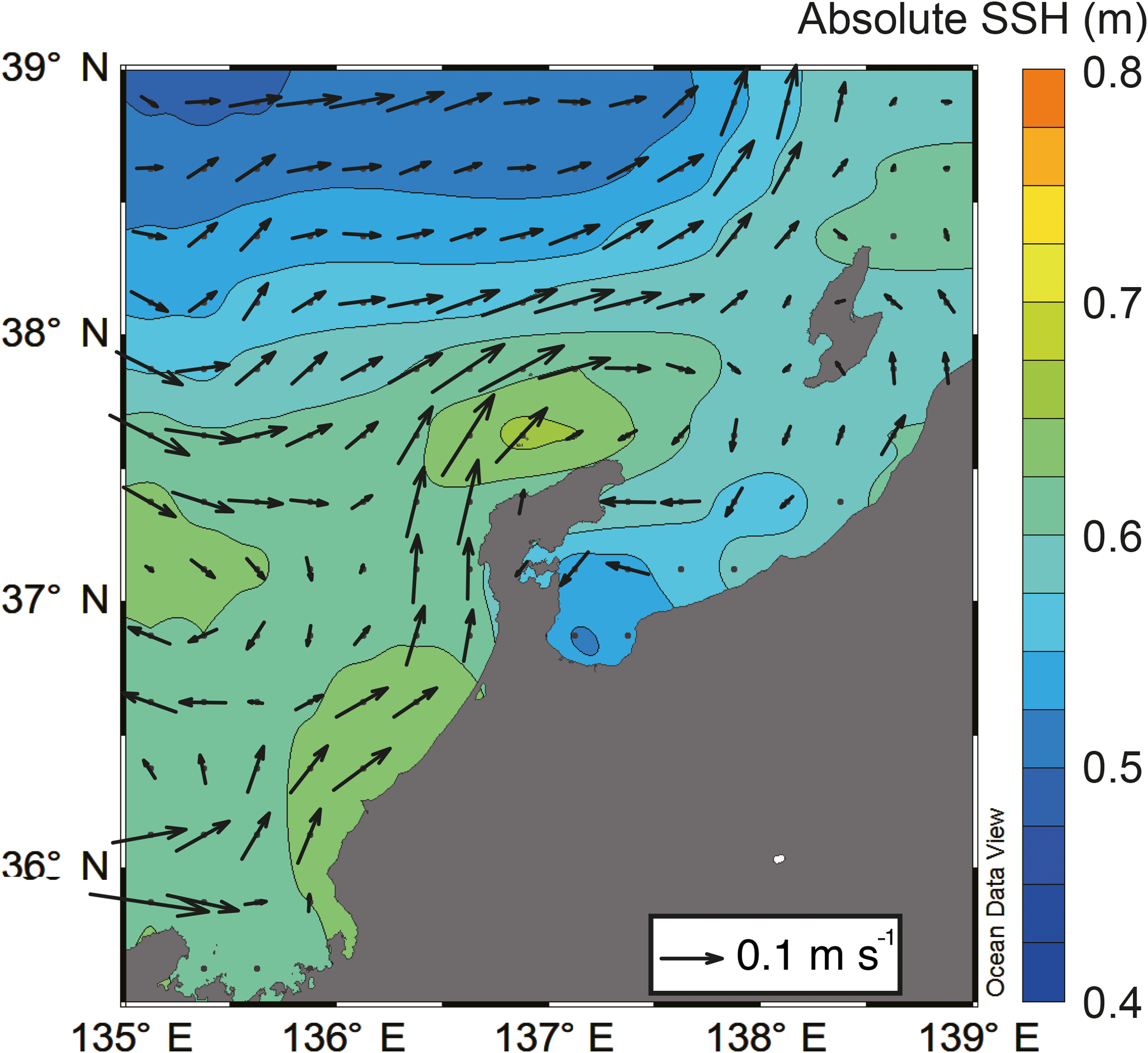
Figure 3Horizontal distribution of mean absolute sea surface height (colors) and mean current velocity (arrows) in May estimated by AVISO.
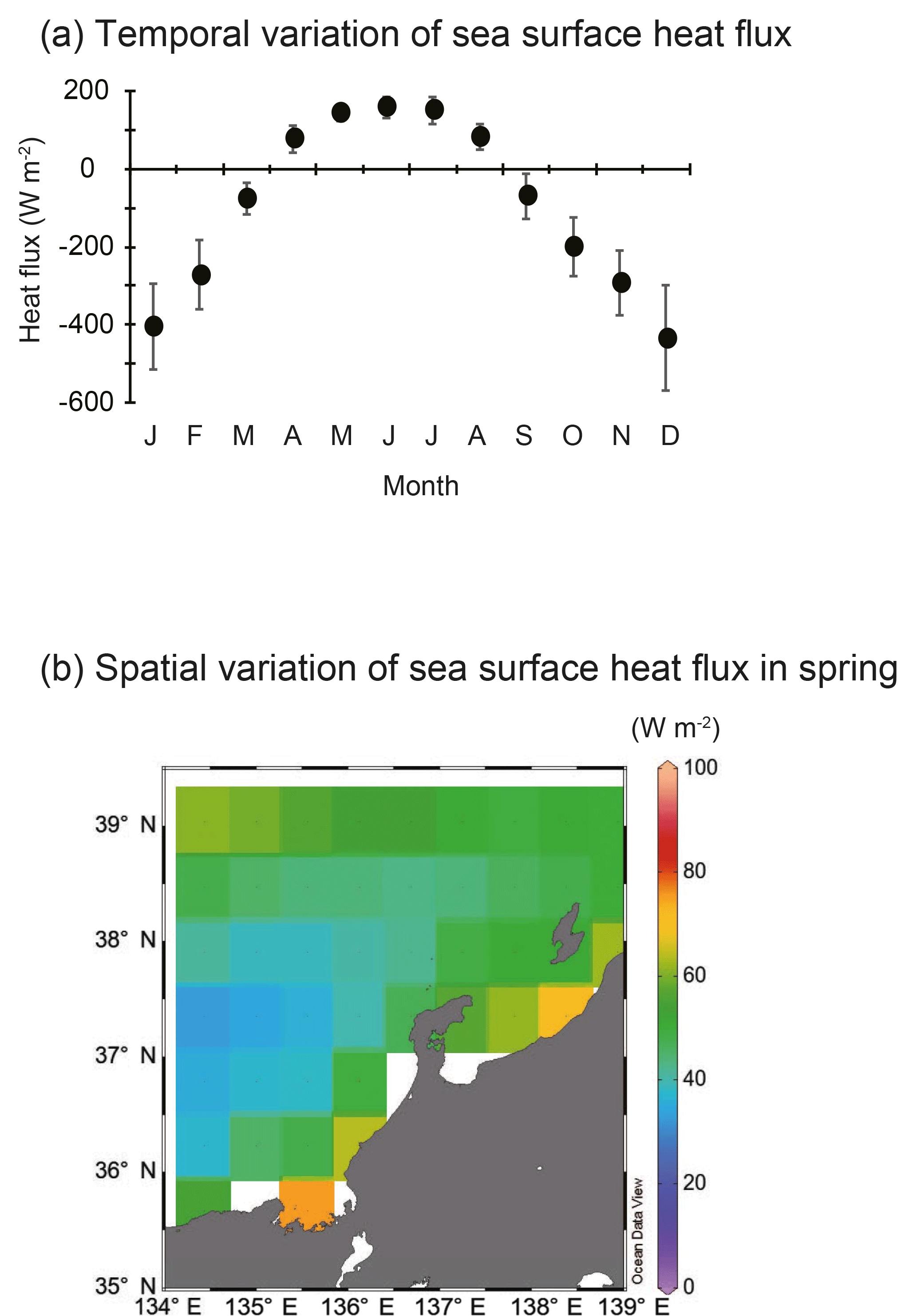
Figure 4Temporal and spatial variations in sea surface heat flux. (a) Annual variations in sea surface heat flux (W m−2) between 2000 and 2013 in the area of 134–139∘ E and 35– N. Vertical bars denote 1 standard deviation. (b) Spatial variation of sea surface heat flux (W m−2) during spring (March–May) from 2000 to 2013. Blank areas were excluded because they were ascribed as landmass in JRA-55.
3.2 Zooplankton abundance and community structures
Overall, 78 species were identified from 388 samples. Some specimens were limitedly identified to genus level, since key parts for identification were destroyed. The top 10 dominant species from an average of all stations contained seven copepods (Corycaeus affinis, Oithona atlantica, Calanus sinicus, Ctenocalanus vanus, Paracalanus parvus s.l., Oithona plumifera, and Pseudocalanus newmani), plus one each of Appendicularia (Oikopleura longicauda), Euphausiacea (Euphasia pacifica), and Cladocera (Evadne nordmanni). Spatially, the dominant species differed in the west and east: in the west, C. affinis and C. sinicus were the first and second most dominant species on average, while O. atlantica was most dominant in the east, apart from stn. 7 (Fig. 5a). C. affinis and E. nordmanni showed the largest temporal variation (Fig. 5b): C. affinis was abundant in 2006 and 2010, and E. nordmanni was dominant in 2004.
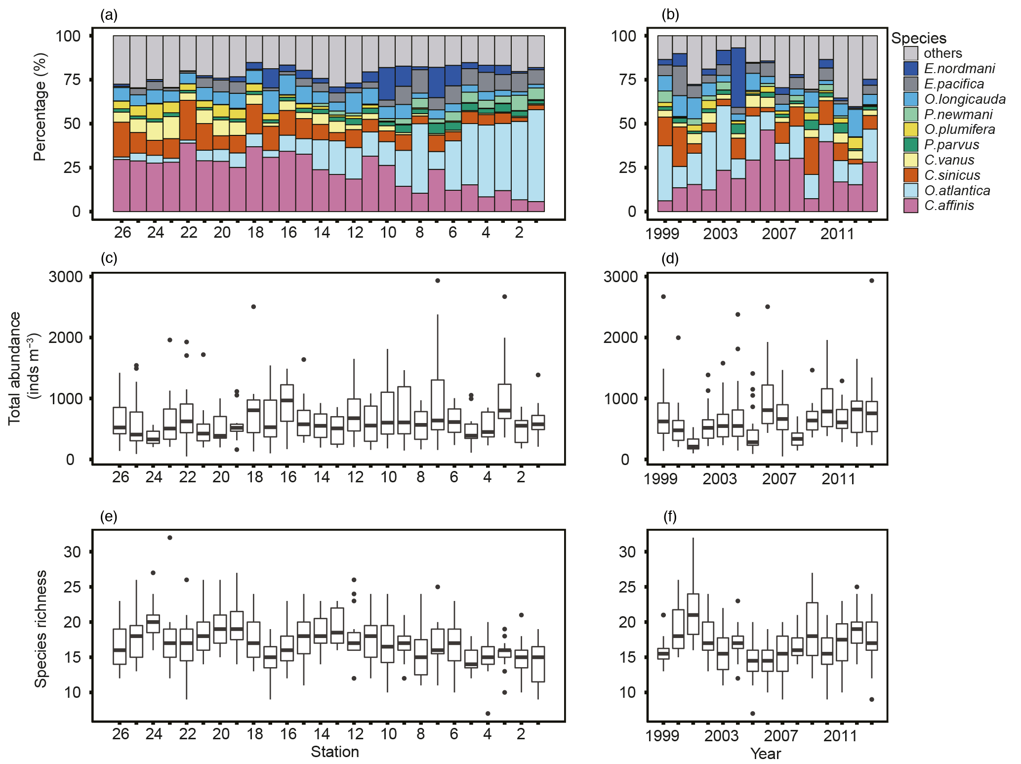
Figure 5Spatial and yearly variations of contributions of top 10 most abundant species (a, b), total zooplankton abundance (c, d), and species richness (e, f). The total zooplankton abundance plots show the median (horizontal lines within boxes), upper and lower quartiles (boxes), quartile deviation (bars), and outliers (circles).
Total abundance largely varied from 48 to 2933 inds. m−3 (mean ± SD: 649 ± 418 inds. m−3); there was no clear west–east tendency in abundance (Fig. 5c). The highest mean abundances were recorded at stns. 3 and 7 in Toyama Bay, with 1009 ± 613 and 975 ± 800 inds. m−3, respectively, and stn. 24 in Wakasa Bay recorded the lowest with 361 ± 125 inds. m−3. There was no trend in the temporal variation of total abundance (Fig. 5d). The species richness (S), the number of appeared species at a station, ranged 7 to 32: the lower and upper quartile values were 15 and 19, respectively (Fig. 5e). The interannual variation of S had a peak in 2001 and remained high from 2009 to 2013 (Fig. 5f).
3.3 Multivariate analysis
After preprocessing, 25 zooplankton species remained for multivariate analysis. In addition to the top 10 species, there were two Chaetognatha (Sagitta minima and S. nagae), two Cladocera (Podon leuckarti and Penilia avirostris), nine copepods (Metridia pacifica, Acartia omorii, Candacia bipinnata, Centropages bradyi, Mesocalanus tenuicornis, Neocalanus plumchrus, Clausocalanus pergens, Oncaea mediterranea, and Oncaea venusta), one Hyperiidea (Themisto japonica), and one Appendicularia (Fritillaria pellucida). The 25 species accounted for 94 % of total abundance on average, although only ∼ 70 % at some stations. At the latter stations, Oithona longispina and/or Oithona spp. were highly abundant after 2010.
The db-RDA results for total, conditioned, and constrained inertia were 112.63, 18.64, and 17.08, respectively. Three axes of zooplankton community structure variation were significantly explained in the db-RDA (ANOVA, p < 0.05): the eigenvalues of the first, second, and third axes (RD1–3, respectively) explained 89.9, 4.9, and 2.5 % of zooplankton community structure variability, respectively.
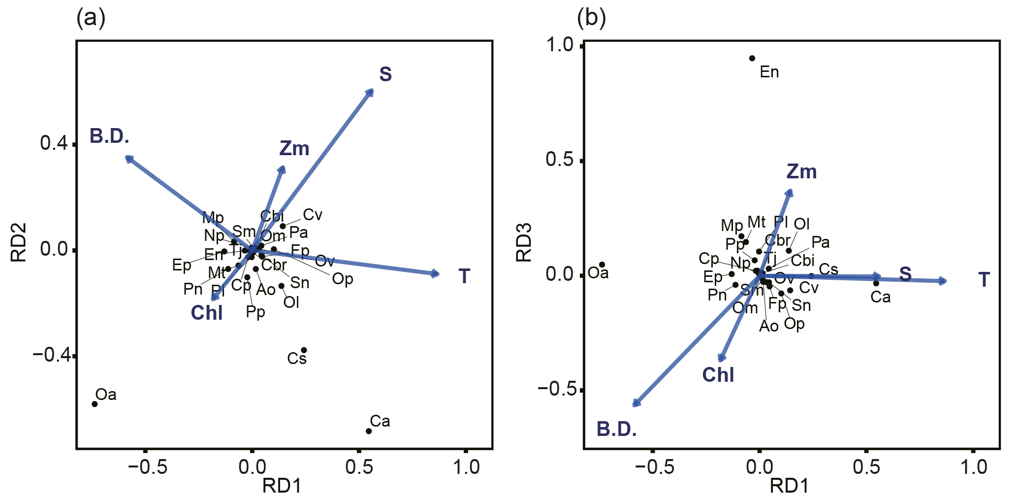
Figure 6Relationship between environmental parameters (arrows) and zooplankton species (crosses) in the db-RDA diagram: (a) combination of RD1 and RD2, and (b) combination of RD1 and RD2. The abbreviations T, S, Chl, Zm, and B.D. adjacent to arrows represent mean temperature of water column (mean T), salinity at 5 m depth (SSS), sea surface chlorophyll a (SSChl a), mixed layer depth (Zm), and bottom depth of station, respectively. The 25 zooplankton spices were represented by their initials.
The relationship between species and environmental parameters is shown in Fig. 6, after scaling the site score using biplot diagrams (Fig. 6); the site score was removed from Fig. 6 since their plot was invisible due to their numbers (n=388). First, on the combination of RD1 and RD2, the absolute values of mean T were large in RD1 but small in RD2 (Fig. 6a). The absolute values of SSS in RD1 and RD2 were the same level; that in RD2 was largest among the five parameters. Bottom depth was the parameter for which RD1 was largely negative. Of the zooplankton species, C. affinis and O. atlantica plotted in the second and third quadrants: the RD1 values were the opposite of each other, but both of those RD2 values were plotted negative. C. vanus was plotted in the first quadrant, C. sinicus and O. longicauda were plotted in the second quadrant, and the other species were located near the origin. Second, in the combination of RD1 and RD3, E. nordmanni was plotted far away from the axis of RD3 = 0 (Fig. 6b). Bottom depth and SSChl a were largely negative, and Zm was positive on RD3.
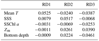
Mean T had the highest coefficient on RD1, 0.0525 (Table 2), and those of the other parameters were at least one-sixth that of mean T; the second highest was 0.0079 for SSS. On RD2, SSS had the largest absolute coefficient value (0.0517), and the absolute values of the other three parameters (mean T, Zm, and bottom depth) were the same level (0.022–0.026). On RD3, bottom depth was largest (−0.046), and Zm and mean T were next (−0.034).
Table 2Coefficients for environmental parameters calculated using db-RDA.
In terms of spatial features, RD1 showed a west–east trend: it was relatively low from stns. 1 to 8 (except at stn. 7), corresponding to Toyama Bay, and relatively high from stns. 16 to 26, corresponding to the western part of Noto Peninsula to Wakasa Bay (Fig. 7a). RD1 values in Toyama Bay (stns. 1–8, except 7) were significantly different from those in the northern part of the Noto Peninsula to Wakasa Bay (stns. 9–26) (Tukey's test, p < 0.001). The RD1 of stn. 7 was significantly different from the other Toyama Bay stations, and similar to stns. 9–15, corresponding to the northern part of Noto Peninsula. The RD2–3 did not show west–east trends, and showed high or low values in stns. 2 and 8 compared to the other stations (Fig. 7b, c).
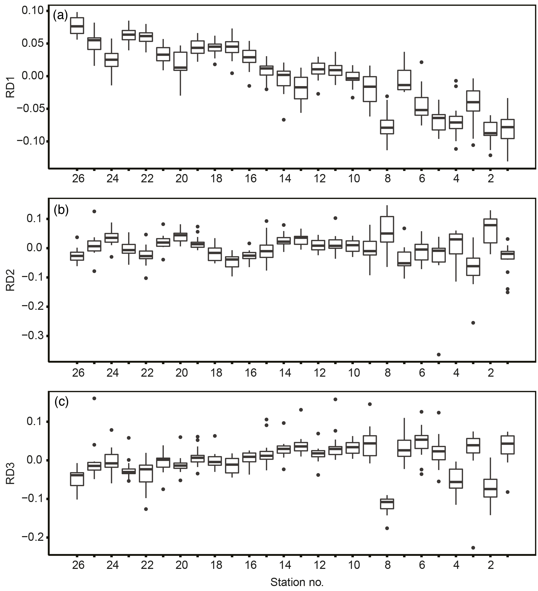
Figure 7Spatial variation of station db-RDA scores: (a) RD1, (b) RD2, and (c) RD3. Plots show the median (horizontal lines within boxes), upper and lower quartiles (boxes), quartile deviation (bars), and outliers (circles).
In our study, zooplankton abundance differed between the stations (Fig. 5); however, there was no clear west–east gradient. This finding is similar to that of a previous study by Hirota and Hasegawa (1999), which found that zooplankton abundance (wet weight) is homogenous along the Japanese coast at a spatial resolution of 1∘ × 1∘.
4.1 Interpretation of multivariate analysis
Since the equations with coefficient values calculated from db-RDA are only “hypotheses”, the db-RDA results need to be interpreted in terms of the species score. Before the analysis, some environmental parameters were dropped based on the VIF and AIC values. The sampling time was removed from the explanatory variables based on the AIC values, but some previous studies show the diel migration of zooplankton in Toyama Bay: the wet weight of zooplankton in the 0–150 m range is high in the nighttime (Hirota and Hasegawa, 1999), and the evident diel vertical migrations in spring are reported on E. pacifica (Iguchi, 1995) and M. pacifica (Takahashi and Hirakawa, 2001). Our consideration for rejecting the sampling time from the explained values was that the sampling was mostly done in the daytime (Fig. 2b), and the bottom depth is shallow in the western part of our sampling site (Fig. 1). On the other hand, our results show the daytime zooplankton community structure: the variation of nighttime may be different.
From the db-RDA with mean T, SSS, Zm, SSChl a, and bottom depth, variations in zooplankton community structure were mainly distributed along three axes, and most of the variance was explained by RD1. The coefficients (Table 2) show that the variation in RD1 is largely controlled by mean T. Zooplankton species that recorded positive (C. affinis, C. sinicus, C. vanus, and O. longicauda) and negative (O. atlantica, E. pacifica, and P. newmani) scores for RD1 (Fig. 6) are classified in the Japan Sea as warm- and cold-water species, respectively (Iguchi and Tsujimoto, 1997; Iguchi et al., 1999; Chiba and Saino, 2003). Therefore, this axis is interpreted as explaining spatial differences due to water temperature, and the equations on RD1 are considered to describe the zooplankton variation well.
Although RD2 and RD3 only show a minor contribution to the spatial variation of zooplankton community structure, we attempted to interpret the data. RD2, which explained 4.9 % of variation, is highly explained by SSS (Table 2), which is negatively related to C. affinis and O. atlantica (Fig. 6b). However, we cannot reasonably explain this axis. The low SSS indicated the supply of river discharge, and river discharged water contains a large amount of phytoplankton (Terauchi et al., 2014), while coefficient of SSChl a was low in this axis. Since O. atlantica is a suspension feeder (herbivorous), it was possible to explain reasonably that low SSS increases O. atlantica abundance. However, C. affinis is carnivorous, and thus the eutrophication did not directly have an influence on the population.
RD3, which explains 2.5 % of total variation, is positively affected by Zm and negatively affected by bottom depth and mean T (Table 2), and E. nordmanni was recorded positive. These mean that deep mixing with low temperature and shallow bottom depth increase the abundance of E. nordmanni. Abundance of E. nordmanni is increased in the cold season when SST is < 20 ∘C in Toyama Bay but not observed before February (Onbé and Ikeda, 1995). The resting eggs of E. nordmanni which only sink to the shallow sea bottom will hatch (Onbé, 1985); the shallow bottom depth is important for its reproduction, and thus the abundance was considered to be high in the shallow bottom areas. Therefore, we considered that the equation of this axis shows the spatial variation of E. nordmanni abundance following its life cycle and physiology.
4.2 Influence of the CBTWC
RD1 was the only axis that showed differences between the stations and expressed the main feature (89.9 %) of spatial variation in the zooplankton community structure in our investigation area. The axis showed greater spatial variation (Fig. 7). RD1 was interpreted as representing the dominance of warm- and cold-water species in Wakasa and Toyama bays, respectively, which is similar to the findings of previous studies at the same sites (Iguchi and Tsujimoto, 1997; Iguchi et al., 1999). Therefore, this feature is considered highly reproducible with temperature variation in our investigated area in May.
However, the environmental differences between Toyama Bay and the other areas were not limited to temperature: the bottom depth with the submarine canyon was deep (Fig. 1), and SSS was low (Fig. 2d) because of the river input in Toyama Bay. These affect the zooplankton community as well as temperature. For example, the subsurface canyon is the habitat of zooplankton, and the zooplankton migrate to shallow layer (Herman et al., 1991), and cold-water species are dominant in the deep layer of the Toyama Bay (Takahashi and Hirakawa, 2001). For example, in the Mediterranean Sea, the river input changes the amount of phytoplankton, which in turn affects the amount of zooplankton (Espinasse et al., 2014). In our study area, river input to the Toyama Bay raises the sea surface chlorophyll a concentration (Terauchi et al., 2014), and thus these should be considered as the factors which were affected by the difference in the zooplankton community structure in Toyama Bay and other areas.
In other studies, it was shown that the deep layer is the habitat of zooplankton which migrate to shallower depth (e.g., Herman et al., 1991), and thus the bottom depth should be important for the migratory zooplankton. In the RD1, however, the coefficient value of bottom depth was very low (Table 2). This indicated that the bottom depth did not directly contribute to the zooplankton community structure. We considered the sampling time to be one of the reasons why the bottom depth has only a minor contribution in RD1: our sampling time was mainly daytime, and thus zooplankton such as E. pacifica, M. pacifica, and T. japonica, which are present in the deep layer in daytime and migrate to surface layer in nighttime (Ikeda et al., 1992; Iguchi, 1995; Takahashi and Hirakawa, 2001), were limited to be collected.
Pollution (eutrophication) and river discharge are sometimes considered to determine community structure in areas such as the Mediterranean (Siokou-Frangou et al., 1998), the Brazilian coast (Valentin and Monteiroribas, 1993), the coastal area of Taiwan (Chou et al., 2012), and coast of North America (Pepin et al., 2015); however, the low coefficient values of SSS and SSChl a in our db-RDA results show that eutrophication is not the principal determinant of zooplankton community structure in the Japan Sea. The cause of this is not clear in this study, but we consider two possible explanations: (1) the observation period was at the end of the spring bloom, and local upwelling along the shelf edge in our study area occurs during summer (Nakada and Hirose, 2009); thus, the area was not oligotrophic, and the food condition was not important; (2) less-saline water was only present at the surface (< 10 m depth), and most of the water column was not affected by the less-saline eutrophic water. However, difference in the feeding habits of the dominant zooplankton (i.e., carnivore C. affinis and herbivore O. atlantica) may depend on the difference of primary productivity among areas. In addition, Oithona prefer the stratified condition for feeding (Saiz et al., 2003); less-saline surface water possibly contributes to the stratification, and thus O. atlantica may increase in Toyama Bay.
Spatial variations of zooplankton shown in RD1 are largely explained by mean T. Factors controlling temperature are likely to be responsible for spatial variations in zooplankton community structure. Three factors potentially control the spatial variation of water temperature: (1) Qnet, net heat flux; (2) mixing with cold deep-sea water; and (3) heat supply by horizontal advection. Qnet controls stratification of water column and the timing of spring phytoplankton bloom (Taylor and Ferrari, 2011), but increase of zooplankton abundance is not associated with change of Qnet in the English Channel (Smyth et al., 2014). The timing of the change from negative to positive Qnet (Fig. 4a) coincides with that of sea surface temperature increase in Toyama Bay. Additionally, no spatial differences in the Qnet were observed in the study area (Fig. 4b), which is consistent with previous studies (Hirose et al., 1996; Na et al., 1999). This suggests that Qnet is not the controlling factor on spatial variations in temperature except in Toyama Bay, and indicates that other heat supply processes may be more important. The second potential factor, mixing between cold deep-sea water, initially seems to have greater potential as the bottom depth of stations in Toyama Bay was deeper than elsewhere. Bottom depth was a remaining significant explanatory factor, but its coefficient value was low on RD1 (Table 2). Therefore, mixing between cold deep-sea water is not considered to be the main factor controlling the spatial variation of temperature, although its influence cannot be completely discounted. We consider that the zooplankton abundance and community structure is generally not explained by “on-site” (in situ) environmental variations: large ocean systems can also influence the local zooplankton community variations, which is also observed in European seas (Frid and Huliselan, 1996; Reid et al., 2003; Smyth et al., 2014).
The final potential control on sea surface temperature is horizontal advection by the CBTWC. Previous studies have indicated that the heat content of the Japan Sea is largely affected by horizontal advection associated with the TWC, particularly from April to October (Hirose et al., 1996). In our study, SSH values suggest that the path of the CBTWC was parallel to the mouth of Toyama Bay (Fig. 3), and indicates that the intrusion of the CBTWC is weak and rare in Toyama Bay. Weak and rare intrusion of the CBTWC in Toyama Bay is supported by previous studies (Hase et al., 1999; Nakada et al., 2002) and is attributed to the break of continental shelf in Toyama Bay (Nakada et al., 2002; Igeta et al., 2017). The CBTWC is trapped on the continental shelf and flows along the isodepth from the Tsushima Strait to the Noto Peninsula (Kawabe, 1982); breaks in the continental shelf at Noto Peninsula can potentially alter the direction of the current. The spatial variation of site scores on RD1 corresponds to the bottom topography; higher scores were observed on the continental shelf (stns. 7 and 9), and there were lower scores in the downstream reach of the submarine canyon.
Nakada et al. (2002) and Igeta et al. (2017) evaluated the effect of Toyama Bay topography (the submarine canyon, Fig. 1) on the CBTWC using a simple two-layer numerical model. They showed that breaks in the continental shelf induce cyclonic eddies at the edge of the Noto Peninsula, which were sometimes transported to the north, while if the continental shelf is unbroken, the coastal current spreads widely into Toyama Bay. In contrast, the continental shelf is wider at Wakasa Bay (Fig. 1), and water exchange is active during winter (Itoh et al., 2016); here, and along the western part of Noto Peninsula, the zooplankton community structure on RD1 was homogenous.
The importance of ocean currents for zooplankton community structure has also been demonstrated in coastal areas facing the open ocean, such as the Kuroshio off Japan (Sogawa et al., 2017), and on the Pacific and Atlantic coasts of North America (Mackas et al., 1991; Keister et al., 2011; Pepin et al., 2011; Pepin et al., 2015). In our study, the response of zooplankton to temperature was focused after VIF selection, but the horizontal advection of zooplankton by the CBTWC is also relevant; the importance of the original zooplankton community structure has been demonstrated in a study of eddies associated with the Leeuwin Current off Australia (Strzelecki et al., 2007). When the other db-RDA was done with max salinity and SST as the explanatory parameters instead of mean T and SSS, the coefficients of SST and maximum salinity were 0.0392 and 0.0192, respectively. The SST variation was considered as the results of the CBTWC, water temperature in winter and Qnet, while the maximum salinity was one of the indices of CBTWC transport, because the maximum of salinity of the TWC is increased from spring to summer at the Tsushima Strait (Morimoto et al., 2009). Therefore, we considered that the contribution of CBTWC was at least one-third of RD1 variation. Hence, as it was difficult to completely separate the effects of temperature and zooplankton transportation, the CBTWC can be assumed to be an important control on zooplankton community structure.
The spatial variation in Toyama Bay and other areas has been discussed, but differences were also observed between the northern and western parts of the Noto Peninsula, which are downstream and upstream of the CBTWC, respectively (Fig. 4). This difference may result from differences in the original water masses and zooplankton communities. Since the velocity of the CBTWC is ∼ 10 cm s−1 and rarely > 30 cm s−1 (Hase et al., 1999; Igeta et al., 2011; Fukudome et al., 2016), it takes ∼ 10 days for a water mass to travel 100 km. Wakasa Bay is ∼ 500 km from the Tsushima Strait, so it is possible for water that is present in the Tsushima Strait in March to reach Wakasa Bay and the western part of Noto Peninsula in May; however, it would not yet reach the northern part of Noto Peninsula, which is ∼ 700 km from the Tsushima Strait. Near the Tsushima Strait, dominant copepods in the upstream CBTWC include the warm-water species C. sinicus, P. parvus, and C. vanus, even in March (Hirakawa et al., 1995); cold-water species are present and dominant in the Japan Sea during winter (Chiba and Saino, 2003).
The dominance of warm-water zooplankton can be treated as the key indicator of the CBTWC. Zooplankton communities have been treated as water mass indicators in other areas (Russell, 1935). Rapid changes in zooplankton community in response to oceanic currents have been identified in areas such as the Kuroshio coast and Mediterranean (Raybaud et al., 2008; Sogawa et al., 2017), which were different in our study site; similar zooplankton community was observed every year in May. In addition, the dominance of the herbivorous O. atlantica in Toyama Bay suggests its food web structure differs from the other areas, which are dominated by the carnivorous C. affinis (Ohtsuka and Nishida, 1997); the effect of bottom topography on the path of the CBTWC creates a heterogenic ecosystem along the Japanese coast in the Japan Sea. Previously, it was known that submarine canyons have impacts on the pelagic ecosystem via local upwelling (Fernandez-Arcaya et al., 2017). In Toyama Bay, there is cyclonic circulation when the CBTWC intrudes (Igeta et al., 2017), which produces downwelling. Therefore, our results show that changes in the path of the current induced by the submarine canyon promote ecosystem heterogeneity and the rich spatial biodiversity along the coast of Japan.
We investigated zooplankton community structure over a 15-year period along the Japanese coast of the Japan Sea, with the continental shelf and a submarine canyon. Distance-based RDA indicated that zooplankton community structure is largely influenced by water temperature of the CBTWC. Warm-water zooplankton were dominant in the path of the CBTWC and along the Japanese coast, and cold-water zooplankton were dominant in Toyama Bay where intrusion of the CBTWC is prevented by a submarine canyon. Therefore, dominance of warm-water species can be used as an index of the CBTWC along the Japanese coast of the Japan Sea. Even though our study area was close to the coast, the effect of land is not dominant, and biological productivity is mainly controlled by the ocean. Surface waters in the Japan Sea have been affected by global warming and east Asian industrial development for half a century (Belkin, 2009; Kodama et al., 2016). Our study indicates that water temperature largely determines the zooplankton community; therefore, an elevation in sea surface temperature is likely to change zooplankton community structure. Continuous monitoring in our study site helps the effects of global warming on biological productivity to be better understood.
The data sets are available in the Supplement.
The supplement related to this article is available online at: https://doi.org/10.5194/os-14-355-2018-supplement.
The authors declare that they have no conflict of interest.
We thank the captain, officers, and crew of the T/V Mizunagi of the Kyoto
Prefecture and R/V Mizuho-maru of the Japan Fisheries and Education
Research Agency cruise for their cooperation at sea. The altimeter
products were produced by Ssalto/Duacs and distributed by AVISO, with support
from CNES (http://www.aviso.altimetry.fr/duacs/, last access: 1 June 2018). The chlorophyll a was obtained from GlobColour
project: GlobColour data (http://globcolour.info, last access: 1 June 2018) used in this study have been developed, validated,
and distributed by ACRI-ST, France. We deeply appreciate an anonymous
referee, and Sabine Schultes for their insightful comments in our discussion
paper. This study was financially supported by general research funds from
Japan Fisheries Research and Education Agency and the Fisheries Agency to
all, a research project of the Agriculture, Forestry and Fisheries Research
Council (Development of technologies for mitigation and adaptation to climate
change in agriculture, forestry and fisheries) to Taketoshi Kodama, Taku
Wagawa and Haruyuki Morimoto, and a JSPS grant (16K07831) to Taketoshi Kodama
and Taku Wagawa.
Edited by: Mario Hoppema
Reviewed by: Sabine Schultes and one anonymous referee
Beaugrand, G.: Monitoring pelagic ecosystems using plankton indicators, ICES J. Mar. Sci., 62, 333–338, https://doi.org/10.1016/j.icesjms.2005.01.002, 2005.
Belkin, I. M.: Rapid warming of large marine ecosystems, Prog. Oceanogr., 81, 207–213, https://doi.org/10.1016/j.pocean.2009.04.011, 2009.
Blanchet, F. G., Legendre, P., and Borcard, D.: Forward selection of explanatory variables, Ecology, 89, 2623–2632, https://doi.org/10.1890/07-0986.1, 2008.
Borcard, D., Gillet, F. O., and Legendre, P.: Numerical ecology with R, Springer, New York, 2011.
Chavez, F. P., Ryan, J., Lluch-Cota, S. E., and Niquen, C. M.: From anchovies to sardines and back: multidecadal change in the Pacific Ocean, Science, 299, 217–221, https://doi.org/10.1126/science.1075880, 2003.
Chiba, S. and Saino, T.: Variation in mesozooplankton community structure in the Japan/East Sea (1991–1999) with possible influence of the ENSO scale climatic variability, Prog. Oceanogr., 57, 317–339, https://doi.org/10.1016/S0079-6611(03)00104-6, 2003.
Chiba, S., Hirota, Y., Hasegawa, S., and Saino, T.: North-south contrasts in decadal scale variations in lower trophic-level ecosystems in the Japan Sea, Fish. Oceanogr., 14, 401–412, https://doi.org/10.1111/j.1365-2419.2005.00355.x, 2005.
Chihara, M. and Murano, M.: An illustrated guide to marine plankton in Japan, Tokai Univ., Tokyo, 1997.
Chou, W.-R., Fang, L.-S., Wang, W.-H., and Tew, K. S.: Environmental influence on coastal phytoplankton and zooplankton diversity: a multivariate statistical model analysis, Environ. Monit. Assess., 184, 5679–5688, https://doi.org/10.1007/s10661-011-2373-3, 2012.
Espinasse, B., Carlotti, F., Zhou, M., and Devenon, J. L.: Defining zooplankton habitats in the Gulf of Lion (NW Mediterranean Sea) using size structure and environmental conditions, Mar. Ecol. Prog. Ser., 506, 31–46, https://doi.org/10.3354/meps10803, 2014.
Fernandez-Arcaya, U., Ramirez-Llodra, E., Aguzzi, J., Allcock, A. L., Davies, J. S., Dissanayake, A., Harris, P., Howell, K., Huvenne, V. A. I., Macmillan-Lawler, M., Martín, J., Menot, L., Nizinski, M., Puig, P., Rowden, A. A., Sanchez, F., and Van den Beld, I. M. J.: Ecological role of submarine canyons and need for canyon conservation: A review, Frontiers in Marine Science, 4, 5, https://doi.org/10.3389/fmars.2017.00005, 2017.
Field, J. G., Clarke, K. R., and Warwick, R. M.: A practical strategy for analyzing multispecies distribution patterns, Mar. Ecol. Prog. Ser., 8, 37–52, https://doi.org/10.3354/Meps008037, 1982.
Frid, C. L. J. and Huliselan, N. V.: Far-field control of long-term changes in Northumberland (NW North Sea) coastal zooplankton, ICES J. Mar. Sci., 53, 972–977, 1996.
Fukudome, K., Igeta, Y., Senjyu, T., Okei, N., and Watanabe, T.: Spatiotemporal current variation of coastal-trapped waves west of the Noto Peninsula measured by using fishing boats, Cont. Shelf Res., 115, 1–13, https://doi.org/10.1016/j.csr.2015.12.013, 2016.
Goto, T.: Abundance and distribution of the eggs of the sardine, Sardinops melanostictus, in the Japan Sea during spring, 1979–1994, B. Jpn. Sea Reg. Fish. Res. Lab., 48, 51–60, 1998.
Goto, T.: Paralarval distribution of the ommastrephid squid Todarodes pacificus during fall in the southern Sea of Japan, and its implication for locating spawning grounds, B. Mar. Sci., 71, 299–312, 2002.
Hase, H., Yoon, J.-H., and Koterayama, W.: The current structure of the Tsushima Warm Current along the Japanese coast, J. Oceanogr., 55, 217–235, https://doi.org/10.1023/a:1007894030095, 1999.
Herman, A. W., Sameoto, D. D., Shunnian, C., Mitchell, M. R., Petrie, B., and Cochrane, N.: Sources of zooplankton on the Nova-Scotia shelf and their aggregations within deep-shelf basins, Cont. Shelf Res., 11, 211–238, 1991.
Hirakawa, K., Kawano, M., Nishihama, S., and Ueno, S.: Seasonal variability in abundance and composition of zooplankton in the vicinity of the Tsushima straits, southwestern Japan Sea, B. Jpn. Sea Nat. Fish. Res. Inst., 45, 25–38, 1995.
Hirose, N., Kim, C.-H., and Yoon, J.-H.: Heat budget in the Japan Sea, J. Oceanogr., 52, 553–574, https://doi.org/10.1007/bf02238321, 1996.
Hirose, N., Nishimura, K., and Yamamoto, M.: Observational evidence of a warm ocean current preceding a winter teleconnection pattern in the northwestern Pacific, Geophys. Res. Lett., 36, L09705, https://doi.org/10.1029/2009gl037448, 2009.
Hirota, Y. and Hasegawa, S.: The zooplankton biomass in the Sea of Japan, Fish. Oceanogr., 8, 274–283, https://doi.org/10.1046/j.1365-2419.1999.00116.x, 1999.
Hjort, J.: Fluctuations in the great fisheries of northern Europe viewed in the light of biological research, Rapp. P.-V. Reun. Cons. int. Explor. Mer., 20, 1–228, 1914.
Hooff, R. C. and Peterson, W. T.: Copepod biodiversity as an indicator of changes in ocean and climate conditions of the northern California current ecosystem, Limnol. Oceanogr., 51, 2607–2620, https://doi.org/10.4319/lo.2006.51.6.2607, 2006.
Igeta, Y., Watanabe, T., Yamada, H., Takayama, K., and Katoh, O.: Coastal currents caused by superposition of coastal-trapped waves and near-inertial oscillations observed near the Noto Peninsula, Japan, Cont. Shelf Res., 31, 1739–1749, https://doi.org/10.1016/j.csr.2011.07.014, 2011.
Igeta, Y., Yankovsky, A., Fukudome, K.-I., Ikeda, S., Okei, N., Ayukawa, K., Kaneda, A., and Watanabe, T.: Transition of the Tsushima Warm Current path observed over Toyama Trough, Japan, J. Phys. Oceanogr., 47, 2721–2739, https://doi.org/10.1175/jpo-d-17-0027.1, 2017.
Iguchi, N.: Spring diel migration of a euphausiid Euphausia pacifica in Toyama Bay, southern Japan Sea, B. Jpn. Sea Natl. Fish. Res. Inst., 45, 59–68, 1995.
Iguchi, N. and Kidokoro, H.: Horizontal distribution of Thetys vagina Tilesius (Tunicata, Thalicaea) in the Japan Sea during spring 2004, J. Plankton Res., 28, 537–541, https://doi.org/10.1093/plankt/fbi138, 2006.
Iguchi, N. and Tsujimoto, R.: Seasonal changes in the copepoda assemblage as food for larval Anchovy in Toayama Bay, southern Japan Sea, B. Jpn. Sea Nat. Fish. Res. Inst., 47, 79–94, 1997.
Iguchi, N., Wada, Y., and Hirakawa, K.: Seasonal changes in the copepoda assemblage as food for larval Anchovy in western Wakasa Bay, southern Japan Sea, B. Jpn. Sea Nat. Fish. Res. Inst., 49, 69–80, 1999.
Ikeda, T., Hirakawa, K., and Imamura, A.: Abundance, population structure and life cycle of a hyperiid amphipod Themisto japonica (Bovallius) in Toyama Bay, southern Japan Sea, Bull. Plankton Soc. Japan, 39, 1–16, 1992.
Isobe, A., Ando, M., Watanabe, T., Senjyu, T., Sugihara, S., and Manda, A.: Freshwater and temperature transports through the Tsushima-Korea Straits, J. Geophys. Res., 107, 2-1–2-20, https://doi.org/10.1029/2000jc000702, 2002.
Itoh, S., Kasai, A., Takeshige, A., Zenimoto, K., Kimura, S., Suzuki, K. W., Miyake, Y., Funahashi, T., Yamashita, Y., and Watanabe, Y.: Circulation and haline structure of a microtidal bay in the Sea of Japan influenced by the winter monsoon and the Tsushima Warm Current, J. Geophys. Res., 121, 6331–6350, https://doi.org/10.1002/2015jc011441, 2016.
Kanaji, Y., Watanabe, Y., Kawamura, T., Xie, S. G., Yamashita, Y., Sassa, C., and Tsukamoto, Y.: Multiple cohorts of juvenile jack mackerel Trachurus japonicus in waters along the Tsushima Warm Current, Fish. Res., 95, 139–145, https://doi.org/10.1016/j.fishres.2008.08.004, 2009.
Kang, Y. S., Kim, J. Y., Kim, H. G., and Park, J. H.: Long-term changes in zooplankton and its relationship with squid, Todarodes pacificus, catch in Japan/East Sea, Fish. Oceanogr., 11, 337–346, https://doi.org/10.1046/j.1365-2419.2002.00211.x, 2002.
Kawabe, M.: Branching of the Tsushima current in the Japan Sea: Part I. Data analysis, J. Oceanogr. Soc. Japan, 38, 95–107, https://doi.org/10.1007/bf02110295, 1982.
Keister, J. E., Di Lorenzo, E., Morgan, C. A., Combes, V., and Peterson, W. T.: Zooplankton species composition is linked to ocean transport in the Northern California Current, Glob. Change Biol., 17, 2498–2511, https://doi.org/10.1111/j.1365-2486.2010.02383.x, 2011.
Kim, Y.-O., Shin, K., Jang, P.-G., Choi, H.-W., Noh, J.-H., Yang, E.-J., Kim, E., and Jeon, D.: Tintinnid species as biological indicators for monitoring intrusion of the warm oceanic waters into Korean coastal waters, Ocean Sci. J., 47, 161–172, https://doi.org/10.1007/s12601-012-0016-4, 2012.
Kitajima, S., Iguchi, N., Honda, N., Watanabe, T., and Katoh, O.: Distribution of Nemopilema nomurai in the southwestern Sea of Japan related to meandering of the Tsushima Warm Current, J. Oceanogr., 71, 287–296, https://doi.org/10.1007/s10872-015-0288-2, 2015.
Kodama, T., Morimoto, H., Igeta, Y., and Ichikawa, T.: Macroscale-wide nutrient inversions in the subsurface layer of Japan Sea during summer, J. Geophys. Res., 120, 7476–7492, https://doi.org/10.1002/2015JC010845, 2015.
Kodama, T., Igeta, Y., Kuga, M., and Abe, S.: Long-term decrease in phosphate concentrations in the surface layer of the southern Japan Sea, J. Geophys. Res., 121, 7845–7856, https://doi.org/10.1002/2016jc012168, 2016.
Korkmaz, S., Goksuluk, D., and Zararsiz, G.: MVN: an R package for assessing multivariate normality, R J., 6, 151–162, 2014.
Legendre, P. and Legendre, L.: Numerical ecology, Elsevier, Amsterdam, 2012.
Levitus, S.: Climatological atlas of the world ocean, U.S. Gov. Print. Off., Washington, DC, 1982.
Lim, S., Jang, C. J., Oh, I. S., and Park, J.: Climatology of the mixed layer depth in the East/Japan Sea, J. Marine Syst., 96–97, 1–14, https://doi.org/10.1016/j.jmarsys.2012.01.003, 2012.
Mackas, D. L., Washburn, L., and Smith, S. L.: Zooplankton community pattern associated with a California Current cold filament, J. Geophys. Res., 96, 14781–14797, https://doi.org/10.1029/91jc01037, 1991.
Maritorena, S., d'Andon, O. H. F., Mangin, A., and Siegel, D. A.: Merged satellite ocean color data products using a bio-optical model: Characteristics, benefits and issues, Remote Sens. Eviron., 114, 1791–1804, https://doi.org/10.1016/j.rse.2010.04.002, 2010.
Morimoto, A., Takikawa, T., Onitsuka, G., Watanabe, A., Moku, M., and Yanagi, T.: Seasonal variation of horizontal material transport through the eastern channel of the Tsushima Straits, J. Oceanogr., 65, 61–71, https://doi.org/10.1007/s10872-009-0006-z, 2009.
Na, J., Seo, J., and Lie, H.-J.: Annual and seasonal variations of the sea surface heat fluxes in the East Asian marginal seas, J. Oceanogr., 55, 257–270, https://doi.org/10.1023/a:1007891608585, 1999.
Nakada, S. and Hirose, N.: Seasonal upwrelling underneath the Tsushima Warm Current along the Japanese shelf slope, J. Marine Syst., 78, 206–213, https://doi.org/10.1016/j.jmarsys.2009.02.015, 2009.
Nakada, S., Isoda, Y., and Kusahara, K.: Response of the coastal branch flow to alongshore variation in shelf topography off Toyama Bay, Oceanography in Japan, 11, 243–258, https://doi.org/10.5928/kaiyou.11.243, 2002 (in Japanese with English abstract).
Ohshimo, S., Tawa, A., Ota, T., Nishimoto, S., Ishihara, T., Watai, M., Satoh, K., Tanabe, T., and Abe, O.: Horizontal distribution and habitat of Pacific bluefin tuna, Thunnus orientalis, larvae in the waters around Japan, B. Mar. Sci., 93, 769–787, https://doi.org/10.5343/bms.2016.1094, 2017.
Ohtsuka, S. and Nishida, S.: Reconsideration on feeding habits of marine pelagic copepods (Crustacea), Oceanography in Japan, 6, 299–320, https://doi.org/10.5928/kaiyou.6.299, 1997 (in Japanese with English abstract).
Oksanen, J., Kindt, R., Legendre, P., O'Hara, B., Stevens, M. H. H., Oksanen, M. J., and Suggests, M.: The vegan package, Community ecology package, 10, 631–637, 2007.
Onbé, T.: Seasonal fluctuations in the abundance of populations of marine cladocerans and their resting eggs in the Inland Sea of Japan, Mar. Biol., 87, 83–88, https://doi.org/10.1007/bf00397009, 1985.
Onbé, T. and Ikeda, T.: Marine cladocerans in Toyama Bay, southern Japan Sea – seasonal occurrence and day-night vertical distributions, J. Plankton Res., 17, 595–609, https://doi.org/10.1093/plankt/17.3.595, 1995.
Onitsuka, G., Miyahara, K., Hirose, N., Watanabe, S., Semura, H., Hori, R., Nishikawa, T., Miyaji, K., and Yamaguchi, M.: Large-scale transport of Cochlodinium polykrikoides blooms by the Tsushima Warm Current in the southwest Sea of Japan, Harmful Algae, 9, 390–397, https://doi.org/10.1016/j.hal.2010.01.006, 2010.
Pauly, D., Christensen, V., Guenette, S., Pitcher, T. J., Sumaila, U. R., Walters, C. J., Watson, R., and Zeller, D.: Towards sustainability in world fisheries, Nature, 418, 689–695, https://doi.org/10.1038/nature01017, 2002.
Pepin, P., Colbourne, E., and Maillet, G.: Seasonal patterns in zooplankton community structure on the Newfoundland and Labrador Shelf, Prog. Oceanogr., 91, 273-285, https://doi.org/10.1016/j.pocean.2011.01.003, 2011.
Pepin, P., Johnson, C. L., Harvey, M., Casault, B., Chasse, J., Colbourne, E. B., Galbraith, P. S., Hebert, D., Lazin, G., Maillet, G., Plourde, S., and Starr, M.: A multivariate evaluation of environmental effects on zooplankton community structure in the western North Atlantic, Prog. Oceanogr., 134, 197–220, https://doi.org/10.1016/j.pocean.2015.01.017, 2015.
Ramette, A.: Multivariate analyses in microbial ecology, FEMS Microbiol. Ecol., 62, 142–160, https://doi.org/10.1111/j.1574-6941.2007.00375.x, 2007.
Raybaud, V., Nival, P., Mousseau, L., Gubanova, A., Altukhov, D., Khvorov, S., Ibañez, F., and Andersen, V.: Short term changes in zooplankton community during the summer-autumn transition in the open NW Mediterranean Sea: species composition, abundance and diversity, Biogeosciences, 5, 1765–1782, https://doi.org/10.5194/bg-5-1765-2008, 2008.
R Core Team: R: A language and environment for statistical computing, R Foundation for Statistical Computing, https://www.R-project.org/ (last access: 1 June 2018), Vienna, Austria, 2017.
Reid, P. C., Edwards, M., Beaugrand, G., Skogen, M., and Stevens, D.: Periodic changes in the zooplankton of the North Sea during the twentieth century linked to oceanic inflow, Fish. Oceanogr., 12, 260–269, https://doi.org/10.1046/j.1365-2419.2003.00252.x, 2003.
Russell, F.: On the value of certain plankton animals as indicators of water movements in the English Channel and North Sea, J. Mar. Biol. Assoc. UK, 20, 309–332, 1935.
Saiz, E., Calbet, A., and Broglio, E.: Effects of small-scale turbulence on copepods: The case of Oithona davisae, Limnol. Oceanogr., 48, 1304–1311, https://doi.org/10.4319/lo.2003.48.3.1304, 2003.
Siokou-Frangou, L., Papathanassiou, E., Lepretre, A., and Frontier, S.: Zooplankton assemblages and influence of environmental parameters on them in a Mediterranean coastal area, J. Plankton Res., 20, 847–870, https://doi.org/10.1093/plankt/20.5.847, 1998.
Smyth, T. J., Allen, I., Atkinson, A., Bruun, J. T., Harmer, R. A., Pingree, R. D., Widdicombe, C. E., and Somerfield, P. J.: Ocean net heat flux influences seasonal to interannual patterns of plankton abundance, PLOS ONE, 9, e98709, https://doi.org/10.1371/journal.pone.0098709, 2014.
Sogawa, S., Kidachi, T., Nagayama, M., Ichikawa, T., Hidaka, K., Ono, T., and Shimizu, Y.: Short-term variation in copepod community and physical environment in the waters adjacent to the Kuroshio Current, J. Oceanogr., 73, 603–622, https://doi.org/10.1007/s10872-017-0420-6, 2017.
Strzelecki, J., Koslow, J. A., and Waite, A.: Comparison of mesozooplankton communities from a pair of warm- and cold-core eddies off the coast of Western Australia, Deep-Sea Res. Pt. II, 54, 1103–1112, https://doi.org/10.1016/j.dsr2.2007.02.004, 2007.
Takahashi, T. and Hirakawa, K.: Day-night vertical distributions of the winter and spring copepod assemblage in Toyama Bay, the southern Japan Sea, with special reference to Metridia pacifica and Oithona atlantica, Bull. Plankton Soc. Japan, 48, 1–13, 2001.
Taylor, J. R. and Ferrari, R.: Shutdown of turbulent convection as a new criterion for the onset of spring phytoplankton blooms, Limnol. Oceanogr., 56, 2293–2307, https://doi.org/10.4319/lo.2011.56.6.2293, 2011.
Terauchi, G., Tsujimoto, R., Ishizaka, J., and Nakata, H.: Preliminary assessment of eutrophication by remotely sensed chlorophyll-a in Toyama Bay, the Sea of Japan, J. Oceanogr., 70, 175–184, https://doi.org/10.1007/s10872-014-0222-z, 2014.
Thorpe, S.: Ocean currents: Introduction, in: Ocean Currents: A derivative of the encyclopedia of Ocean Sciences, 2nd Edn., edited by: Steele, J. H., Thorpe, S. A., and Turekian, K. K., Academic Press, London, 2010.
Uye, S.-I.: Blooms of the giant jellyfish Nemopilema nomurai: a threat to the fisheries sustainability of the East Asian Marginal Seas, Plank. Benth. Res., 3, 125–131, https://doi.org/10.3800/pbr.3.125, 2008.
Valentin, J. L. and Monteiroribas, W. M.: Zooplankton community structure on the east-southeast Brazilian continental shelf (18–23∘ S Latitude), Cont. Shelf Res., 13, 407–424, https://doi.org/10.1016/0278-4343(93)90058-6, 1993.