Numerical modeling of surface wave development under the action of wind

Chalikov, Dmitry

doi:https://doi.org/10.5194/os-14-453-2018

Articles | Volume 14, issue 3

https://doi.org/10.5194/os-14-453-2018

Articles | Volume 14, issue 3

Research article

11 Jun 2018

Research article |

| 11 Jun 2018

Numerical modeling of surface wave development under the action of wind

Dmitry Chalikov

Abstract

The numerical modeling of two-dimensional surface wave development under the action of wind is performed. The model is based on three-dimensional equations of potential motion with a free surface written in a surface-following nonorthogonal curvilinear coordinate system in which depth is counted from a moving surface. A three-dimensional Poisson equation for the velocity potential is solved iteratively. A Fourier transform method, a second-order accuracy approximation of vertical derivatives on a stretched vertical grid and fourth-order Runge–Kutta time stepping are used. Both the input energy to waves and dissipation of wave energy are calculated on the basis of earlier developed and validated algorithms. A one-processor version of the model for PC allows us to simulate an evolution of the wave field with thousands of degrees of freedom over thousands of wave periods. A long-time evolution of a two-dimensional wave structure is illustrated by the spectra of wave surface and the input and output of energy.

Download & links

Article (PDF, 8870 KB)

How to cite

How to cite.

Dates

Received: 31 Jan 2018 – Discussion started: 20 Feb 2018 – Revised: 21 Apr 2018 – Accepted: 10 May 2018 – Published: 11 Jun 2018

1 Introduction

The phase-resolving modeling of sea waves is the mathematical modeling of surface waves including explicit simulations of surface elevation and a velocity field evolution. As compared with spectral wave modeling, phase-resolving modeling is more general since it reproduces a real visible physical process and is based on well-formulated full equations. Phase-resolving models usually operate with a large number of degrees of freedom. In general, this method is more complicated and requires more computational resources. The simplest way to model like this is to calculate wave field evolution based on linear equations. Such an approach allows the reproduction of the main effects of the linear wave transformation due to the superposition of wave modes, reflections, refractions, etc. This approach is useful for many technical applications but it cannot reproduce a nonlinear nature of waves and the transformation of wave field due to the nonlinearity. Another example of a relatively simple object is a case of the shallow-water waves. The nonlinearity can be taken into account in the more sophisticated models derived from the fundamental fluid mechanics equations with some simplifications. The most popular approach is based on a nonlinear Schrödinger equation of different orders (see Dysthe, 1979) obtained by expansion of the surface wave displacement. This approach is also used for solving the problem of freak waves. The main advantage of a simplified approach is that it allows the reduction of a three-dimensional (3-D) problem to a two-dimensional one (or 2-D problem to 1-D problem). However, it is not always clear which of the nonrealistic effects is eliminated or included in the model after simplifications. This is why the most general approach being developed over the past years is based on the initial two-dimensional or three-dimensional equations (still potential). All the tasks based on these equations can be divided into two groups: the periodic and nonperiodic problems. An assumption of periodicity considerably simplifies construction of the numerical models, though such formulation can be applied to the cases when the condition of periodicity is acceptable, for example, when domain is considered to be a small part of a large uniform area. For the limited domains with no periodicity the problem becomes more complicated since the Fourier presentation cannot be used directly.

From the point of view of physics, the problem of phase-resolving modeling can be divided into two groups: the adiabatic and nonadiabatic modeling. A simple adiabatic model assumes that the process develops with no input or output of energy. Being not completely free of limitations, such a formulation allows the investigation of the wave motion on the basis of true initial equations. Including the effects of input energy and its dissipation is always connected with the assumptions that generally contradict the assumption of potentiality, i.e., the new terms added to the equations should be referred to as pure phenomenological. This is why the treatment of a nonadiabatic approach is often based on quite different constructions.

All of the phase-resolving models use the methods of computational mathematics and inherit all their advantages and disadvantages; i.e., on the one side, there is the possibility of a detailed description of the processes, and on the other side, there are a bunch of the specific problems connected with the computational stability, space and time resolution. The mathematical modeling produces tremendous volumes of information, the processing of which can be more complicated than the modeling itself.

The phase-resolving wave modeling takes a lot of computer time since it normally uses a surface-following coordinate system, which considerably complicates the equations. The most time-consuming part of the model is an elliptic equation for the velocity potential usually solved with iterations. Luckily, for a two-dimensional problem this trouble is completely eliminated by use of the conformal coordinates, reducing the problem to a one-dimensional system of equations which can be solved with high accuracy (Chalikov and Sheinin, 1998). For a three-dimensional problem, the reduction to a two-dimensional form is evidently impossible; hence, the solution of a 3-D elliptical equation for the velocity potential becomes an essential part of the entire problem. This equation is quite similar to the equation for pressure in a nonpotential problem. It follows that the 3-D Euler equations, being more complicated, can still be solved over the acceptable computer time.

There is a large volume of papers devoted to the numerical methods developed for the investigation of wave processes over the past decades. It includes a finite-difference method (Engsig-Karup et al., 2009, 2012), a finite-volume method (Causon et al., 2010), a finite-element method (Ma and Yan, 2010; Greaves, 2010), a boundary (integral) element method (Grue and Fructus, 2010), and spectral methods (Ducroset et al., 2007, 2012, 2016; Touboul and Kharif, 2010; Bonnefoy et al., 2010). These include a smoothed-particle hydrodynamics method (Dalrymple et al., 2010), a large-eddy simulation (LES) method (Issa et al., 2010; Lubin and Caltagirone, 2010), a moving particle semi-implicit method (Kim et al., 2014), a constrained interpolation profile method (Zhao, 2016), a method of fundamental solutions (Young et al., 2010) and a meshless local Petrov–Galerkin method (Ma and Yan, 2010). A fully nonlinear model should be applied to many problems. Most of the models were designed for engineering applications such as overturning waves, broken waves, waves generated by landslides, freak waves, solitary waves, tsunamis, violent sloshing waves, an interaction of extreme waves with beaches and an interaction of steep waves with the fixed structures or with different floating structures. The references given above make up less than 1 % of the publications on those topics.

A two-dimensional approach (like a conformal method) considers a strongly idealized wave field since even monochromatic waves in the presence of lateral disturbances quickly obtain a two-dimensional structure. The difficulty arising is not a direct result of the increase in the dimension. The fundamental complication is that the problem cannot be reduced to a two-dimensional problem, and even for the case of a double-periodic wave field, the problem of solution of a Laplace-like equation for the velocity potential arises. The majority of the models designed for investigation of the three-dimensional wave dynamics are based on simplified equations such as the second-order perturbation methods in which the higher-order terms are ignored. Overall, it is unclear which effects are missing in such simplified models.

The most sophisticated method is based on the full three-dimensional equations and surface integral formulations (Beale, 2001; Xue et al., 2001; Grilli et al., 2001; Clamond and Grue, 2001; Clamond et al., 2005, 2006; Fructus et al., 2005; Guyenne et al., 2006; Fochesato et al., 2006). A fully nonlinear model of three-dimensional water waves, which extends an approach suggested by Craig and Sulem (1993), was originally given in a two-dimensional setting. The model is based upon the Hamiltonian formulation (Zakharov, 1968), which allows the reduction of the problem of surface variable computation by introducing a Dirichlet–Neumann operator, which is expressed in terms of its Taylor series expansion in homogeneous powers of surface elevation. Each term in this Taylor series can be obtained from the recursion formula and efficiently computed using a fast Fourier transform.

The main advantage of the boundary integral equation methods (BIEMs) is that they are accurate and can describe highly nonlinear waves. A method of solution of the Laplace equation is based on the use of Green's function, which allows us to reduce a 3-D water wave problem to a 2-D boundary integral problem. The surface integral method is well suited for simulation of the wave effects connected with very large steepness, specifically, for investigation of the freak wave generation. These methods can be applied both to the periodic and nonperiodic flows. The methods do not impose any limitations on the wave steepness; thus they can be used for simulation of the waves that even approach breaking (Grilli et al., 2001) when the surface obtains a non-single value shape. The method allows us to take into account the bottom topography (Grue and Fructus, 2010) and investigate an interaction of waves with the fixed structures or with the freely responding floating structures (Liu et al., 2016; Gou et al., 2016).

However, the BIEM seems to be quite complicated and time consuming when applied to the long-term evolution of a multimode wave field in large domains. The simulation of the relatively simple wave fields illustrates an application of the method, and it is unlikely that the method can be applied to the simulation of the long-term evolution of a large-scale multimode wave field with a broad spectrum. An implementation of a multipole technique for a general problem of the sea wave simulation (Fochesato et al., 2006) can solve the problem but obviously leads to considerable algorithmic difficulties.

Currently, the most popular approach in the oceanography approach is a HOS (high-order scheme) model developed by Dommermuth and Yue (1987) and West et al. (1987). The HOS model is based on a paper by Zakharov (1968) in which a convenient form of the dynamic and kinematic surface conditions was suggested. The equations used by Zakharov were not intended for modeling, but rather for investigation of stability of the finite amplitude waves. In fact, a system of coordinates in which depth is counted from the surface was used, but the Laplace equation for the velocity potential was taken in its traditional form. However, the Zakharov's followers have accepted this idea literally. They used the two coordinate systems: a curvilinear surface-fitting system for the surface conditions and the Cartesian system for calculation of the surface vertical velocity. An analytical solution for the velocity potential in the Cartesian coordinate system is known. It is based on the Fourier coefficients on a fixed level, while the true variables are the Fourier coefficients for the potential on a free surface. Here a problem of transition from one coordinate system to another arises. This problem is solved by expansion of the surface potential into the Taylor series in the vicinity of the surface. The accuracy of this method depends on that of the representation of the exponential function with a finite number of the Taylor series. For the small-amplitude waves and for a narrow wave spectrum, such accuracy is evidently satisfactory. However, for the case of a broad wave spectrum that contains many wave modes, the order of the Taylor series should be high. The problem is now that the waves with high wave numbers are superposed over the surface of larger waves. Since the amplitudes of a surface potential attenuate exponentially, the amplitude of a small wave at a positive elevation increases, and conversely, it can approach zero at negative elevations. It is clear that such a setting of the HOS model cannot reproduce high-frequency waves, which actually reduces the nonlinearity of the model. This is why such a model can be integrated for long periods using no high-frequency smoothing. In addition, an accuracy of the calculation of a vertical velocity on the surface depends on full elevation at each point. Hence, the accuracy is not uniform along the wave profile. A substantial extension of the Taylor series can definitely result in numerical instability due to the occasional amplification of modes with high wave numbers. The authors of a surface integral method share a similar point of view (Clamond et al., 2005). We should note, however, that the comparison of the HOS method based on the West et al. (1987) approach using a method of the surface integral for an idealized wave field (Clamond et al., 2006) shows quite acceptable results. It was shown in the previous paper that a method suggested by Dommermuth et al. (1987) demonstrates poorer divergence of the expansion for the vertical velocity than the method by West et al. (1987). The HOS model has been widely used (for example, Tanaka, 2001; Toffoli et al., 2010; Touboul and Kharif, 2010) and it has shown its ability to efficiently simulate the wave evolution (propagation, nonlinear wave–wave interactions, etc.) in a large-scale domain (Ducrozet et al., 2007, 2012). It is obvious that the HOS model can be used for many practical purposes. Recently, Ecole Centrale Nantes, LHEEA Laboratory (CNRÑ) announced that the nonlinear wave models based on HOS are published as an open source (https://github.com/LHEEA/HOS-ocean/wiki, last access: 6 June 2018).

Opposite to the HOS method based on the analytical solution of the Laplace equation in Cartesian coordinates, a group of models is based on a direct solution of the equation for the velocity potential in the curvilinear coordinates (Engsig-Karup et al., 2009, 2012; Chalikov et al., 2014). The main advantage of a surface-following coordinate system is that a variable surface is mapped onto the fixed plane. Since the wave motion is very conservative, the highly accurate numerical schemes should be used for a good description of the nonlinearity and spectrum transformation. This most universal approach is being developed at the Technical University of Denmark (TUD) (see Engsig-Karup, 2009). Actually, the models ModelWave3D developed at TUD are targeted at the solution of a variety of problems, including such problems as the modeling of wave interaction with submerged objects as well as the simulation of wave regime in basins with a real shape and topography.

The model is based on the equations of a potential flow with a free surface. An effect of variable bathymetry is taken into account by using the so-called σ coordinate, (straightening out the bottom and surface). At vertical surfaces a normal derivative of the velocity potential is equal to zero. A flexible-order approximation for spatial derivatives is used. The most time-consuming part of this mode is a 3-D equation for the velocity potential. The strategy of the model development is directed at exploiting the architectural features of modern graphics processing units for the mixed precision computations. This approach is tested using a recently developed generic library for fast prototyping of PDE (partial differential equation) solvers. The new wave tool is applicable for solving and analyzing a variety of large-scale wave problems in coastal and offshore engineering. A description of the project and references can be found at the site https://www.researchgate.net/project/OceanWave3D-Open-Source-Marine-Hydrodynamics (last access: 6 June 2018).

A comparison of a ModelWave3D with a HOS model was presented by Ducrozet et al. (2012). It was shown that both models demonstrate high accuracy, while the HOS model shows a better performance. Note that the comparison of the speed of the models in this case is irrelevant since the ModelWave3D was designed for investigation of complicated processes, taking into account the real shape of a basin, variable depth and even the presence of engineering constructions. All these features are obviously not included in the HOS model.

The development of waves under the action of wind is a process that is difficult to simulate since surface waves are very conservative and change their energy for hundreds and thousands of periods. This is why the most popular method is spectral modeling. Waves as physical objects in this approach are actually absent since an evolution of the spectral distribution of wave energy is simulated. The description of input and dissipation in this approach is not directly connected with the formulation of the problem, but rather it is adopted from other branches of wave theory in which waves are the objects of investigation. However, the spectral approach was found to be the only method capable of describing the space and time evolution of wave field in the ocean. The phase-resolving models (or “direct” models) designed for reproducing the waves themselves cannot compete with the spectral models since the typical size of the domain in such models does not exceed several kilometers. Such a domain includes just several thousands of large waves. Nevertheless, the direct wave modeling plays an ever-increasing role in geophysical fluid dynamics because it gives the possibility of investigating the processes which cannot be reproduced with spectral models. One such problem is that of an extreme wave generation (Chalikov, 2009; Chalikov and Babanin, 2016a). Direct modeling is also a perfect instrument for the development of parameterization of physical processes for spectral wave models. In addition, such models can be used for direct simulation of wave regimes of small water basins, for example, port harbors. Other approaches of direct modeling are discussed in Chalikov et al. (2014) and Chalikov (2016).

Until recently the direct modeling was used for reproduction of a quasi-stationary wave regime when the wave spectrum did not change significantly. A unique example of the direct numerical modeling of a surface wave evolution is given in Chalikov and Babanin (2014), in which the development of a wave field was calculated with the use of a two-dimensional model based on the full potential equations written in the conformal coordinates. The model included the algorithms for parameterization of the input and dissipation of energy (a description of similar algorithms is given below). The model successfully reproduced an evolution of wave spectrum under the action of wind. However, the strictly one-dimensional (unidirected) waves are not realistic; hence, a full problem of wave evolution should be formulated on the basis of the three-dimensional equations. An example of such modeling is given in the current paper.

2 Equations

Let us introduce a nonstationary surface-following nonorthogonal coordinate system:

\begin{matrix} (1) & \begin{array}{cccc} ξ = x, & ϑ = y, & ζ = z - η (ξ, ϑ, τ), & τ = t \end{array}, \end{matrix}

where $η (x, y, t) = η (ξ, ϑ, τ)$ is a moving periodic wave surface given by the Fourier series

\begin{matrix} (2) & η (ξ, ϑ, τ) = \sum_{- M_{x} < k < M_{x}} \sum_{- M_{y} < l < M_{y}} h_{k, l} (τ) Θ_{k, l}, \end{matrix}

where k and l are the components of a wave number vector k, h_k,l(τ) are Fourier amplitudes for elevations $η (ξ, ϑ, τ)$ , M_x and M_y are the numbers of modes in the directions ξ and ϑ, respectively, and Θ_k,l are the Fourier expansion basis functions, represented as the matrix

\begin{matrix} (3) & Θ_{k l} = \{\begin{array}{cc} \cos (k ξ + l ϑ) & - M_{x} \leq k \leq M_{x}, - M_{y} < l < 0 \\ \cos (k ξ) & - M_{x} \leq k \leq 0, l = 0 \\ \sin (k ξ) & 0 \leq k \leq M_{y}, l = 0 \\ \sin (k ξ + l ϑ) & - M_{x} \leq k \leq M_{x}, 0 < l \leq M_{y} \end{array} . \end{matrix}

The 3-D equations of potential waves in the system of coordinates (1) at ζ≤0 take the following form:

\begin{array}{l} (4) & η_{τ} = - η_{ξ} φ_{ξ} - η_{ϑ} φ_{ϑ} + (1 + η_{ξ}^{2} + η_{ϑ}^{2}) Φ_{ς}, \\ (5) & φ_{τ} = - \frac{1}{2} (φ_{ξ}^{2} + φ_{ϑ}^{2} - (1 + η_{ξ}^{2} + η_{ϑ}^{2}) Φ_{ζ}^{2}) - η - p, \\ (6) & Φ_{ξ ξ} + Φ_{ϑ ϑ} + Φ_{ζ ζ} = Υ (Φ), \end{array}

where Υ is the operator:

\begin{matrix} (7) & Υ () = 2 η_{ξ} ()_{ξ ζ} + 2 η_{ϑ} ()_{ϑ ζ} + (η_{ξ ξ} + η_{ϑ ϑ}) ()_{ζ} - (η_{ξ}^{2} + η_{ϑ}^{2}) ()_{ζ ζ} . \end{matrix}

Capital fonts Φ are used for domain ζ<0 while the lower case φ refers to ζ=0. A term p in Eq. (5) described the pressure on the surface ζ=0.

It is suggested in Chalikov et al. (2014) that it is convenient to represent the velocity potential φ as a sum of two components, i.e., an analytical (linear) component $\bar{Φ} (\bar{φ} = \bar{Φ} (ξ, ϑ, 0))$ and an arbitrary (nonlinear) component $\tilde{Φ} (\tilde{φ} = \tilde{Φ} (ξ, ϑ, 0))$ :

\begin{matrix} (8) & φ = \overline{φ} + \tilde{φ}, Φ = \overline{Φ} + \tilde{Φ} . \end{matrix}

The analytical component $\bar{Φ}$ satisfies the Laplace equation

\begin{matrix} (9) & {\bar{Φ}}_{ξ ξ} + {\bar{Φ}}_{ϑ ϑ} + {\bar{Φ}}_{ζ ζ} = 0, \end{matrix}

with a known solution:

\begin{matrix} (10) & \bar{Φ} (ξ, ϑ, ζ, τ) = \sum_{k, l} {\bar{φ}}_{k, l} (τ) \exp (|k| ζ) Θ_{k, l} \end{matrix}

(where $|k| = {(k^{2} + l^{2})}^{1 / 2}$ and ${\bar{φ}}_{k, l}$ are the Fourier coefficients of a surface analytical potential $\bar{φ}$ at ζ=0). The solution satisfies the following boundary conditions:

\begin{matrix} (11) & \begin{array}{l} ς = 0 : \bar{Φ} = \bar{φ} \\ ς \to - \infty : {\tilde{Φ}}_{ζ} \to 0 \end{array} . \end{matrix}

The nonlinear component satisfies an equation:

\begin{matrix} (12) & {\tilde{Φ}}_{ξ ξ} + {\tilde{Φ}}_{ϑ ϑ} + {\tilde{Φ}}_{ζ ζ} = Υ (\tilde{Φ}) + Υ (\bar{Φ}) . \end{matrix}

Equation (12) is solved with the boundary conditions

\begin{matrix} (13) & \begin{array}{l} ς = 0 : \tilde{Φ} = 0 \\ ς \to - \infty : {\tilde{Φ}}_{ζ} \to 0 \end{array} . \end{matrix}

The derivatives of a linear component $\bar{Φ}$ in Eq. (7) are calculated analytically. The scheme combines a 2-D Fourier transform method in the “horizontal surfaces” and a second-order finite-difference approximation on a stretched staggered grid defined by the relation $Δ ζ_{j + 1} = χ Δ ζ_{j}$ (Δζ is a vertical step, while j = 1 at the surface). A stretched grid provides an increase in accuracy of approximation for the exponentially decaying modes. The values of a stretching coefficient χ lie within the interval 1.01–1.20. A finite-difference second-order approximation of the vertical operators in Eq. (12) on a nonuniform vertical grid is quite straightforward. Equation (12) is solved as the Poisson equations with the iterations over the right-hand side. At each time step, the iterations start with the right-hand side calculated at the previous time step. The initial elevation was generated as a superposition of linear waves corresponding to a JONSWAP spectrum (Hasselmann et al., 1973) with random phases. The initial Fourier amplitudes for the surface potential were calculated using the formulas of the linear wave theory. A detailed description of the scheme and its validation is given in Chalikov et al. (2014) and Chalikov (2016).

Equations (4)–(6) are written in a nondimensional form by using the following scales: length L where 2πL is a (dimensional) period in the horizontal direction, time $L^{1 / 2} g^{- 1 / 2}$ and the velocity potential $L^{3 / 2} g^{1 / 2}$ (g is an acceleration of gravity). The pressure is normalized by water density, so that the pressure scale is Lg. Equations (4)–(6) are self-similar to the transformation with respect to L. The dimensional size of the domain is 2πL, so the scaled size is 2π. All of the results presented in this paper are nondimensional. Note that the number of the Fourier modes can be different in the x and y directions. In this case it is assumed that the two-length scales L_x and L_y are used. The nondimensional length of the domain in the y direction remains equal to 2π and a factor $r = L_{x} / L_{y}$ is introduced into the definition of a differential operator in the Fourier space.

3 Energy input and dissipation

The energy input to waves is described by a pressure term p in a dynamic boundary condition (Eq. 5). The tangent stress on the surface cannot be taken into account in the potential formulation. The dissipation cannot be described either with use of the potential equations, but for a realistic description of wave dynamics, the dissipation of wave energy should be taken into account, i.e., we should include additional terms in Eqs. (4) and (5), which, strictly speaking, contradict an assumption of potentiality.

3.1 Energy input from wind

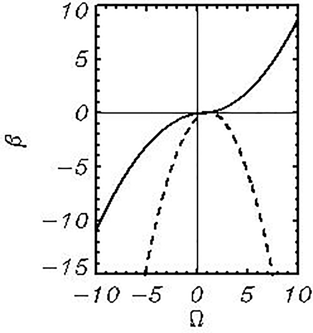
According to the linear theory (Miles, 1957), the Fourier components of surface pressure p are connected with those of the surface elevation through the following expression:

\begin{matrix} (14) & p_{k, l} + i p_{- k, - l} = \frac{ρ_{a}}{ρ_{w}} (β_{k, l} + i β_{- k, - l}) (h_{k, l} + i h_{- k, - l}), \end{matrix}

where $h_{k, l}, h_{- k, - l}, β_{k, l}, β_{- k, - l}$ are real and imaginary parts of elevation η and the so-called β function (i.e., Fourier coefficients at COS and SIN, respectively); ρ_a∕ρ_w is a ratio of the air and water densities. Equation (14) is a standard presentation of pressure above a multimode surface. It means that every wave mode with amplitude ${(h_{k, l}^{2} + h_{- k, - l}^{2})}^{1 / 2}$ initiates the pressure mode with amplitude ${(p_{k, l}^{2} + p_{- k, - l}^{2})}^{1 / 2}$ shifted off the phase of a wave mode by angle $α = atan \frac{β_{- k, - l}}{β_{k, l}}$ . Both coefficients in Eq. (14) are a function of the ratio of wind velocity at half the mode of the length height $λ_{k, l} / 2$ to the virtual phase velocity. Hence, for derivation of the shape of the β function it is necessary to simultaneously measure the wave surface elevation and the nonstatic pressure on the surface. Measurement of surface pressure is a very difficult problem since measurements should be carried out very close to a moving surface, preferably, with a surface-following sensor. Such measurements are performed quite seldom, especially, in the field. The measurements were carried out for the first time by a team of authors in both laboratory and field (Snyder et al., 1981; Hsiao and Shemdin, 1983; Hasselmann and Bösenberg, 1991; Donelan et al., 2005, 2006). The data obtained in this way allowed the construction of an imaginary part of the β function used in some versions of wave forecasting models (Rogers et al., 2012). Such measurements and their processing are quite complicated since the wave-produced pressure fluctuations are masked by the turbulent pressure fluctuations. The second method of the β function evaluation is based on the results of numerical investigations of the statistical structure of a boundary layer above waves with the use of Reynolds equations and an appropriate closure scheme. In general, this method works so well that many problems in the technical fluid mechanics are often solved using numerical models, not experimentally (Gent and Taylor, 1976; Riley et al., 1982; Al-Zanaidi and Hui, 1984). This method was being developed beginning from Chalikov (1978, 1986), followed by Chalikov and Makin (1991), Chalikov and Belevich (1992) and Chalikov (1995). The results were implemented in a WAVEWATCH model, i.e., a third-generation wave forecast model (Tolman and Chalikov, 1996), and thoroughly validated against the experimental data in the course of developing WAVEWATCH III (Tolman et al., 2014). This method was later improved on the basis of a more advanced coupled modeling of waves and boundary layer (Chalikov and Rainchik, 2010), while the β function used in WAVEWATCH III was corrected and extended up to the high frequencies. A direct calculation of the energy input to waves requires both the real and imaginary parts of the β function. The total energy input to waves depends on an imaginary part of the β function, while the moments of a higher order depend on both the imaginary and real parts of β. This is why a full approximation constructed in Chalikov and Rainchik (2010) was used in the current work. Note that in a range of relatively low frequencies the new method is very close to the scheme implemented in WAVEWATCH III.

It is a traditional suggestion that both coefficients are the functions of the virtual nondimensional frequency $Ω = ω_{k, l} U \cos ψ = U / c_{k, l} \cos ψ$ (where ω_k,l and U are the nondimensional radian frequency and wind speed, respectively; c_k,l is a phase speed of the kth mode; ψ is an angle between the wind and wave mode directions). Most of the schemes for calculations of the β function consider a relatively narrow interval of the nondimensional frequencies Ω. In the current work, the range of frequencies cover an interval $(0 < Ω < 10)$ , and occasionally the values of Ω>10 can appear. This is another reason why the function derived in Chalikov and Rainchik (2010) through the coupled simulations of waves and the boundary layer is used here. The wave model is based on the potential equations for a flow with a free surface, extended with an algorithm for the breaking dissipation (see below a description of the breaking dissipation parameterization). The wave boundary layer (WBL) model is based on Reynolds equations closed with a K−ε scheme; the solutions for air and water are matched through the interface. The β function was used for the evaluation of accuracy of the surface pressure p calculations. The shape of the β function connecting surface elevations and surface pressure is studied up to the high nondimensional wave frequencies in both positive and negative (i.e., for wind opposite to waves) domains. The data on the β function exhibit wide scatter, but since the volume of the data was quite large (47 long-term numerical runs allowed us to generate about 1 400 000 values of β), the shape of the β function was defined with satisfactory accuracy up to the very high nondimensional frequencies $(- 50 < Ω < 50)$ . As a result, the data on the β-function in such a broad range allow us to calculate the wave drag up to very high frequencies and to explicitly divide the fluxes of energy and momentum transferred by the pressure and molecular viscosity. This method is free of arbitrary assumptions on a drag coefficient C_d, and, conversely, such calculations allow the investigation of the nature of the wave drag (see Ting et al., 2012).

The most reliable data on β function are concentrated in the interval $- 10 < Ω < 10$ (negative values of Ω correspond to the wave modes running against wind). The real and imaginary parts of the β function are shown in Fig. 1. It is a corrected version of an approximation given in Chalikov and Rainchik (2010) in which the data at negative Ω were interpreted erroneously. In the current calculations the modes running against wind are absent. The function β can be approximated by the formulas

\begin{array}{l} (15) & β_{k, l} = \{\begin{array}{cc} β_{0} + a_{0} (Ω - Ω_{0}) + a_{1} {(Ω - Ω_{0})}^{2} & Ω_{0} < Ω \\ β_{0} + a_{0} (Ω - Ω_{0}) - a_{1} {(Ω - Ω_{0})}^{2} & Ω < Ω_{0} \end{array}, \\ (16) & β_{- k, - l} = \{\begin{array}{cc} β_{1} + a_{3} (Ω - Ω_{2}) & Ω < Ω_{2} \\ a_{2} {(Ω - Ω_{1})}^{2} & Ω_{2} < Ω < Ω_{3} \\ β_{1} - a_{3} (Ω - Ω_{3}) & Ω_{3} < Ω \end{array}, \end{array}

where the coefficients are $a_{1} = 0.09476, a_{2} = - 0.3718, a_{3} = 14.80, β_{0} = - 0.02, β = - 148 . a_{0} = 0.02277, Ω_{0} = 0.02277, Ω_{1} = 1.20, Ω_{2} = - 18.8, Ω_{3} = 21.2$ .

It was indicated above that an initial wave field is assigned as a superposition of linear modes whose amplitudes are calculated with a JONSWAP spectrum with an initial peak wave number $k_{p}^{0} = 100$ . An initial value $U / c_{p}^{0} = 6$ was chosen, i.e., a ratio of the nondimensional wind speed at the height of one-half the initial peak wave length $λ_{0} / 2 = 2 π / 100$ , and the phase speed $c_{p}^{0} = {(k_{p}^{0})}^{- 1 / 2}$ is equal to 6. Such a high ratio corresponds to the initial stages of wave development. The wind velocity $6 c_{p}^{0}$ remains constant throughout the integration. The values of Ω for other wave numbers are calculated by assuming that the wind profile is logarithmic:

\begin{matrix} (17) & Ω_{k, l} = \frac{U}{c_{k, l}} \ln \frac{λ_{k, l}}{2 z_{0}} {(\ln \frac{λ_{0}}{2 z_{00}})}^{- 1} \cos ψ_{k, l}, \end{matrix}

where z₀₀ is an effective nondimensional roughness for the initial wind profile, while z₀ is an actual roughness parameter that depends on the energy in a high-frequency part of the spectrum and on the wind profile. We call it “effective” since very close to the surface the wind profile is not logarithmic (Chalikov, 1995; Tolman and Chalikov, 1996; Chalikov and Rainchik, 2010). The value of this parameter depends on the wind velocity and energy in a high-wave-number interval of the wave spectrum, as well as on the length scale of the problem. All these effects are possible to include by matching the wave model with a one-dimensional WBL model (Ting et al., 2012). Here, a simplified scheme for the roughness parameter is chosen. It is well known that the roughness parameter (as well as a drag coefficient) increases with a decrease in the inverse wave age. In our case the wind speed is fixed, and dependence for a nondimensional roughness parameter is constructed on the basis of the results obtained in Chalikov and Rainchik (2010):

\begin{matrix} (18) & z_{0} = 15 z_{00} Ω, \end{matrix}

where $z_{00} = 10^{- 3}$ is an initial value of the roughness parameter. Equation (18) approximates the dependence of the effective roughness at the stage of wave development. Note that the results are not sensitive to the variation of the roughness parameter within reasonable limits.

https://www.ocean-sci.net/14/453/2018/os-14-453-2018-f01

Figure 1Real (dashed curve) and imaginary (solid curve) parts of the β function.

Download

3.2 High-wave-number energy dissipation

A nonlinear flux of energy directed to the small wave numbers produces the downshifting of the spectrum, while an opposite flux forms the shape of the spectral tail. The second process can produce the accumulation of energy near a “cut” wave number. Both processes become more intensive with an increase in the energy input. The growth of amplitudes at high wave numbers is followed by that of the local steepness and numerical instability. This well-known phenomenon in the numerical fluid mechanics is eliminated by use of a highly selective filter simulating the nonlinear viscosity. To support stability, additional terms are included in the right-hand sides of Eqs. (4) and (5):

\begin{array}{l} (19) & \frac{\partial η_{k, l}}{\partial τ} = E_{k, l} - μ_{k, l} η_{k, l}, \\ (20) & \frac{\partial φ_{k, l}}{\partial τ} = F_{k, l} - μ_{k, l} φ_{k, l} . \end{array}

E_k,l and F_k,l are the Fourier amplitudes of the right-hand sides of Eqs. (4) and (5) while a factor μ_k,l is calculated using the formula

\begin{matrix} (21) & µ_{k, l} = \{\begin{array}{cc} 0 & |k| < k_{d} \\ c_{m} k_{0} {(\frac{|k| - k_{d}}{(k_{0} - k_{d})})}^{2} & k_{d} \leq |k| \leq k_{0} \\ c_{m} k_{0} & |k| > k_{0} \end{array}, \end{matrix}

where k and l are components of wave number |k|, while the coefficients k_d and k₀ are defined by the expression:

\begin{matrix} (22) & k_{d} = d_{m}^{2} M_{x} M_{y} {({(l {|k|}^{- 1} d_{m} M_{x})}^{2} + {(k {|k|}^{- 1} d_{m} M_{y})}^{2})}^{- 1 / 2}, \end{matrix}

\begin{matrix} (23) & k_{0} = M_{x} M_{y} {({(l {|k|}^{- 1} M_{x})}^{2} + {(k {|k|}^{- 1} M_{y})}^{2})}^{- 1 / 2}, \end{matrix}

where c_m=0.1 and d_m=0.75. The expressions (19)–(21) can be interpreted in a straightforward way: the value of µ_k,l is equal to zero inside the ellipse with semiaxes d_mM_x and d_mM_y; then it grows linearly with |k| up to the value c_m and is equal to c_m outside the outer ellipse. This method of filtration that we call “tail dissipation” was developed and validated with a conformal model by Chalikov and Sheinin (1998). The sensitivity of the results to the parameters in Eqs. (21)–(23) is not high. The aim of the algorithm is to support smoothness and monotonicity of the wave spectrum within a high wave number range. Since the algorithm affects the amplitudes of small modes, it actually does not reduce the total energy, though it efficiently prevents development of the numerical instability. Note that no long-term calculations can be performed without tail dissipation eliminating the development of numerical instability at high wave numbers.

3.3 Dissipation due to wave breaking

The main process of wave dissipation is wave breaking. This process is taken into account in all the spectral wave forecasting models similar to WAVEWATCH (see Tolman and Chalikov, 1996). Since there are no waves in the spectral models, no local criteria of wave breaking can be formulated. This is why the breaking dissipation is represented in spectral models in a distorted form. A real breaking occurs in relatively narrow areas of the physical space; however, a spectral image of such breaking is stretched over the entire wave spectrum, while in reality the breaking decreases height and energy of dominant waves. This contradiction occurs because the waves in spectral models are assumed to be the linear ones, while in fact the breaking occurs in the physical space with a nonlinear sharp wave, usually composed of several modes. However, progress has been gradually made in spectral wave modeling over the past decade. It became clear that state-of-the-art wave models should account for the threshold behavior of the dominant wave breaking, i.e., waves will not break unless their steepness exceeds the threshold (Alves and Banner, 2003; Babanin et al., 2010).

The mechanics of wave breaking at a developed wave spectrum differs from that in a wave field represented by the few modes normally considered in many theoretical and laboratory investigations (e.g., Alberello et al., 2018). Since the breaking in laboratory conditions is initiated by special assignment of amplitudes and phases, it cannot be similar to the breaking in natural conditions. To some degree the wave breaking is similar to the development of an extreme wave that appears suddenly with no pronounced prehistory (Chalikov and Babanin, 2016a, b). There are no signs of modulational instability in both phenomena, which suggests a process of energy consumption from other modes. The evolution leading to the breaking or “freaking” seems just opposite: the full energy of a main wave remains nearly constant while the columnar energy is focused around the crest of this wave, which becomes sharper and unstable. Probably even more frequent cases of wave breaking and extreme wave appearance can be explained by a local superposition of several modes.

The instability of interface leading to the breaking is an important and poorly developed problem of fluid mechanics. In general, this essentially nonlinear process should be investigated for a two-phase flow. Such an approach was demonstrated, for example, by Iafrati (2009). However, progress in solving this highly complicated problem is slow.

A problem of the breaking parameterization includes two points: (1) establishing of a criterion of the breaking onset and (2) development of an algorithm of the breaking parameterization. The problem of breaking is discussed in detail in Babanin (2011). Chalikov and Babanin (2012) performed a numerical investigation of the processes leading to the breaking. It was found that a clear predictor of the breaking formulated in dynamical and geometrical terms probably does not exist. The most evident criterion of the breaking is the breaking itself, i.e., the process when some part of the upper portion of a sharp wave crest is falling down. This process is usually followed by separation of the detached volume of liquid into the water and air phases. Unfortunately, there is no possibility of describing this process within the scope of the potential theory.

Some investigators suggest using a physical velocity approaching the rate of surface movement in the same direction as a criterion of the breaking onset. This is incorrect since a kinematic boundary condition suggests that these quantities are exactly equal to each other. It is quite clear that the onset of breaking can be characterized by the appearance of a non-single-value piece of surface. This stage can be investigated with a two-dimensional model, which due to a high flexibility of the conformal coordinates allows us to reproduce a surface with an inclination in the Cartesian coordinates exceeding 90 degrees. (In the conformal coordinates the dependence of elevation on a curvilinear coordinate is always a single value). The duration of this stage is extremely short, the calculations being always interrupted by the numerical instability with sharp violation of the conservation laws (constant integral invariants, i.e., full energy and volume) and strong distortion of the local structure of flow. The numerous numerical experiments with a conformal model showed that after the appearance of a non-single value the model never returns to stability. However, the introduction of a non-single surface as a criterion of the breaking instability even in a conformal model is impossible since a behavior of the model at a critical point is unpredictable, and the run is most likely to be terminated, no matter what kind of parameterization of breaking is introduced. It means that even in a precise conformal model the stabilization of the solution should be initiated prior to the breaking.

A consideration of an exact criterion for the breaking onset for the models using transformation of the coordinate type of point (1) is useless since the numerical instability in such models arises not because of the approach of breaking but because of the appearance of large local steepness. The multiple experiments with a direct 3-D wave model show that the appearance of the local steepness $max (\partial η / \partial x, \partial η / \partial y)$ exceeding ≈2 (that corresponds to a slope of about 60 degrees) is always followed by the numerical instability but the instability can happen well before reaching this value. The decrease in a time step does not make any effect. As seen, a surface with such a slope is very far from being a vertical wall, when the real breaking starts. However, an algorithm for the breaking parameterization must prevent numerical instability. The situation is similar to the numerical modeling of turbulence (LES technique) in which a local highly selective viscosity is used to prevent the appearance of too large local gradients of the velocity. A description of the breaking in the direct wave modeling should satisfy the following conditions. (1) It should prevent the onset of instability at each point of half a million grid points over more than 100 thousand time steps. (2) It should describe in a more or less realistic way the loss of kinetic and potential energies with preservation of balance between them. (3) It should preserve the volume. It was suggested in Chalikov (2005) that an acceptable scheme can be based on a local highly selective diffusion operator with a special diffusion coefficient. Several schemes of such type were validated, and finally the following scheme was chosen:

\begin{array}{l} (24) & η_{τ} = E_{η} + J^{- 1} (\frac{\partial}{\partial ξ} B_{ξ} \frac{\partial η}{\partial ξ} + \frac{\partial}{\partial ϑ} B_{ϑ} \frac{\partial η}{\partial ϑ}), \\ (25) & φ_{τ} = F_{φ} + J^{- 1} (\frac{\partial}{\partial ξ} B_{ξ} \frac{\partial φ}{\partial ξ} + \frac{\partial}{\partial ϑ} B_{ϑ} \frac{\partial φ}{\partial ϑ}), \end{array}

where F_η and F_φ are the right-hand sides of Eqs. (4) and (5) including the terms introduced in terms of Fourier coefficients by Eqs. (19)–(23); B_ξ and B_ϑ are diffusion coefficients. It was suggested in the first versions of the scheme that a diffusion coefficient depends on a local slope; however, such a scheme did not prove to be very reliable since it did not prevent all of the events of the numerical instability. A scheme based on the calculation of the local curvilinearity η_ξξ and η_ϑϑ turned out to be a lot more robust. The calculations of 75 different runs were performed with a full 3-D model in Chalikov et al. (2014) over the period of t=350 (70 000 time steps). The total number of values used for the calculations of dependence in Fig. 2 (thick curve) is about 6 billion. The normal probability calculated with the same dispersion is shown by a thin curve.

It is seen that the probability of large negative values of the curvilinearity is calculated over an ensemble of linear modes by orders larger than the probability with the spectra generated by a nonlinear model.

The curvilinearity turned out to be very sensitive to the shape of surface. This is why it was chosen as a criterion of the breaking approach. Coefficients B_ξ and B_ϑ depend nonlinearly on the curvilinearity:

\begin{array}{l} (26) & B_{ξ} = \{\begin{array}{cc} Δ ξ C_{B} η_{ξ ξ}^{2} & η_{ξ ξ} < η_{ξ ξ}^{c r} \\ 0 & η_{ξ ξ} \geq η_{ξ ξ}^{c r} \end{array}, \\ (27) & B_{ϑ} = \{\begin{array}{cc} Δ ϑ C_{B} η_{ϑ ϑ}^{2} & η_{ϑ ϑ} < η_{ξ ξ}^{c r} \\ 0 & η_{ϑ ϑ} \geq η_{ξ ξ}^{c r} \end{array}, \end{array}

where Δξ and Δζ are the horizontal steps in the x and y directions in a grid space, and the coefficients are C_B=2.0 and $η_{ξ ξ}^{c r} = η_{ϑ ϑ}^{c r} = - 50$ . Equations (24)–(27) do not change the volume and decrease the local potential and kinetic energy. It is assumed that the lost momentum and energy are transferred to the current and turbulence (see Chalikov and Belevich, 1992). In addition, the energy also goes to other wave modes. The choice of parameters in Eqs. (24)–(27) is based on simple considerations: a local piece of surface can closely approach the critical curvilinearity but not exceed it. The values of the coefficients are picked with reserve to provide stability for long runs.

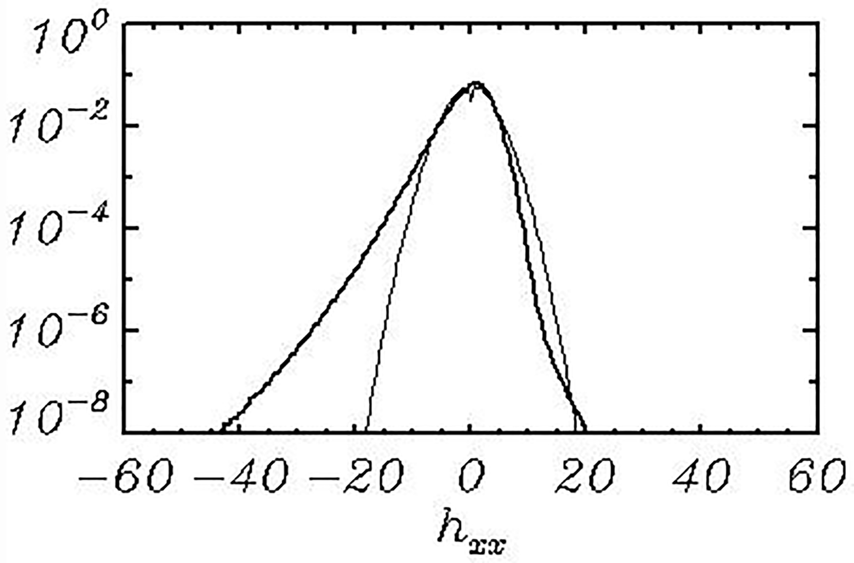
https://www.ocean-sci.net/14/453/2018/os-14-453-2018-f02

Figure 2Probability of the curvilinearity η_ξξ. The thick curve is calculated with a full 3-D model; the thin curve is the probability calculated over an ensemble of linear modes with the same spectrum.

Download

We do not think that the suggested breaking parameterization is a final solution to the problem. Other schemes will be tested in the next version of the model. However, the results presented below show that the scheme is reliable and provides a realistic energy dissipation rate.

4 Calculations and results

The elevation and surface velocity potential fields are approximated in the current calculations by M_x=256 and M_y=128 modes in directions x and y. The corresponding grid includes $N_{x} \times N_{y} = (1024 \times 512)$ knots. The vertical derivatives are approximated at a vertical stretched grid $d ζ_{j + 1} = χ d ζ_{j}, (j = 1, 2, 3 \dots, L_{w})$ , where ν=1.2 and L_w=10. A small number of levels used for the solution of the equation for a nonlinear component of the velocity potential are possible because just a surface vertical derivative for the velocity potential $\partial Φ / \partial ζ (ζ = 0)$ is required. The velocity potential mainly consists of an analytical component $\bar{φ}$ , while a nonlinear component provides only a small correction. To reach the accuracy of the solution $ε = 10^{- 6}$ for Eq. (11), no more than two iterations were usually sufficient.

The parameters chosen were used for solution of a problem of a wave field evolution over the acceptable time (of the order of 10 days). The initial conditions were assigned on the basis of the empirical spectrum JONSWAP (Hasselmann et al., 1973) with a maximum placed at the wave number k_p=100 with the angle spreading (coshψ)²⁵⁶. The details of the initial conditions are of no importance because an initial energy level is quite low.

The total energy of a wave motion $E = E_{p} + E_{k}$ (E_p is a potential energy, while E_k is a kinetic energy) is calculated with the following formulas:

\begin{matrix} (28) & E_{p} = 0.25 \overline{η^{2}}, E_{k} = 0.5 \overline{\overline{(φ_{x}^{2} + φ_{y}^{2} + φ_{z}^{2})}}, \end{matrix}

where a single bar denotes averaging over the ξ and ϑ coordinates, and a double bar denotes averaging over the entire volume. The derivatives in Eq. (25) are calculated according to the transformation (1). An equation of the integral energy $E = E_{p} + E_{k}$ evolution can be represented in the following form:

\begin{matrix} (29) & \frac{d E}{d t} = \overline{\overline{I}} + \overline{\overline{D_{b}}} + \overline{\overline{D_{t}}} + \overline{\overline{N}}, \end{matrix}

where $\overline{\overline{I}}$ is the integral input of energy from wind (Eqs. 14–18); $\overline{\overline{D_{b}}}$ is the rate of the energy dissipation due to the wave breaking (Eqs. 24–27); $\overline{\overline{D_{t}}}$ is the rate of the energy dissipation due to filtration of high-wave-number modes (tail dissipation, Eqs. 19–23); $\overline{\overline{N}}$ is an integral effect of the nonlinear interactions described by the right-hand side of the equations when the surface pressure p is equal to zero. The differential form for calculation of the energy transformation can be, in principle, derived from Eqs. (4)–(6), but here a more convenient and simple method was applied. Different rates of the integral energy transformations can be calculated with the help of fictitious time steps (i.e., apart from the basic calculations). For example, the value of $\overline{\overline{I}}$ is calculated by the following relation:

\begin{matrix} (30) & \overline{\overline{I}} = \frac{1}{Δ t} (\overline{\overline{E^{t + Δ t}}} - \overline{\overline{E^{t}}}), \end{matrix}

where $\overline{\overline{E^{t + Δ t}}}$ is the integral energy of a wave field obtained after one time step with the right side of Eq. (6) containing only the surface pressure calculated with Eqs. (14)–(18). For calculation of the dissipation rate due to filtration, the right-hand side of the equations contains just the terms introduced in Eqs. (19)–(23), while for calculation of the effects of breaking, only the terms introduced in Eqs. (24)–(27) are in use.

An evolution of the characteristics calculated by Eq. (30) is shown in Fig. 3. The sharp variations in all the characteristics at t<50 can probably be explained by adjustment of the initial linear fields to the nonlinearity. Up to the end of integration, the sum of all energy transition terms (tail dissipation $\overline{\overline{D_{t}}}$ , breaking dissipation $\overline{\overline{D_{b}}}$ and energy input $\overline{\overline{I}})$ approaches zero (curve 4), and the energy growth E (curve 5) stops. Then the energy tends to decrease, but we are not sure about the nature of this effect. Such behavior can be explained by a fluctuating character of mutual adjustment of input and dissipation or simply by deterioration of the approximation because of the downshifting process. Note that opposite to a more or less monotonic behavior of the tail dissipation (curve 1), the breaking dissipation is highly intermittent, which is consistent with the common views on the wave breaking nature.

The data on the evolution of the wave spectrum are shown in Fig. 4. A 2-D wave spectrum S(k,l) $(0 \leq k \leq M_{x}, - M_{y} \leq l \leq M_{y})$ averaged over 13 time intervals of length equal to Δt≈100 was transferred to the polar coordinates $S_{p} (ψ, r) (- π / 2 \leq ψ \leq π / 2, 0 \leq r \leq M_{x})$ and then averaged over the angle ψ to obtain a 1-D spectrum S_h(r):

\begin{matrix} (31) & S_{h} (r) = \sum S_{p} (ψ, r) r Δ ψ . \end{matrix}

An angle ψ=0 coincides with the direction of wind U, $Δ ψ = π / 180 .$

https://www.ocean-sci.net/14/453/2018/os-14-453-2018-f03

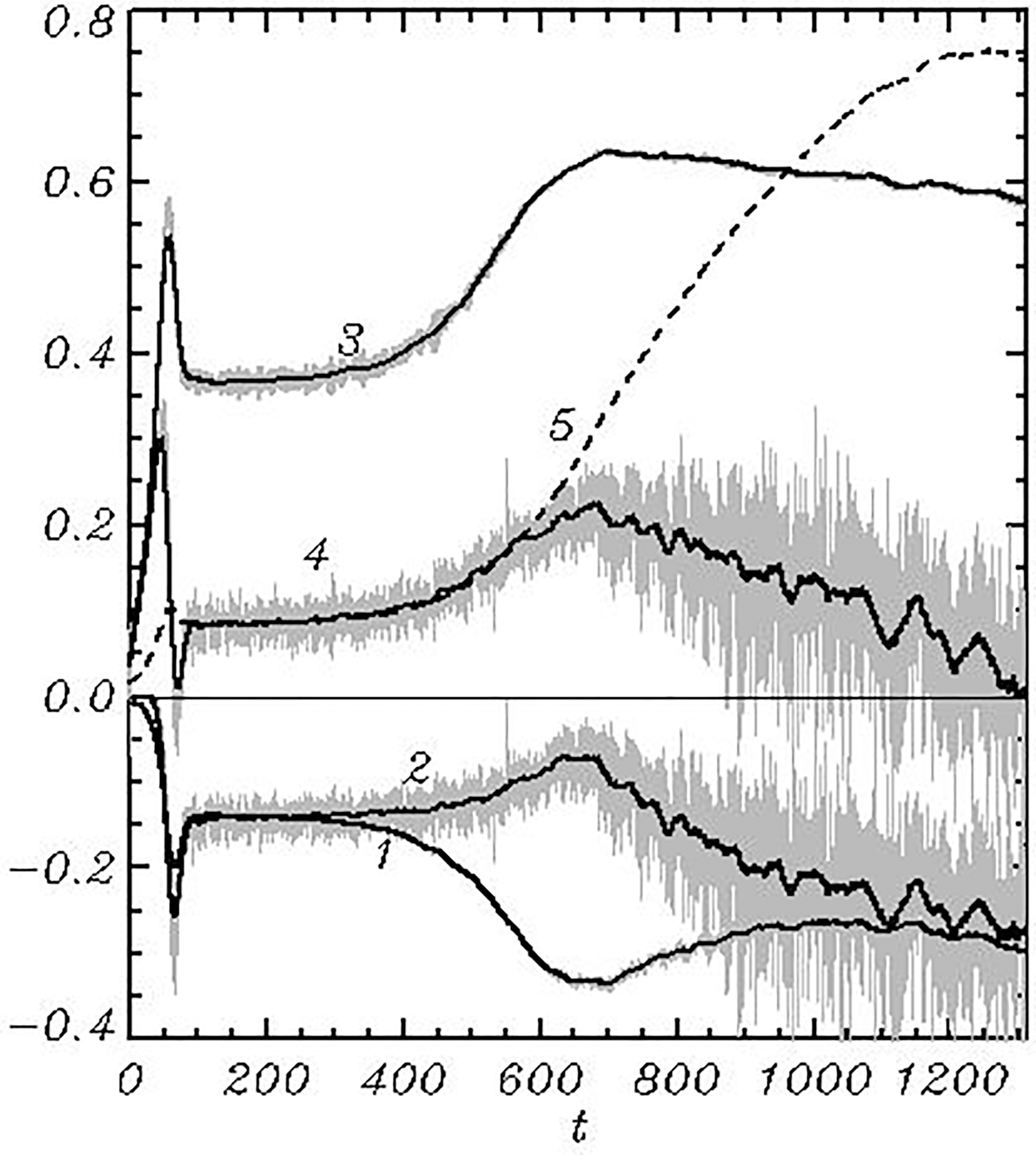
Figure 3Evolution of integral characteristics of the solution, a rate of evolution of the integral energy multiplied by 10⁷ due to 1 – tail dissipation D_t (Eqs. 19–23), 2 – breaking dissipation D_b (Eqs. 24–27), 3 – input of energy from wind I (Eqs. 14–18) and 4 – balance of energy $I + D_{t} + D_{b}$ . Curve 5 shows the evolution of wave energy 10⁵E. Grey vertical bars show the instantaneous values; the thick curve shows the smoothed behavior.

Download

https://www.ocean-sci.net/14/453/2018/os-14-453-2018-f04

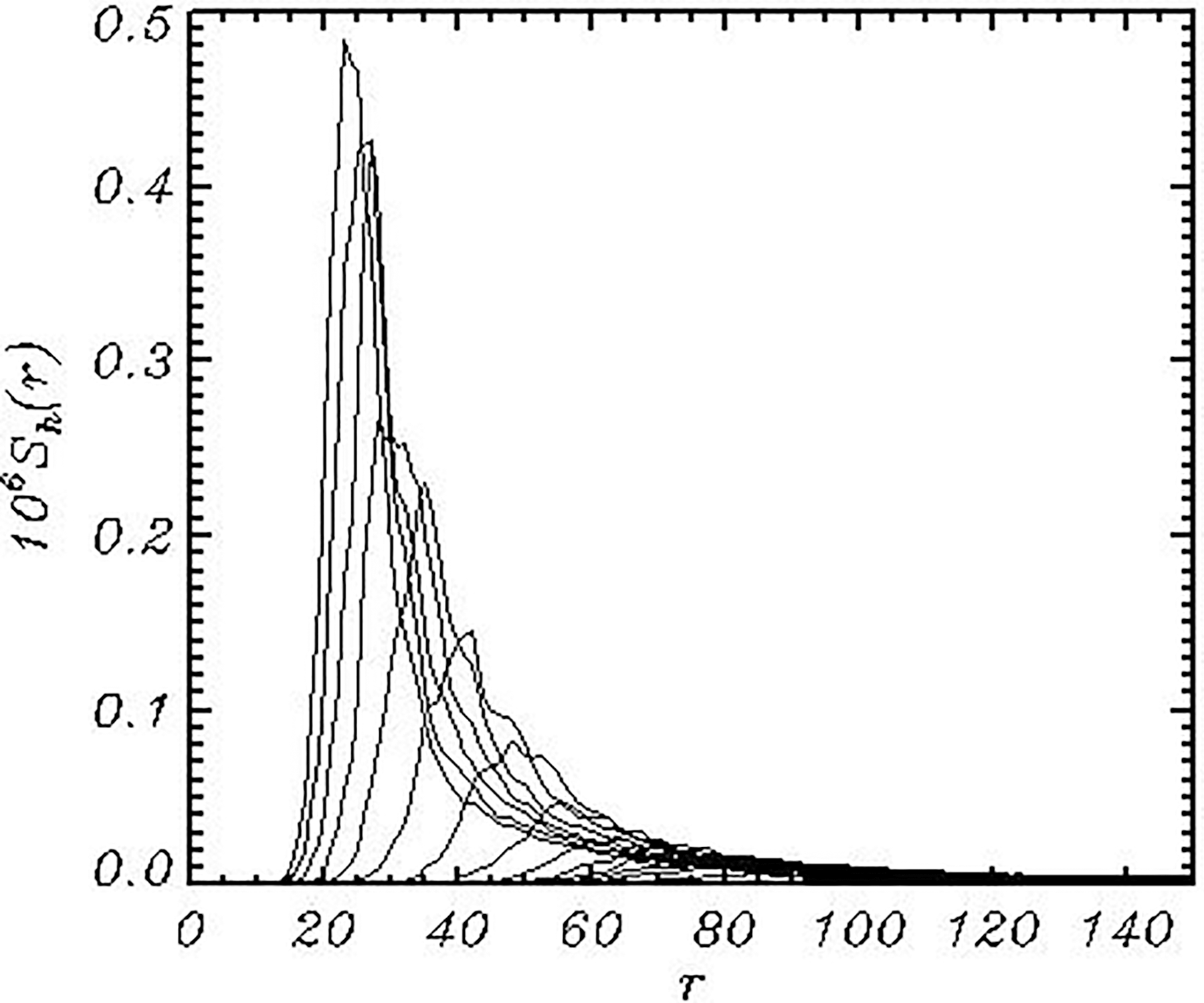
Figure 4The wave spectra S_h(r) integrated over angle ψ in the polar coordinates and averaged over the consequent intervals of length for about 100 units of the nondimensional time t. The spectra grow and shift from right to left.

Download

As seen, each spectrum consists of separated peaks and holes¹. This phenomenon was first observed and discussed by Chalikov et al. (2014). The repeated calculations with different resolution showed that such a structure of the 2-D spectrum is typical. It cannot be explained by a fixed combination of interacting modes since in different runs (with the same initial conditions but a different set of phases for the modes) the peaks are located at different locations in a Fourier space.

Another presentation is given in Fig. 6 in which the log₁₀(S(ψ,r)), averaged over the successive seven-period length Δt=200, is given. The first panel with a mark of 0 refers to the initial conditions. The disturbances within the range ( $125 < k < 150$ ) reflect the initial adjustment of input and dissipation at a high-wave-number slope of spectrum. The pictures characterize the downshifting and angle spreading of the spectrum well due to the nonlinear interactions.

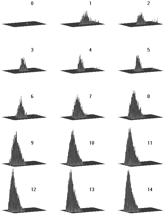
https://www.ocean-sci.net/14/453/2018/os-14-453-2018-f05

Figure 5Sequence of 3-D images of lg₁₀(S(k,l)), in which each panel corresponds to a single curve in Fig. 3. The left side refers to the wave number $l (- M_{y} \leq l \leq M_{y})$ and the front side refers to $k (0 \leq k \leq M)$ . The numbers indicate the end of the time interval expressed in hundreds of nondimensional time units.

Download

https://www.ocean-sci.net/14/453/2018/os-14-453-2018-f06

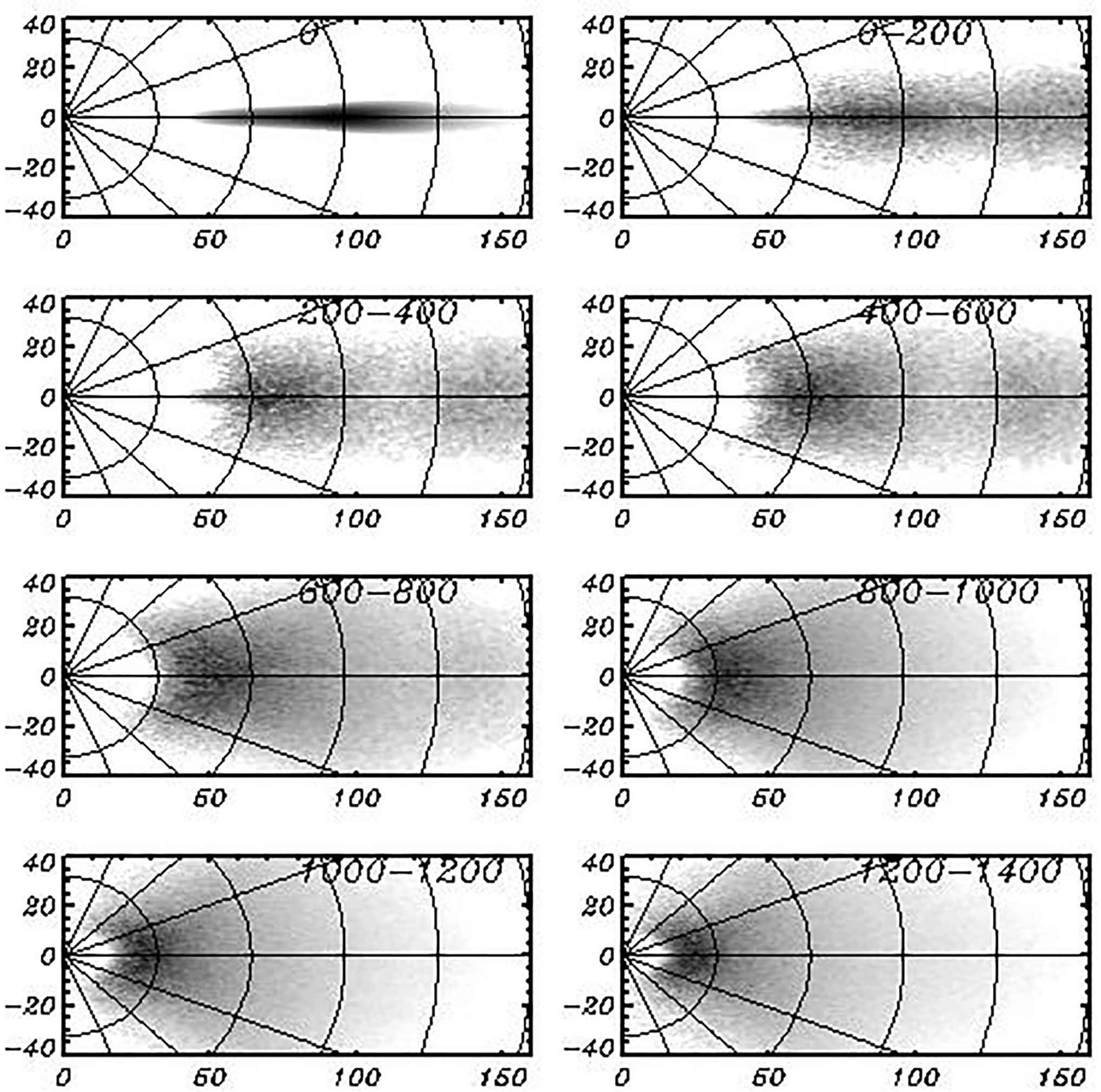
Figure 6Sequence of 2-D images of lg₁₀(S(k,l)) averaged over the consequent seven periods of length Δt=200. The numbers indicate the period of averaging (first panel marked 0, refers to the initial conditions). The horizontal and vertical axes correspond to the wave numbers k and l, respectively.

Download

Evolution of the integrated-over-angles ψ wave spectrum S_h(r) can be described with the equation

\begin{matrix} (32) & \frac{d S_{h} (r)}{d t} = I (r) + D_{t} (r) + D_{b} (r) + N (r), \end{matrix}

where $I (r), D_{t} (r), D_{b} (r) and N (r)$ are the spectra of the input energy, tail dissipation, breaking dissipation and the rate of the nonlinear interactions, all obtained by integration over angles ψ. All of the spectra shown below were obtained by transformation of the 2-D spectra into a polar coordinate (ψ,r) and then integrated over angles ψ within the interval $(- π / 2, π / 2)$ . The spectra can be calculated using an algorithm similar to that (Eq. 30) for integral characteristics. For example, a spectrum of the energy input I(k,l) is calculated as follows:

\begin{matrix} (33) & I (k, l) = (S_{c}^{t + Δ t} (k, l) - S_{c}^{t} (k, l)) / Δ t, \end{matrix}

where S_c(k_x,k_y) is the spectrum of the columnar energy calculated by the relation

\begin{array}{l} S_{c} (k, l) = \frac{1}{2} (h_{k, l}^{2} + h_{- k, - l}^{2} + \int_{- H}^{0} . \\ (34) & (u_{k, l}^{2} + u_{- k, - l}^{2} + v_{k, l}^{2} + v_{- k, - l}^{2} + w_{k, l}^{2} + w_{- k, - l}^{2}) d ζ), \end{array}

where the grid values of velocity components u,v and w are calculated by the relations

\begin{matrix} (35) & u = φ_{ξ} + φ_{ζ} η_{ξ}, v = φ_{ϑ} + φ_{ζ} η_{ϑ}, w = φ_{ζ}, \end{matrix}

and $u_{k, l}, v_{k, l} and w_{k, l}$ are their Fourier coefficients.

For calculation of I(k,l) the fictitious time steps Δt are made only with a term responsible for the energy input, i.e., surface pressure p. A spectrum I(k,l) was averaged over the periods Δt≈100, then transformed into a polar coordinate system and integrated in a Fourier space over angles ψ within the interval $(- π / 2, π / 2) .$

Evolution of the input spectra (Fig. 7) is in general similar to that of the wave spectra shown in Fig. 4. Note that the maximum of the spectra is located at the maximum of the wave spectra since the input depends mainly on the spectral density, while the dependence on frequency is less important.

An algorithm (Eq. 30) was applied for calculation of the dissipation spectra due to dumping of a high-wave-number part of spectrum (tail dissipation) and for calculation of the spectrum of the breaking dissipation. In the first case, the fictitious time step was made taking into account the terms described by Eqs. (19)–(23), while in the second case the time step was made using the terms described by Eqs. (24)–(27).

The spectra of the tail dissipation calculated similarly to the spectra I(r) are shown in Fig. 8. The dissipation occurs at the periphery of the spectrum, outside an ellipse with semiaxes d_mM_x and d_mM_y². This is why such dissipation, averaged over angles, seems to affect the middle part of a 1-D spectrum. The tail dissipation effectively stabilizes the solution.

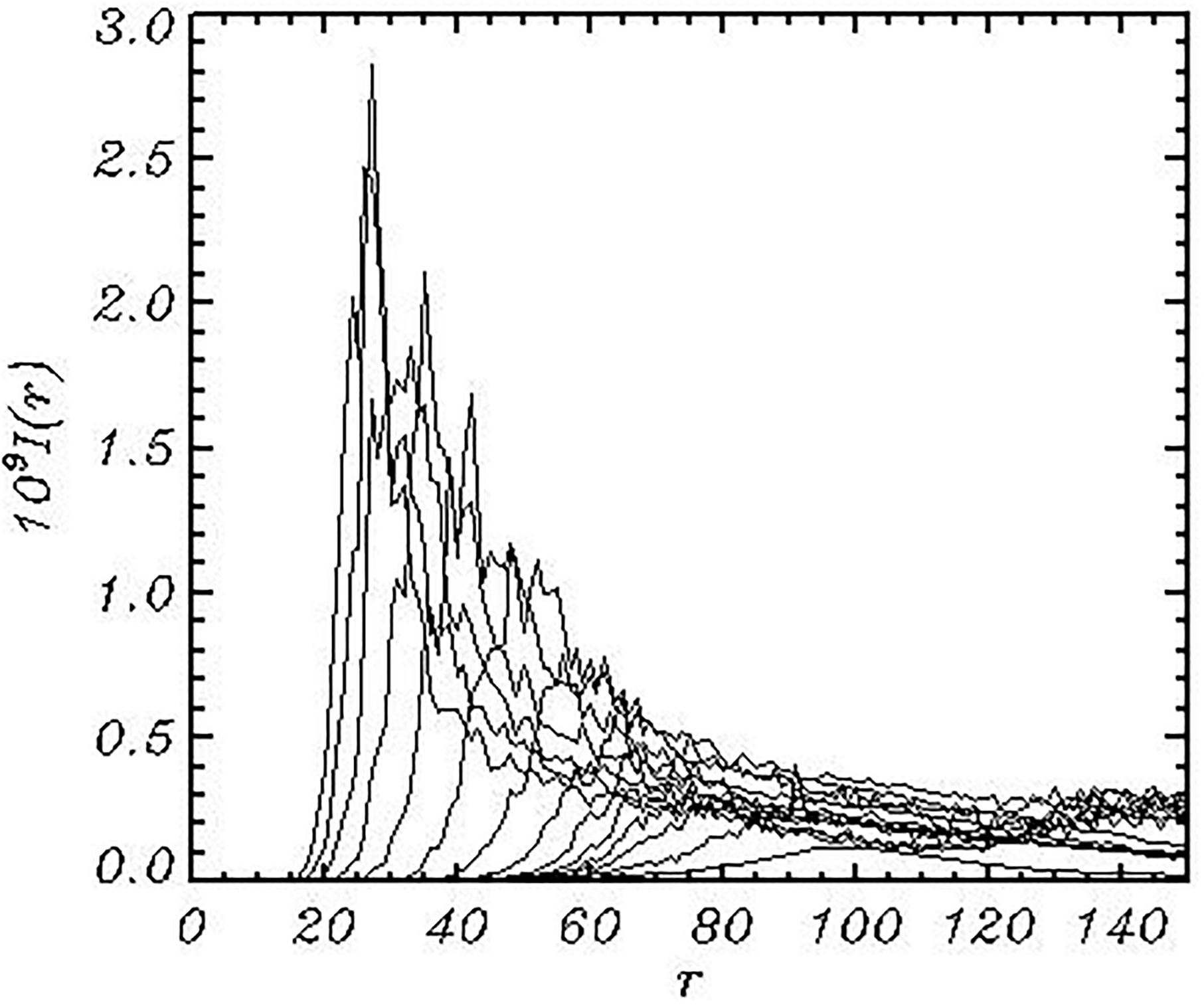
https://www.ocean-sci.net/14/453/2018/os-14-453-2018-f07

Figure 7The spectrum of energy input I(r) integrated over angle ψ in the polar coordinates and averaged over the consequent intervals of length for about 100 units of the nondimensional time t.

Download

https://www.ocean-sci.net/14/453/2018/os-14-453-2018-f08

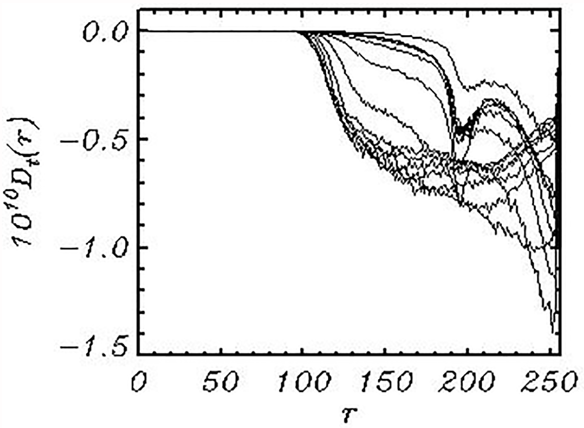
Figure 8The tail dissipation spectra D_t(r) integrated over angle ψ in the polar coordinates and averaged over the consequent intervals of length for about 100 units of the nondimensional time t.

Download

The breaking dissipation averaged over angles is presented in Fig. 8. As seen, the breaking dissipation has a maximum at the spectral peak. This does not mean that in the vicinity of the wave peak the probability of large curvilinearity is quite high. A high rate of the breaking dissipation can be explained by high wave energy in the vicinity of the wave peak. The energy lost through the breaking, described by the diffusion mechanism, correlates with the energy of breaking waves. Opposite to the high-wave-number dissipation which regulates the shape of the spectral tail, the breaking dissipation forms the main energy-containing part of the spectrum.

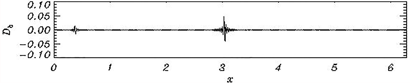
The diffusion mechanism suggested in Eqs. (24)–(27) modifies an elevation and surface stream function in close vicinity of the breaking point. The amplitudes of side perturbation are small and decrease very quickly throughout the distance from the breaking point.

An example of the profile of the energy input due to the breaking D_b(x) is given in Fig. 10. As seen, the energy input fluctuates around the breaking point. A diffusion operator chosen for the breaking parameterization not only decreases total energy but also redistributes the energy between Fourier modes in a Fourier space.

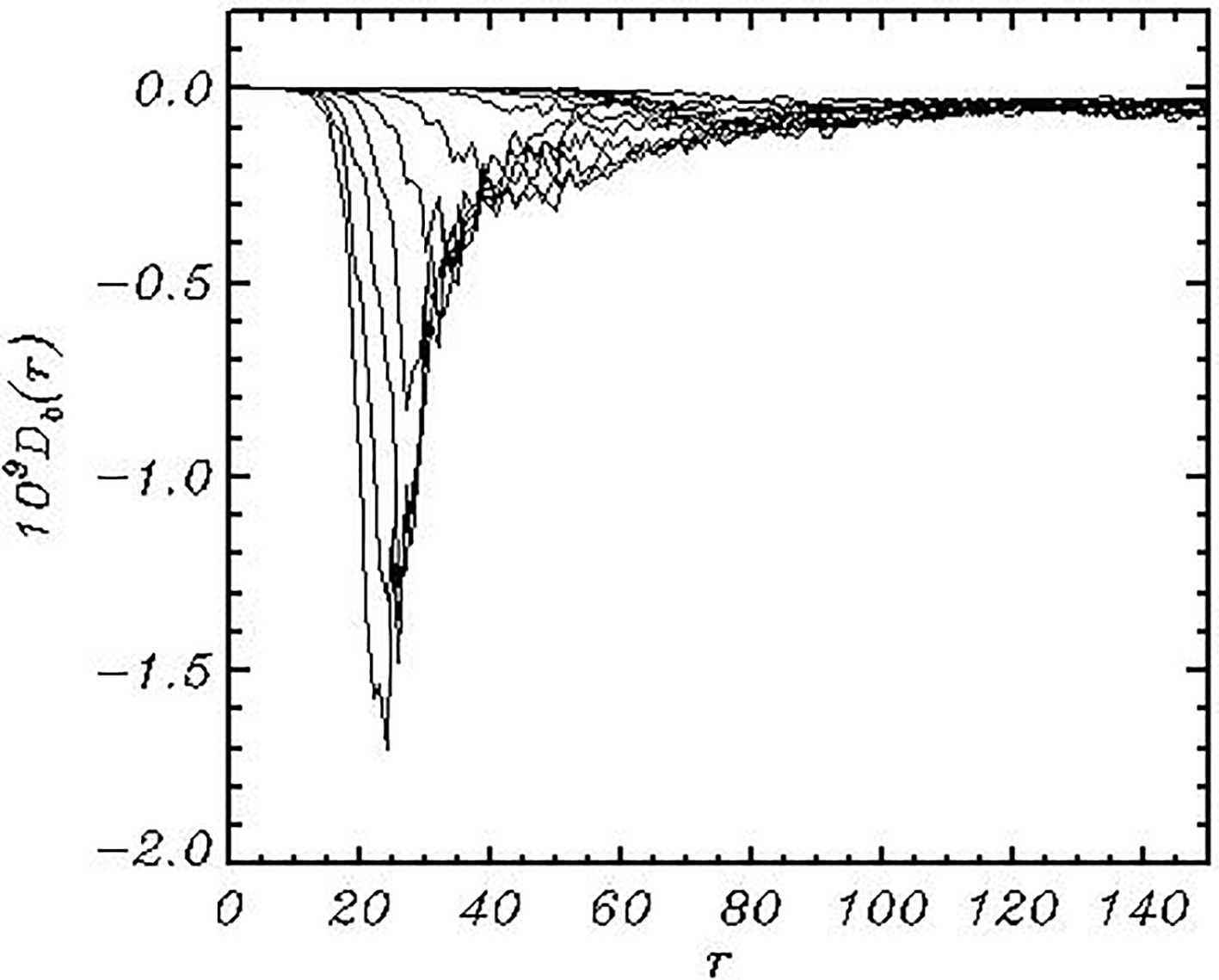
https://www.ocean-sci.net/14/453/2018/os-14-453-2018-f09

Figure 9The breaking dissipation spectra D_b(r) integrated over angle ψ in the polar coordinates and averaged over the consequent intervals of length for about 100 units of the nondimensional time t.

Download

In general, for the specific conditions considered in this paper, the breaking is an occasional process taking place in a small part of the domain. The kurtosis of the input energy due to the breaking D_b(ξ,ϑ), i.e., the value

\begin{matrix} (36) & Ku = \overline{\overline{D_{b}^{4}}} {(\overline{\overline{D_{b}^{2}}})}^{- 2} - 3, \end{matrix}

is of the order of 10³, which corresponds to a plain function with occasional separated peaks.

The number of breaking points in terms of percentage of the total number of points is given in Fig. 11. As seen, the number of breaking events decreases to t=600 and then increases till the end of the calculations. The number of breaking events is not directly connected with the intensity of breaking, which is seen when comparing Fig. 11 and curve 2 in Fig. 3.

An integral term describing a nonlinear interaction $\overline{\overline{N}}$ in Eq. (29) is small (compared with the local values of N_k,l), but the magnitude of spectrum N(r) is comparable with input I(r) and dissipation terms D_t(r) and D_b(r). The presentation of term N(r) in the form shown in Figs. 6–8 is not clear. This is why the spectra 10⁸N(r) averaged over interval Δt=100 are plotted separately in Fig. 11 for the last eight intervals (thick curves) together with a wave spectrum 10⁶S_h(r). In general, the shapes of spectrum N(r) agree with the conclusions of the quasi-linear Hasselmann (1962) theory (Hasselmann et al., 1985). At a low-wave-number slope of spectrum the nonlinear influx of energy is positive, while at the opposite slope it is negative. This process produces the shifting of the spectrum to a lower wave number (downshifting). Opposite to the Hasselmann's theory, these results are obtained by solution of the full three-dimensional equations. It would be interesting to compare our results with the calculations of Hasselmann's integral. Unfortunately, neither of the existing programs of such a type permits calculations with the high resolution that was used in the current model. Note that the nonlinear interactions also produce widening of the spectrum.

https://www.ocean-sci.net/14/453/2018/os-14-453-2018-f10

Figure 10Example of the energy input due to the breaking D_b(x).

Download

As can be seen, the nonlinearity is quite an important property of surface waves. The contribution of nonlinearity can be estimated, for example, by comparison of the kinetic energy of a linear component $E_{l} = 0.5 \overline{\overline{({\bar{φ}}_{x}^{2} + {\bar{φ}}_{y}^{2} + {\bar{φ}}_{z}^{2})}}$ and the total kinetic energy E_k (Fig. 13). A ratio E_l∕E_k as a function of time remains very close to 1, which proves that the nonlinear part of energy makes up just a small percentage of the total energy. It does not mean that the role of the nonlinearity is small; its influence can manifest itself over large timescales.

The time evolution of the integral spectral characteristics is presented in Fig. 14. Curve 1 corresponds to the weighted frequency ω_w

\begin{matrix} (37) & ω_{w} = {(\frac{\int k S d k d l}{\int S d k d l})}^{1 / 2}, \end{matrix}

where integrals are taken over the entire Fourier domain. The value ω_w is not sensitive to the details of the spectrum; hence, it characterizes the position of spectrum and its shifting well. Curve 2 describes an evolution of the spectral maximum. The step shape of the curve corresponds to the fundamental property of downshifting. Opposite to the common views, the development of spectrum occurs not monotonically but by the appearance of a new maximum at a lower wave number as well as by attenuation of the previous maximum. It is interesting to note that the same phenomenon is also observed in a spectral model (Rogers et al., 2012). Curve 3 describes the change of total energy $E = E_{p} + E_{k}$ . As seen, all three curves have a tendency to slow down the evolution rate. Then the energy tends to decrease, but we are not sure about the nature of this effect. Such behavior can be explained by a fluctuating character of mutual adjustment of input and dissipation or simply by deterioration of the approximation because of the downshifting process. The numerical experiment reproduces the case when development of wave field occurs under the action of a permanent and uniform wind. This case corresponds to a JONSWAP experiment. Despite large scatter, the data allow us to construct empirical approximations of a wave spectrum, as well as to investigate the evolution of a spectrum as a function of fetch F. In particular, it is suggested that the frequency of a spectral peak changes as $F^{- 1 / 3}$ , while the full energy grows linearly with F. Neither of the dependences can be exact since they do not take into account the approach to a stationary regime. In addition, the dependence of frequency on fetch is singular at F=0.

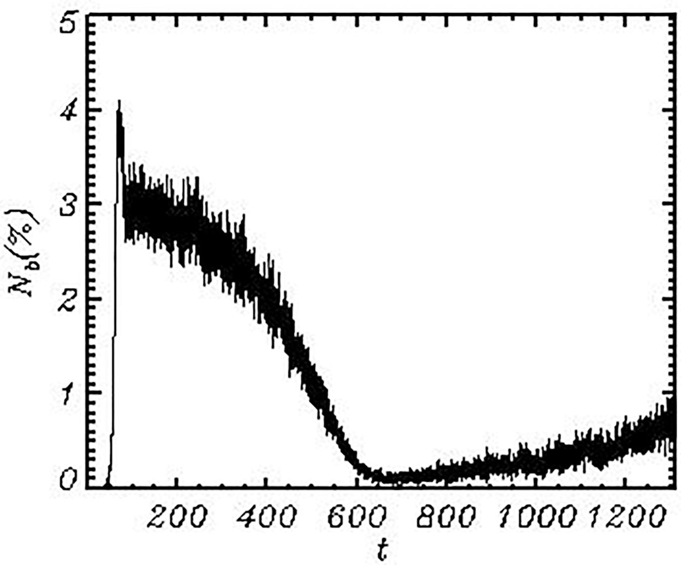
https://www.ocean-sci.net/14/453/2018/os-14-453-2018-f11

Figure 11Evolution of a number of the wave breaking events N_b expressed in percentage of the number of grid points N_x×N_y.

Download

The value of fetch in a periodic problem can be calculated by integration of a peak phase velocity $c_{p} = {|k|}^{- 1 / 2}$ over time.

\begin{matrix} (38) & F = \int_{t_{0}}^{t} c_{p} d t \end{matrix}

The JONSWAP dependencies for the frequency of a spectral peak ω_p and the full energy E are shown in Fig. 14 by thin curves. Dependence $ω_{p} \sim F^{1 / 3}$ is qualitatively valid. A dependence of the total energy on fetch does not look like a linear one, but it is worth noting that the JONSWAP dependence is evidently inapplicable to a very small and large fetch.

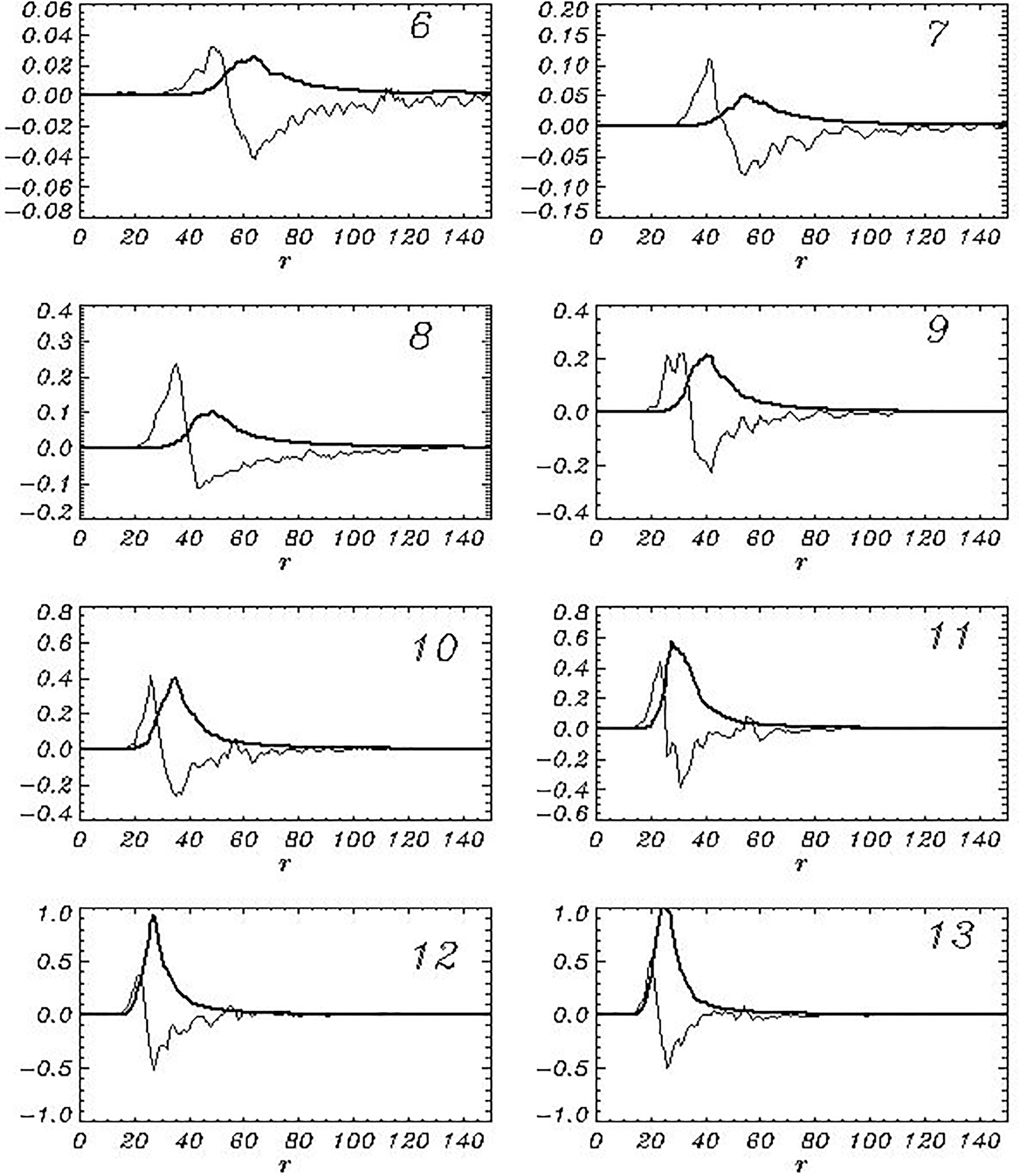
https://www.ocean-sci.net/14/453/2018/os-14-453-2018-f12

Figure 12Sequence of wave spectra S_h(r) (thick curves) and a nonlinear input term N(r) (thin curves) averaged over the eight consequent intervals of length Δt=100 starting from the sixth period.

Download

https://www.ocean-sci.net/14/453/2018/os-14-453-2018-f13

Figure 13Time evolution of the ratio E_l∕E_k.

Download

https://www.ocean-sci.net/14/453/2018/os-14-453-2018-f14

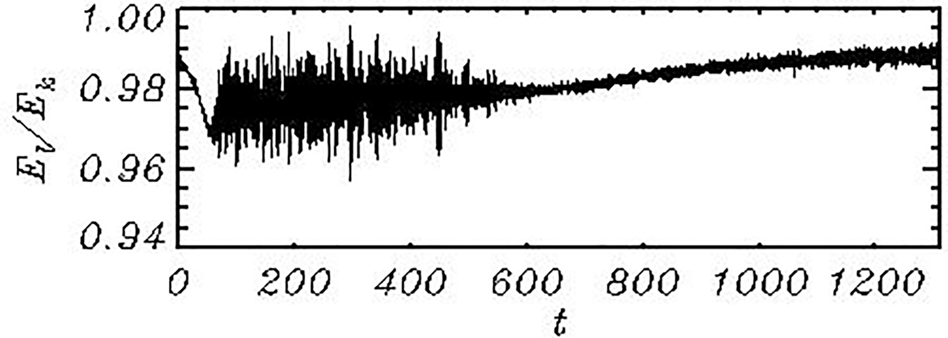
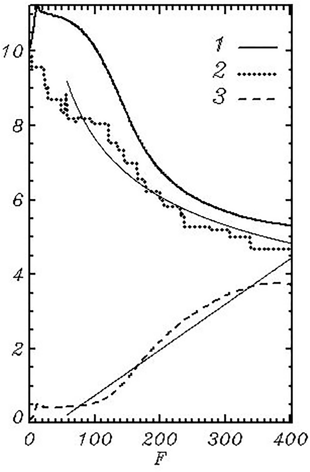
Figure 14Time evolution of weighted frequency ω_w (1) (Eq. 34), the spectral peak frequency $ω_{p} = k_{p}^{1 / 2}$ (2) and full energy E(3) (Eq. 28). Thin curves correspond to the empirical dependences for the peak wave number and energy. F is a distance passed by the spectral peak.

Download

5 Discussion

A model based on the full three-dimensional equations of a potential motion with a free surface was used for simulation of development of wave fields. The model is written in a surface-following nonstationary nonorthogonal coordinate system. The details of a numerical scheme and the results of the model validation were described in Chalikov et al. (2014). The main difference between the given model and HOS model (Ducroset et al., 2016) is that our model is based on a direct solution of the 3-D equations for the velocity potential. This approach is similar to that developed at the Technical University of Denmark (TUD; see Engsig-Karup et al., 2009). Actually, the models developed at TUD are targeted at the solution of a variety of problems including such problems as the modeling of wave interaction with submerged objects and the simulation of a wave regime in basins with real shape and topography.

In the current paper a three-dimensional model was used for simulation of the development of a wave field under the action of wind and dissipation. The input energy is described by a single term, i.e., surface pressure p in Eq. (4). It is traditionally assumed that the complex pressure amplitude in a Fourier space is linearly connected with the complex elevation amplitude through a complex coefficient called the β function. Such simple formulations can be imperfect. First, it is assumed that the wave field is represented by a superposition of linear modes with the slowly changing amplitudes and the phase velocity obeying a linear dispersive relation. This assumption is valid only for a low-frequency part of the spectrum. In reality, the amplitudes of the medium- and high-frequency modes undergo fluctuations created by reversible interactions. A solid dispersion relation does not connect their phase velocities with a wave number. In addition, it is also quite possible that a suggestion of the linearity of the connection between the pressure and elevation amplitudes is not precise, i.e., the β function can depend on the amplitudes of modes.

We are not familiar with any observational data that can be used for the formulation of a statistically provided scheme for calculation of the input energy to waves. The only method that can give more or less reliable results is the mathematical modeling of the statistical structure of a turbulent boundary layer above a curvilinear moving surface whose characteristics satisfy the kinematic conditions. The method described above is based on several millions of values of the pressure referred strictly to the surface. As a whole, the problem of a boundary layer seems even more complicated than the wave problem itself. Some early attempts to solve this problem were made on the basis of a finite-difference two-dimensional model of a boundary layer written in a simple surface following the coordinate (see review Chalikov, 1986). Waves were assigned as a superposition of linear modes with random phases, corresponding to the empirical wave spectrum. This approach was not quite accurate since it did not take into account the nonlinear properties of surface (for example, the sharpness of real waves and the absence of a dispersive relation for the waves of medium and high frequencies). The next step was the formulation of coupled models for a boundary layer and potential waves, both written in the conformal coordinates (Chalikov and Rainchik, 2010). The calculations showed that the pressure field consists mostly of random fluctuations not directly connected with the waves. A small part of these fluctuations are in phase with the surface disturbances. The calculated values of β in Eq. (13) have large dispersion. However, since the volume of data was very large, the shape of the β function was found with a high level of accuracy. Probably, the approximation of β used in the current work can be considered most adequate. We are planning additional investigations based on the coupled wind–wave models. The next step in the investigations of wave boundary layer (WBL) should use a three-dimensional LES approach. Note that even the availability of a large volume of data on the structure of WBL does not make the problem of parameterization of wind input in the spectral wave models easily solvable since the pressure is characterized by a broad continuous spectrum created by nonlinearity.

The wave breaking is obviously even more complicated than the input energy. Nevertheless, this problem can be simplified, if the common ideas used in the numerical fluid mechanics are accepted. For example, in the LES modeling a more or less artificial viscosity is introduced to prevent too large local velocity gradients. In fact the numerical instability terminating computations precedes the wave breaking. Hence, the scheme should prevent the breaking approach to preserve stability of the numerical scheme. Hence, a wave model should contain the algorithms preventing the appearance of too large slopes. A criterion of breaking is introduced not for recognizing the breaking itself, but for the choice of places where it might happen (or, unfortunately, might not happen). Finally, the algorithm should produce the local smoothing of elevation (and the surface potential). The algorithm should be highly selective so that the “breaking” could occur within narrow intervals and not affect the entire area. The exact criteria of the breaking events (most evident of them is the breaking itself) cannot be used for parameterization of breaking since in a coordinate system (1) the numerical instability occurs long before the breaking. In our opinion, the most sensitive parameter indicating potential instability is the curvilinearity (second derivative) of elevation.

In the current work, the breaking is parameterized by a diffusion algorithm with a nonlinear coefficient of diffusion providing high selectivity of the smoothing. We admit that such an approach can be realized in many different forms. The same situation is observed in a problem of the turbulence modeling for parameterization of subgrid scales. Note that the breaking dissipation in phase-resolving models is included in a more realistic manner than in spectral models. For example, the breaking is simulated in a physical space, which allows us to reduce the height and energy of the nonlinear waves composed of several modes. In spectral models the dissipation is distributed more or less arbitrarily over the entire spectrum. The spectral models sometimes include additional dissipation of short waves due to their modulation by long waves (Young and Babanin, 2006; Babanin et al., 2010). In the phase-resolving models this process has been included explicitly.

We can finally conclude that the physics included in wave models still rests on shaky ground. Nevertheless, the result of the calculations looks quite realistic, which convinces us that the approach deserves further development.

The numerical models of waves similar to that considered in this paper have a lot of important applications. First, they are a perfect tool for the development of physical parameterization schemes in spectral wave models. Second, a direct model can be used in future for the numerical simulation of wave processes in the basins of small and medium size. These investigations can be based on the HOS model (Ducrozet et al., 2016) or the model used in the current paper. However, the most universal approach seems to be developed at the Technical University of Denmark (see Engsig-Karup, 2009). Any model used for the long-term simulation of wave field evolution should include the algorithms describing transformation of energy similar to those considered in the current paper.

Data availability

The underlying data (150 Gb) are not publicly accessible. Any number of them can be shared upon request.

Competing interests

The authors declare that they have no conflict of interest.

Acknowledgements

The authors thank Olga Chalikova for her assistance in preparation of the paper as well as the anonymous reviewers for their constructive comments. This investigation was supported by Russian Science Foundation, project 16-17-00124.

Edited by: Neil Wells
Reviewed by: two anonymous referees

References

Alberello, A., Chabchoub, A., Monty, J. P., Nelli, F., Lee, J. H., Elsnab, J., and Toffoli, A.: An experimental comparison of velocities underneath focused breaking waves, Ocean Eng., 155, 201–210 2018.

Alves, J. H. G. M. and Banner, M. L.: Performance of a Saturation-Based Dissipation-Rate Source Term in Modeling the Fetch-Limited Evolution of Wind Waves, J. Phys. Oceanogr., 33, 1274–1298, 2003.

Al'Zanaidi, M. A. and Hui, H. W: Turbulent airflow over water waves-a numerical study, J. Fluid Mech., 148, 225–246, 1984.

Babanin, A. V., Tsagareli, K. N., Young, I. R., and Walker, D. J.: Numerical Investigation of Spectral Evolution of Wind Waves. Part II: Dissipation Term and Evolution Tests, J. of Phys. Oceanography, 40, 667–683, 2010.

Babanin, A. V.: Breaking and Dissipation of Ocean Surface Waves, Cambridge University Press, The Edinburgh Building, Cambridge, UK, 480 pp., 2011.

Beale, J. T.: A convergent boundary integral method for three-dimensional water waves, Math. Comput., 70, 977–1029, 2001.

Bonnefoy, F., Ducrozet, G., Le Touzé, D., and Ferrant, P.: Time-domain simulation of nonlinear water waves using spectral methods, in: Advances in Numerical Simulation of Nonlinear Water Waves, Advances in Coastal and Ocean Engineering, World Scientific, 11, 129–164, https://doi.org/10.1142/9789812836502_0004, 2010.

Causon, D. M., Mingham, C. G., and Qian, L.: Developments In Multi-Fluid Finite Volume Free Surface Capturing Methods, Advances in Numerical Simulation of Nonlinear Water Waves, 11, 397–427, 2010.

Chalikov, D.: The Parameterization of the Wave Boundary Layer, J. Phys. Oceanogr., 25, 1335–1349, 1995.

Chalikov, D.: Statistical properties of nonlinear one-dimensional wave fields, Nonlinear Proc. Geoph., 12, 1–19, 2005.

Chalikov, D.: Freak waves: their occurrence and probability, Phys. Fluids, 21, 076602, https://doi.org/10.1063/1.3175713, 2009.

Chalikov, D.: Numerical modeling of sea waves, Springer International Publishing AG, Switzerland, 330 pp., https://doi.org/10.1007/978-3-319-32916-1, 2016.

Chalikov, D. V.: Numerical simulation of windwave interaction, J. Fluid. Mech., 87, 561–582, 1978.

Chalikov, D. V.: Numerical simulation of the boundary layer above waves, Bound. Layer Met., 34, 63–98, 1986.

Chalikov, D. and Babanin, A. V.: Simulation of Wave Breaking in One-Dimensional Spectral Environment, J. Phys. Oceanogr., 42, 1745–1761, 2012.

Chalikov, D. and Babanin, A. V.: Simulation of one-dimensional evolution of wind waves in a deep water, Phys. Fluids, 26, 096607, https://doi.org/10.1063/1.4896378, 2014.

Chalikov, D. and Babanin, A. V.: Nonlinear sharpening during superposition of surface waves, Ocean Dynam., 66, 931–937, 2016a.

Chalikov, D. and Babanin, A. V.: Comparison of linear and nonlinear extreme wave statistics, Acta Oceanol. Sin., 35, 99–105, https://doi.org/10.1007/s13131-016-0862-5, 2016b.

Chalikov, D. and Makin, V.: Models of the wave boundary layer, Bound. Layer Met., 56, 83–99, 1991.

Chalikov, D. and Belevich, M.: One-dimensional theory of the wave boundary layer, Bound. Layer Met., 63, 65–96, 1992.

Chalikov, D. and Rainchik, S.: Coupled Numerical Modelling of Wind and Waves and the Theory of the Wave Boundary Layer, Bound. Layer Met., 138, 1–41, https://doi.org/10.1007/s10546-010-9543-7, 2010.

Chalikov, D. and Sheinin, D.: Direct Modeling of One-dimensional Nonlinear Potential Waves. Nonlinear Ocean Waves, edited by: Perrie, W., Adv. Fluid Mech. Ser., 17, 207–258, 1998.

Chalikov, D., Babanin, A. V., and Sanina, E.: Numerical Modeling of Three-Dimensional Fully Nonlinear Potential Periodic Waves, Ocean. dynam., 64, 1469–1486, 2014.

Clamond, D. and Grue, J.: A fast method for fully nonlinear water wave dynamics, J. Fluid Mech. 447, 337–355, 2001.

Clamond, D., Fructus, D., Grue, J., and Krisitiansen, O.: An efficient method for three-dimensional surface wave simulations. Part II: Generation and absorption, J. Comp. Physics, 205, 686–705, 2005.

Clamond, D., Francius, M,. Grue, J., and Kharif, C: Long time interaction of envelope solitons and freak wave formations, Eur. J. Mech. B.-Fluid., 25, 536–553, 2006.

Craig, W. and Sulem C.: Numerical simulation of gravity waves, J. Comput. Phys., 108, 73–83, 1993.

Dalrymple, R. A., Gómez-Gesteira, M., Rogers, B. D., Panizzo, A., Zou, S., Crespo, A. J., Cuomo, G., and Narayanaswamy, M.: Smoothed Particle Hydrodynamics For Water Waves, Advances in Numerical Simulation of Nonlinear Water Waves, 465–495, 2010.

Dommermuth, D. and Yue, D.: A high-order spectral method for the study of nonlinear gravity Waves, J. Fluid Mech., 184, 267–288, 1987.

Donelan, M. A., Babanin, A. V., Young, I. R., Banner, M. L., and McCormick, C.: Wave follower field measurements of the wind input spectral function. Part I. Measurements and calibrations, J. Atmos. Ocean Tech., 22, 799–813, 2005.

Donelan, M. A., Babanin, A. V., Young, I. R., and Banner, M. L.: Wave follower field measurements of the wind input spectral function. Part II. Parameterization of the wind input, J. Phys. Oceanogr., 36, 1672–1688, 2006.

Dysthe, K. B.: Note on a modification to the nonlinear Schrödinger equation for application to deep water waves, Proc. R. Soc. Lond. A, 369, 105–114, 1979.

Ducrozet, G., Bonnefoy, F., Le Touzé, D., and Ferrant, P.: 3-D HOS simulations of extreme waves in open seas, Nat. Hazards Earth Syst. Sci., 7, 109–122, https://doi.org/10.5194/nhess-7-109-2007, 2007.

Ducrozet, G., Bingham, H. B., Engsig-Karup, A. P., Bonnefoy, F., and Ferrant, P.: A comparative study of two fast nonlinear free-surface water wave models, Int. J. Numer. Meth. Fluids, 69, 1818–1834, 2012.

Ducrozet, G., Bonnefoy, F., Le Touzé, D., and Ferrant, P.: HOS-ocean: Open-source solver for nonlinear waves in open ocean based on High-Order Spectral method, Comp. Phys. Comm., 203, 245–254, https://doi.org/10.1016/j.cpc.2016.02.017, 2016.

Engsig-Karup, A. P., Harry, B., Bingham, H. B., and Lindberg, O.: An efficient flexible-order model for 3D nonlinear water waves, J. Comput. Phys., 228, 2100–2118, 2009.

Engsig-Karup, A., Madsen, M., and Glimberg, S. A.: massively parallel GPU-accelerated mode for analysis of fully nonlinear free surface waves, Int. J. Numer. Meth. Fl., 70, 20–36, 2675, https://doi.org/10.1002/fld.2675, 2012.

Fochesato, C., Dias, F., and Grilli, S.: Wave energy focusing in a three-dimensional numerical wave tank, Proc. R. Soc. A, 462, 2715–2735, 2006.

Fructus, D., Clamond, D., Grue, J., and Kristiansen, Ø.: An efficient model for three-dimensional surface wave simulations. Part I: Free space problems, J. Comput. Phys., 205, 665–68, 2005.

Gent, P. R. and Taylor, P. A.: A numerical model of the air flow above water waves, J. Fluid Mech., 77, 105–128, 1976.

Gou, Y., Teng, B., and Yoshida, S.: An Extremely Efficient Boundary Element Method for Wave Interaction with Long Cylindrical Structures Based on Free-Surface Green's function, Computation, 4, 36, 2016.

Greaves, D.: Application Of The Finite Volume Method To The Simulation Of Nonlinear Water Waves, Advances in Numerical Simulation of Nonlinear Water Waves, 11, 357–396, 2010.

Grilli, S., Guyenne, P., and Dias, F.: A fully nonlinear model for three-dimensional overturning waves over arbitrary bottom, Int. J. Num. Methods Fluids, 35, 829–867, 2001.

Grue, J. and Fructus, D.: Model For Fully Nonlinear Ocean Wave Simulations Derived Using Fourier Inversion Of Integral Equations In 3D, Advances in Numerical Simulation of Nonlinear Water Waves, 11, 1–42, 2010.

Guyenne, P. and Grilli, S. T.: Numerical study of three-dimensional overturning waves in shallow water, J. Fluid Mech., 547, 361–388, 2006.

Hasselmann, K.: On the non-linear energy transfer in a gravity wave spectrum, Part 1, J. Fluid Mech., 12, 481–500, 1962.

Hasselmann, D. and Bösenberg, J. : Field measurements of wave-induced pressure over wind-sea and swell, J. Fluid Mech., 230, 391–428, 1991.

Hasselmann, K., Barnett, T. P., Bouws, E., Carlson, H., Cartwright, D. E., Enke, K., Ewing, J. A., Gienapp, H., Hasselmann, D. E., Kruseman, P., Meerburg, A., Muller, P., Olbers, D. J., Richter, K., Sell, W., and Walden H.: Measurements of wind-wave growth and swell decay during the Joint Sea Wave Project (JONSWAP), Tsch. Hydrogh. Z. Suppl, A8, 1–95, 1973.

Hasselmann, S., Hasselmann, K., Allender, J. H., and Barnett, T. P.: Computations and Parameterizations of the Nonlinear Energy Transfer in a Gravity-Wave Specturm. Part II: Parameterizations of the Nonlinear Energy Transfer for Application in Wave Models, J. Phys. Oceanogr., 15, 1378–1392, 1985.

Hsiao, S. V. and Shemdin, O. H.: Measurements of wind velocity and pressure with a wave follower during MARSEN, J. Geophys. Res., 88, 9841–9849, 1983.

Iafrati, A.: Numerical Study of the Effects of the Breaking Intensity on Wave Breaking Flows, J. Fluid Mech., 622, 371–411, 2009.

Issa, R., Violeau, D., Lee E.-S., and Flament, H.: Modelling nonlinear water waves with RANS and LES SPH models, Advances in Numerical Simulation of Nonlinear Water Waves, 11, 497–537, 2010.

Kim, K. S., Kim, M. H., and Park, J. C.: Development of MPS (Moving Particle Simulation) method for Multi-liquid-layer Sloshing, Math. Probl. Eng., 2014, 350165, https://doi.org/10.1155/2014/350165, 2014.

Liu, Y., Gou, Y., Bin Teng, B., and Shigeo Yoshida, S.: An Extremely Efficient Boundary Element Method for Wave Interaction with Long Cylindrical Structures Based on Free-Surface Green's Function, Computation, 4, 36, https://doi.org/10.3390/computation4030036, 2016.

Lubin, P. and Caltagirone, J.-P.: Large eddy simulation of the hydrodynamics generated by breaking waves, Advances in Numerical Simulation of Nonlinear Water Waves, 11, 575–604, 2010.

Ma, Q. W. and Yan, S.: Qale-FEM method and its application to the simulation of free responses of floating bodies and overturning waves, Advances in Numerical Simulation of Nonlinear Water Waves, 165–202, 2010.

Miles, J. W.: On the generation of surface waves by shear flows, J. Fluid Mech., 3, 11, 02, https://doi.org/10.1017/S0022112057000567, 1957.

Rogers, W. E., Babanin, A. V., and Wang, D. W.: Observation-consistent input and whitecapping-dissipation in a model for wind-generated surface waves: Description and simple calculations, J. Atmos. Ocean. Tech., 29, 1329–1346, 2012.

Snyder, R. L., Dobson, F. W., Elliott, J. A., and Long, R. B.: Array measurements of atmospheric pressure fluctuations above surface gravity waves, J. Fluid Mech., 102, 1–59, 1981.

Tanaka, M.: Verification of Hasselmann's energy transfer among surface gravity waves by direct numerical simulations of primitive equations, J. Fluid Mech., 444, 199–221, 2001.

Ting C.-H, Babanin, A. V., Chalikov, D., and Hsu, T.-W.: Dependence of drag coefficient on the directional spreading of ocean waves, J. Geophys. Res., 117, C00J14, https://doi.org/10.1029/2012JC007920, 2012.

Toffoli, A., Onorato, M., Bitner-Gregersen, E., and Monbaliu J.: Development of a bimodal structure in ocean wave spectra, J. Geophys. Res., 115, C03006, https://doi.org/10.1029/2009JC005495, 2010.

Tolman, H. and Chalikov, D.: On the source terms in a third-generation wind wave model, J. Phys. Oceanogr., 26, 2497–2518, 1996.

Tolman, H. L. and the WAVEWATCH III ^∘R Development Group: User manual and system documentation of WAVEWATCH III ^∘R version 4.18 Environmental Modeling Center Marine Modeling and Analysis Branch, Contribution No. 316, 2014.

Touboul, J. and Kharif, C.: Two-Dimensional Direct Numerical Simulations Of The Dynamics Of Rogue Waves Under Wind Action, Advances in Numerical Simulation of Nonlinear Water Waves, 11, 43–74, 2010.

West, B., Brueckner, K., Janda, R., Milder, M., and Milton, R.: A new numerical method for surface hydrodynamics, J. Geophys. Res., 92, 11803–11824, 1987.

Young, I. R. and Babanin, A. V.: Spectral Distribution of Energy Dissipation of Wind-Generated Waves due to Dominant Wave Breaking, J. Phys. Oceanogr., 36, 376–394, 2006.

Young, D.-L., Wu, N.-J., and Tsay, T.-K.: Method Of Fundamental Solutions For Fully Nonlinear Water Waves, Advances in Numerical Simulation of Nonlinear Water Waves, 325–355, 2010.

Xue, M., Xu, H., Liu, Y., and Yue, D. K. P.: Computations of fully nonlinear three-dimensional wave and wave–body interactions. I. Dynamics of steep three-dimensional waves, J. Fluid Mech., 438, 11, 11–39, 2001.

Zakharov, V. E.: Stability of periodic waves of finite amplitude on the surface of deep fluid, J. Appl. Mech. Tech. Phys. JETF, 2, 190–194, 1968 (in English).

Zhao, X., Liu, B.-J., Liang, S.-X., and Sun, Z.-C.: Constrained Interpolation Profile (CIP) method and its application, Chuan Bo Li Xue/Journal of Ship Mechanics, 20, 393–402, https://doi.org/10.3969/j.issn.1007-7294.2016.04.002, 2016.

The wave spectrum looks more like the Sagrada Família (Gaudí) in Barcelona than the St Mary Axe (“The Gherkin”) in London.

The 2-D Fourier spectral “tail” looks like a peacock tail.

Articles

Short summary

Waves obtain energy from wind; they grow and increase in size and speed of propagation. The structure of wave fields becomes complicated due to appearance of new wave components. Finally, the sea surface looks like a poorly organized motion consisting of quickly running large hills and hollows covered with smaller waves. This process can be successfully simulated on computers. Such investigations allow us to understand the physics of sea waves, which is important for practice.