the Creative Commons Attribution 4.0 License.
the Creative Commons Attribution 4.0 License.
 | 22 Jun 2018
Acoustic mapping of mixed layer depth
Christian Stranne
Larry Mayer
Martin Jakobsson
Elizabeth Weidner
Kevin Jerram
Thomas C. Weber
Leif G. Anderson
Johan Nilsson
Göran Björk
Katarina Gårdfeldt
The ocean surface mixed layer is a nearly universal feature of the world oceans. Variations in the depth of the mixed layer (MLD) influences the exchange of heat, fresh water (through evaporation), and gases between the atmosphere and the ocean and constitutes one of the major factors controlling ocean primary production as it affects the vertical distribution of biological and chemical components in near-surface waters. Direct observations of the MLD are traditionally made by means of conductivity, temperature, and depth (CTD) casts. However, CTD instrument deployment limits the observation of temporal and spatial variability in the MLD. Here, we present an alternative method in which acoustic mapping of the MLD is done remotely by means of commercially available ship-mounted echo sounders. The method is shown to be highly accurate when the MLD is well defined and biological scattering does not dominate the acoustic returns. These prerequisites are often met in the open ocean and it is shown that the method is successful in 95 % of data collected in the central Arctic Ocean. The primary advantages of acoustically mapping the MLD over CTD measurements are (1) considerably higher temporal and horizontal resolutions and (2) potentially larger spatial coverage.
- Article
(8752 KB) -
Supplement
(633 KB) - BibTeX
- EndNote


The surface mixed layer is an important and nearly universal feature of the world oceans. It is defined as a quasi-homogeneous layer that extends from the surface down to the penetration depth of turbulent mixing, generated by wind stress and buoyancy fluxes at the air–sea interface (Kraus and Turner, 1967; Price et al., 1986). The MLD is an important parameter within several atmospheric and oceanographic research disciplines as the transfer of mass, momentum, and buoyancy across the mixed layer provides the source of almost all oceanic motions (de Boyer Montégut et al., 2004). Variations in MLD influence air–sea interactions through the storage of various gases, such as carbon dioxide and methane (Kraus and Businger, 1994). The MLD also affects the vertical distributions of dissolved and particulate biological and chemical components in surface waters (Gardner et al., 1995) and is thus one of the main factors controlling primary production (Behrenfeld and Falkowski, 1997; Sverdrup, 1953). The surface mixed layer is also of importance since it represents a reservoir for pollutants that are deposited from the atmosphere and cycled between the atmosphere and the surface waters (Nerentorp Mastromonaco et al., 2017). Furthermore, temporal and spatial variability in the MLD is essential for validating and improving mixed layer parameterizations (Ling et al., 2015; Martin, 1985; Noh et al., 2002) and as diagnostics in mixed layer budgets (Hasson et al., 2013; Montégut et al., 2007). The properties, depth, and behavior of the surface mixed layer also play an important role in understanding acoustic propagation in the ocean.
The MLD is controlled primarily by surface stress (exerted by wind or sea ice), buoyancy fluxes (heating–cooling, ice melt–formation, lateral advection, or precipitation–evaporation), and dissipation (Large et al., 1994; Timmermans et al., 2012). Thus, any variation in the MLD can be linked to these processes. It is well established that the MLD varies on diurnal to inter-decadal timescales (Bissett et al., 1994; Kara et al., 2003; Li et al., 2005; Polovina et al., 1995), but higher-frequency variability is poorly understood due to observational limitations. For direct measurements of the MLD, various forms of conductivity, temperature, and depth (CTD) sensor data are collected from ships, moorings, or gliders. These collect discrete profiles through the water column with a frequency of typically less than one profile per 10 min. Broad global coverage of the distribution of the MLD is becoming increasingly available through salinity and temperature stratification data from the ARGO float program (Freeland et al., 2010), but the high spatial frequency of ocean thermohaline variability is still strongly undersampled (Guinehut et al., 2012). Satellite-derived products provide global synoptic coverage of, for example, sea level (MacIntosh et al., 2016), sea surface temperature (Donlon et al., 2010), and sea surface salinity (Font et al., 2013; Lagerloef et al., 2012) but are essentially restricted to near-sea-surface properties.
Since the early 20th century, active acoustic sensors have been used to track military targets in the water column (MacLennan and Simmonds, 2013). Not long after the first military applications, acoustic water column mapping with echo sounders was applied to fisheries science, for which the detection and quantification of fish distributions were the primary focus (Kimura, 1929; MacLennan, 1990). The applications of acoustic water column mapping have broadened in recent years to include marine ecosystem acoustics (Benoit-Bird and Lawson, 2016; Godø et al., 2014), observations of gas bubbles and oil droplets associated with natural seeps (Jerram et al., 2015; Merewether et al., 1985), and fossil fuel production (Hickman et al., 2012; Weber et al., 2012). Acoustic imaging of the water column has also been used within the field of physical oceanography; single-beam echo sounders can capture fine-scale oceanographic structures typically attributed to biological scattering or turbulent microstructures (Klymak and Moum, 2003; Pingree and Mardell, 1985; Trevorrow, 1998). Larger-scale thermohaline structures have been observed with lower-frequency seismic systems (e.g., Holbrook et al., 2003). Custom-built echo sounders utilizing wideband frequency-modulated pulses have been deployed since the 1970s (e.g., Holliday, 1972), but have received renewed attention as they have become commercially available (Duda et al., 2016; Lavery et al., 2010; Stranne et al., 2017). The advantages of wideband echo sounders, compared to conventional narrowband systems, include increased signal-to-noise ratio (SNR), increased range resolution through pulse-compression processing (Stanton and Chu, 2008; Turin, 1960), and the ability to study the frequency response of individual targets (Lavery et al., 2010; Stanton et al., 2010).
The increased SNRs of wideband echo sounders have made it possible to map density stratification in the ocean. Stranne et al. (2017) were able to acoustically image individual thermohaline steps resulting from the intrusion of warm and salty Atlantic waters into the colder and less saline Arctic waters. The range resolution provided by the wideband sonar enabled the detection of individual density layers separated by less than 0.5 m to depths of about 300 m. These thermohaline layers represent a change in temperature of typically 0.05 ∘C and a change in salinity of 0.015, with corresponding acoustic reflection coefficients at the layer interface as low as . Although the ensonified area (i.e., the region covered by the beam) is smaller at shallower depths for a downward-looking echo sounder (leading to a weaker scatter strength), this is compensated for by generally higher reflection coefficients at the base of the mixed layer, meaning that the MLD is more readily detectable with wideband echo sounders. Here we show that underway profiling using wideband echo sounding systems at up to several pings per second can map the behavior of the MLD at very high spatial resolution.
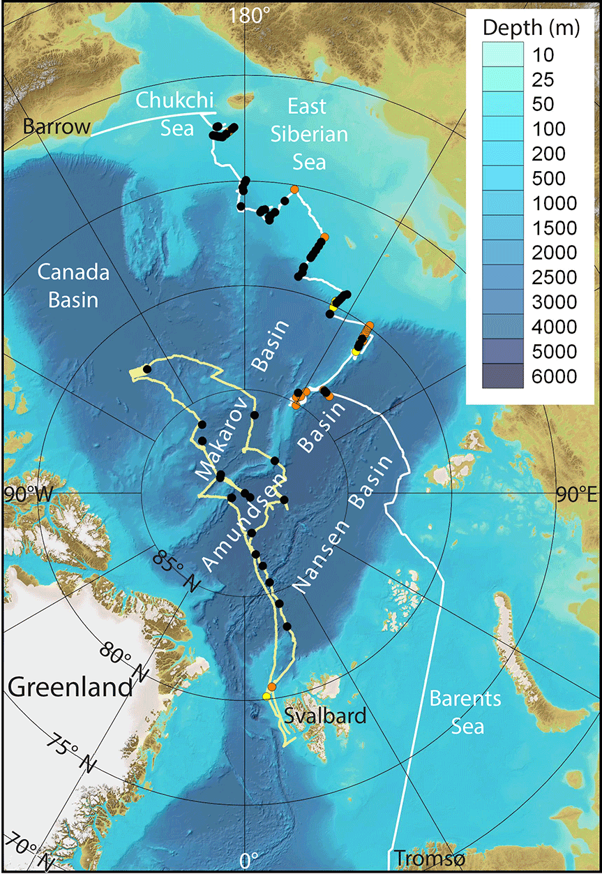
Figure 1Map showing cruise tracks for the SWERUS-C3 cruise (white) and the Arctic Ocean 2016 cruise (yellow). CTD stations are shown as dots; black indicates the MLD was successfully observed acoustically, red indicates the MLD was not successfully observed acoustically, and yellow indicates no mixed layer was present.
2.1 Data and the regional setting
Acoustic water column data were collected throughout the Arctic Ocean during two expeditions with Swedish Icebreaker (IB) Oden: Leg 2 of the Swedish–Russian–US Arctic Ocean Investigation of Climate–Cryosphere–Carbon Interactions 2014 Expedition (SWERUS-C3) and the Arctic Ocean 2016 Expedition (AO2016).
Leg 2 of SWERUS-C3 departed on 20 August 2014 from Barrow, Alaska, and ended on 4 October in Tromsø, Norway. The expedition covered mainly the shallow areas of the East Siberian Sea continental shelf and shelf slope (Fig. 1). The median water depth of the 78 CTD stations investigated from SWERUS-C3 is 340 m. The hydrography of this area can be characterized as dynamic and seasonally variable as it is influenced by large river runoff, coastally trapped waves, ice formation and melting, and brine rejection in coastal polynyas.
The AO2016 expedition took place between 8 August and 19 September 2016, departing from and returning to Svalbard (Fig. 1). One specific research goal during AO2016 was dedicated to investigating the possibility to detect and map thermohaline stratification using a mid-water wideband echo sounder. The cruise track covered mainly the central Arctic Ocean and the median water depth of 24 CTD stations investigated is 4000 m (Fig. 1). Together, the SWERUS-C3 and AO2016 expeditions spanned much of the breadth and depth of the Arctic Ocean and provided wideband acoustic data in a variety of oceanographic settings.
2.2 Wideband water column acoustic data collection
The wideband water column backscatter data presented here were collected with a Simrad EK80 split-beam scientific echo sounder (SBES) installed on IB Oden. The system was operated continuously during both the SWERUS-C3 and AO2016 expeditions.
The SBES consisted of a Simrad EK80 wideband transceiver transmitting through a standard Simrad ES18-11 transducer installed in the “ice knife” near the bow of the vessel and protected by an ice window. This transducer model is widely installed in fishery research vessels, typically operating at 18 kHz with a −3 dB beamwidth of 11∘. In 2014, the transducer model was tested with a Simrad EK80 wideband transceiver and determined to have a useable two-way frequency response over 15–25 kHz. Thus, a frequency range of 15–25 kHz was used throughout the EK80 data collection period on IB Oden.
Transmit power was maintained at the maximum setting of 2000 W to compensate for losses through the ice protection window and improve signal-to-noise (SNR) characteristics, especially during noisy hull–ice interactions. Transmission pulse lengths were adjusted over a range of 1–8 ms in an effort to minimize the extent of autocorrelation sidelobes (sidelobes are typically minimized with shorter pulses) while maximizing the SNR (better with longer pulses). All EK80 operation was controlled and monitored around the clock using the Simrad user interface to adjust pulse length and range-recording duration. Data were logged in the Simrad .raw format.
Position and attitude information were provided to the echo sounder as an integrated solution by a Seapath Seatex 330 GPS/GLONASS navigation and motion reference system. Vessel motion was minimal (typically less than 1∘ pitch and roll in the data presented here) and thus does not appreciably affect the observations of horizontally oriented backscattering layers occupying broad portions of the beam.
During the AO2016 expedition, a small delay was applied to the EK80 transmit–receive cycle trigger in order to avoid transmission interference from the two other echo sounding systems (Kongsberg EM122 12 kHz multibeam and SBP120 2–7 kHz sub-bottom profiler) in the earliest portion of the EK80 receive cycle corresponding to the upper water column region of interest.
2.3 EK80 post-processing methodology
The dataset collected with the EK80 was match filtered with an ideal replica signal using a MATLAB software package provided by the system manufacturer, Kongsberg Maritime (Lars Anderson, personal communication, 2014). After match filtering, ship-related noise was found within the signal band. A band-pass filter with 16 and 22 kHz cutoff frequencies was applied to the data to exclude the noise.
Sound speed profiles were calculated from CTD-derived temperature, salinity, and pressure data using the International Thermodynamic Equation of Seawater (IOC, SCOR and IAPSO, 2010). Ranges from the transducer were then calculated using the cumulative travel times through sound speed profile layers based on the nearest (in time) CTD profile. These ranges were then converted to depths by compensating for the transducer location relative to the static waterline on IB Oden and the heave of the vessel.
2.4 EK80 extended target calibration procedure
The EK80 was calibrated onboard the Oden on 1 September 2015, following a standard method described by Demer et al. (2015). A 64 mm copper sphere of known acoustic properties was suspended on a monofilament line and moved through the SBES field of view. The calibration data were collected in relatively calm seas and atmospheric conditions while the Oden drifted. All propulsion systems were secured during the calibration procedure in order to reduce noise in the water column. A CTD profile was collected immediately before calibration operations.
Utilizing a calibration sphere target strength model based on the work by Faran (1951) and MacLennan (1981) (MATLAB software; Dezhang Chu, personal communication, 2015), a calibration offset (C=8.5 dB, averaged over the transducer beam width) was calculated using a temperature of 0 ∘C and a salinity of 34.5 at the sphere depth of approximately 80 m. This calibration offset represents the difference between the nominal target strength (TS) observed by the EK80, as predicted after match filtering, and the modeled TS of the calibration sphere. The offset is then applied to subsequent measurements of TS, yielding calibrated TS results for the EK80 datasets.
2.5 Estimates of the reflection coefficient from EK80 observations
The TS of an ideally smooth layer is a function of both the reflection coefficient (R) and the ensonified area (A). Here, we assume that A is limited by the width of the EK80 beam (rather than the length of the pulse) such that A can be estimated as
where φ is half the beam width and z is the depth in the sonar reference frame. Following Lurton and Leviandier (2010) the TS for a layer at depth z, with reflection coefficient R, can then be estimated as
For our estimates of observed R, we simply invert the above equation to solve for R:
where TS is the calibrated acoustic backscatter observation from the EK80.
2.6 CTD
CTD data were collected with a Sea-Bird 911 equipped with dual Sea-Bird temperature (SBE 3) and conductivity (SBE 04C) sensors. The CTD data files were post-processed with SBE Data Processing software, version 7.26.6 (available at http://www.seabird.com/software). The alignment parameter was tuned following the suggested method described in the SBE Data Processing manual (available at http://www.seabird.com/software). All CTD data presented are averaged in 10 cm vertical bins.
The reflection coefficient from CTD data (RCTD) was calculated through
where each element i has a corresponding depth z(i), the depth of RCTD(i) is the average of z(i−1) and z(i), and η is the acoustic impedance given by
where V is the sound speed and ρ the seawater density. The accuracies of the pressure, conductivity, and temperature sensors are 0.0015 %, 0.0003 S m−1, and 0.001 ∘C, respectively. All conversions (salinity, density, and sound speed) were made according to the International Thermodynamic Equation of Seawater (IOC, SCOR and IAPSO, 2010).
2.7 MLD derived from CTD
To determine the MLD, we apply the method presented in de Boyer Montégut et al. (2004) in which successively deeper data points in each of the CTD potential temperature profiles are examined until one is found with a potential temperature value differing from the value at the 10 m reference depth by more than the threshold value (ΔT) of ±0.2 ∘C. Using this approach, the MLD is then assumed to be at least 10 m deep, and any shallower well-mixed sections in the water column are not taken into consideration (de Boyer Montegut et al., 2004). The reference depth applied by de Boyer Montegut et al. (2004) was chosen to avoid the diurnal variability of the mixing layer (typically found at depths < 10 m) while keeping the longer-term variability of the mixed layer.
We investigated the shallow (< 50 m depth) EK80 water column data from approximately 1 h before to 1 h after the time of each CTD cast, for a total of 102 CTD stations throughout both expeditions (Fig. 1). An example of acoustic mapping of the MLD over a 117 km long cruise track (about 12 h) in the central Arctic Ocean is shown in Fig. 2.
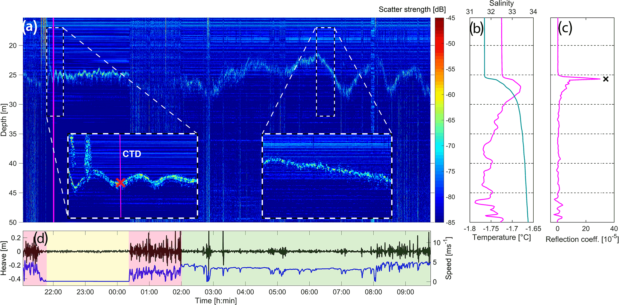
Figure 2Continuous tracking of MLD in the central Arctic Ocean over a 117 km cruise track. Data were acquired 12–13 September 2016 at 14.5∘ E, 86.1∘ N. (a) EK80 echogram (2 ms pulse length) with magnified insets (dashed boxes) showing the MLD while drifting (left) and while steaming (right). (b) CTD profiles showing temperature (magenta) and salinity (cyan). (c) Reflection coefficients derived from CTD data (magenta) and from scatter strength; black cross represents the observed scatter strength of −65 dB at this depth extracted from the left inset in (a). (d) Heave (black), speed over ground (blue), and time periods corresponding to ice breaking (red), steaming (green), and drifting (yellow). Vertical magenta lines in (a) show the position of the CTD. The red cross in (a) (left inset) marks the depth of the reflection coefficient spike in (c). Note that the ability to detect MLD acoustically is severely reduced while breaking ice.
Table 1Success and failure rates of acoustic detection of MLD when present in CTD data.
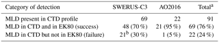
a Of the total 102 CTD stations investigated, 11 stations (9 in SWERUS-C3 and 2 in AO2016) did not have a well-defined MLD (yellow category in Fig. 1) and are not included in these statistics. An example of this category is shown in Fig. S1. b Of the 21 acoustic detection failures in the SWERUS-C3 data, more than half are related to the relatively deep ship draft of IB Oden and four are related to noise of unknown source that appeared in the EK80 data towards the end of the cruise. When not counting these particular modes of failure, which could possibly be addressed with different vessel parameters, the MLD acoustic detection success rate is close to 90 % in the SWERUS-C3 data.
We categorize CTD stations where EK80 data are available into three classes (Fig. 1): black indicates that a mixed layer is present in the CTD data and the MLD is visible in the EK80 data (success); red indicates that a mixed layer is present in the CTD data but the MLD is not visible in the EK80 data (failure); and yellow indicates that a mixed layer is not present in the CTD data. The classification is done subjectively by visual scrutiny of each echogram and subsequent comparison with CTD profiles; this process is meant to provide a general idea of how often a mixed layer is present in the in situ CTD data and the success rate of the remote EK80 MLD detection. In order to automate the EK80 MLD detection process, a stratification tracking tool needs to be produced. No such tool is available but methods used within the seismic processing or seismic oceanography fields can also likely be applied to sonar data.
Table 2Statistics for MLDEK80 and MLDCTD with the four outliers (Fig. 3) excluded; all units are meters.
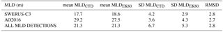
Of the 102 CTD stations investigated, a mixed layer is present in 91 CTD profiles (90 %); of these 91 confirmed MLD profiles, the MLD is simultaneously visible in the EK80 data in 69 instances (76 %; Table 1). The ΔT threshold estimate method yielded similar results to that of using acoustic data, with a root mean square deviation (RMSD) between the two methods of about 3 m (Table 2). The original ΔT threshold (0.2 ∘C) as presented in de Boyer Montégut et al. (2004) worked well for the SWERUS-C3 CTD stations but generally failed in the central Arctic Ocean due to the generally weaker density contrast at the base of the mixed layer (as shown in Fig. S3). Therefore, we used a modified ΔT threshold of 0.05 ∘C on CTD data from AO2016. Note that, even though instances in which the ΔT threshold method clearly fails are excluded in these statistics, there are still instances in which it provides less than ideal MLD estimates. The deviation therefore reflects inaccuracies in both methods. The CTD ΔT threshold method is constructed to avoid the mixing layer (i.e., shallower and generally weaker stratification that varies on a diurnal timescale, not to be confused with the mixed layer, which is the focus of this study). We note that the nice agreement between the acoustic method and the CTD ΔT threshold method implies that we are generally also catching the mixed layer with the acoustic method. The density threshold approach presented de Boyer Montégut et al. (2004) was tested with close to identical results. We opted to use and display the results from the temperature threshold method, as it is simpler and there are more temperature data available than there are salinity data (in, e.g., the World Ocean Database), thus rendering this method more useful in a general sense. Note that the same problems we had with the temperature threshold (we had to adjust it for the central Arctic Ocean) also showed up for the density threshold method.
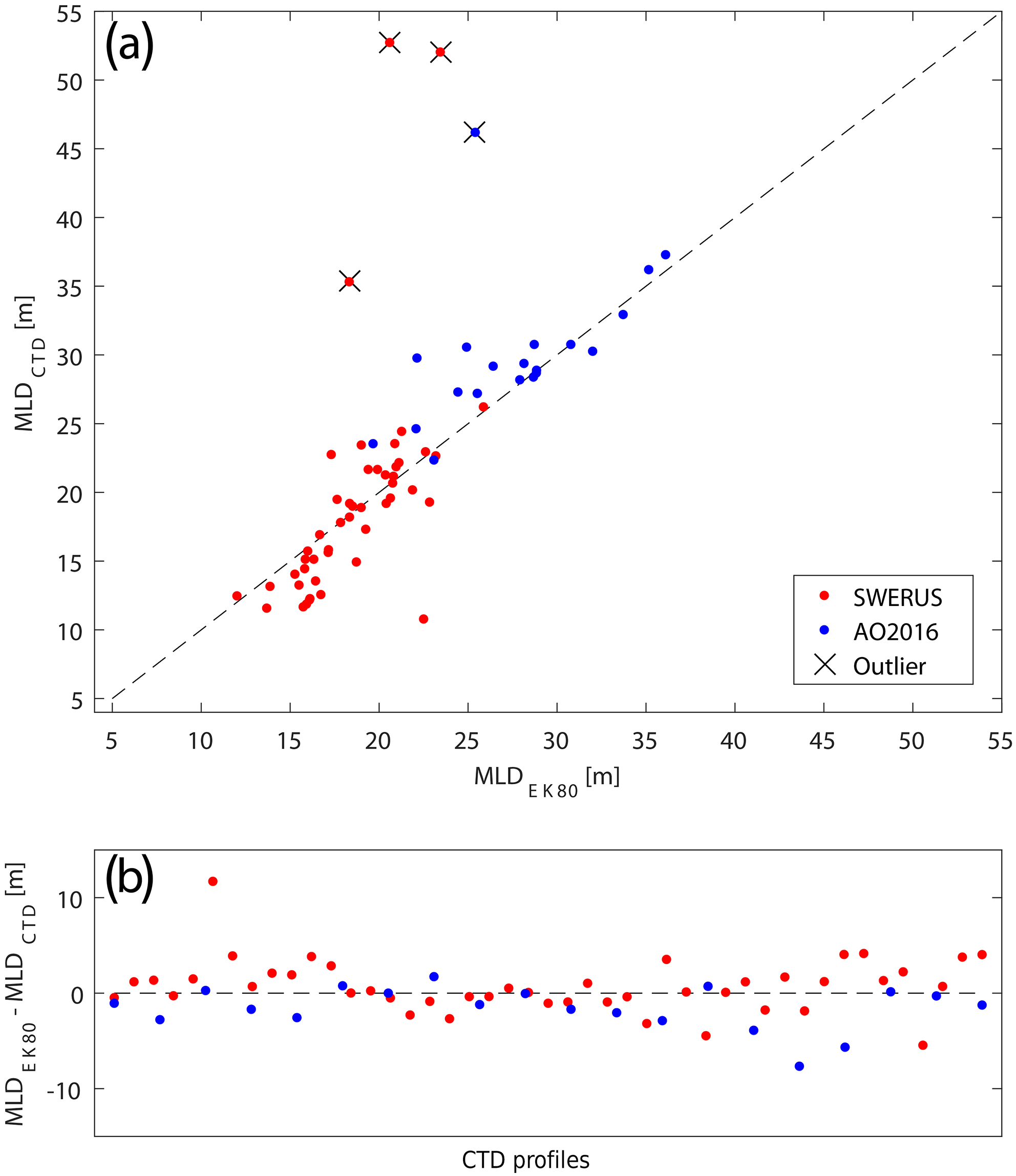
Figure 3(a) MLD for the individual stations derived from CTD (MLDCTD) vs. MLD derived from EK80 data (MLDEK80). (b) Difference between MLDEK80 and MLDCTD. In total, four outliers (black crosses in a) for which the ΔT threshold method fails (as exemplified in Fig. S2) are excluded from the statistics. Note that the original ΔT threshold (0.2 ∘C) as presented in de Boyer Montégut et al. (2004) generally failed in the central Arctic Ocean (Fig. S3) and that we instead used a modified ΔT threshold of 0.05 ∘C on CTD data from AO2016.
4.1 MLD observations
The typical summer MLD of the Arctic Ocean is ∼ 20 m (Steele et al., 2008). By applying a density threshold method for determining the MLD, Toole et al. (2010) reported for the central Canada Basin an average summer MLD of 16 m and an average winter MLD of 24 m. The shallower mean MLD in the SWERUS-C3 data is consistent with the large river runoff into the Siberian shelf seas, which should lead to a generally shallower mixed layer compared to the AO2016 data from the central parts of the Arctic Ocean (Large et al., 1994). Given the dynamic nature of the more coastal Leg 2 SWERUS-C3 cruise track compared to the open-ocean-dominated AO2016 cruise track, we were expecting larger MLD variability in the SWERUS-C3 data. We cannot see such a tendency in our data (Table 2), but again the basis of the statistics is rather poor.
In general, MLD variations between the different regions of the Arctic Ocean covered in this study match well with mean Arctic Ocean MLD based on other field observations (Ilıcak et al., 2016; Peralta-Ferriz and Woodgate, 2015), with shallow MLDs along the East Siberian Sea, slightly deeper MLDs in the Canada Basin, and the deepest MLDs in the central Arctic Ocean. As the emphasis of this paper is mainly on the acoustic method rather than the actual MLD observations, we are hesitant to draw any conclusions based on the MLD statistics presented in Table 2, especially when considering the small number of observations on which the statistics are based.
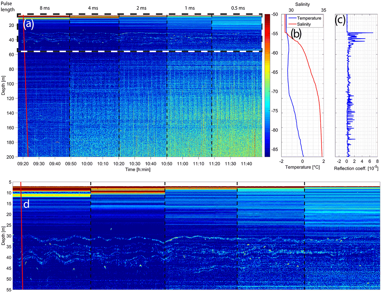
Figure 4Comparison of EK80 data with different pulse lengths. Data were acquired on 26 August 2016 at 140.6∘ W, 86.8∘ N. (a) EK80 echogram. (b) CTD profiles showing temperature (blue) and salinity (red). (c) Reflection coefficients derived from CTD data. (d) Enlargement of dashed box in (a). In (a) and (d), the vertical red line is the CTD position and the vertical dashed black lines indicate changes in pulse length (decreasing from 8 to 0.5 ms).

Figure 5Tendency of increased range resolution in EK80 data with smaller pulse length. Data were acquired on 29 August 2016 at 148.1∘ W, 86.1∘ N. (a) EK80 echogram with backscatter strength in dB on the color bar. (b) CTD profiles showing temperature (blue) and salinity (red). (c) Reflection coefficients derived from CTD data. Note that, as there is no ground-truth CTD cast within the later section of the echogram, there might be splitting and merging of layers (as shown in Stranne et al., 2017) and other changes in the stratification behavior occurring near the change in pulse length.
4.2 Sampling frequency
With the acoustic method we can observe the MLD at a horizontal resolution far exceeding alternative in situ methods, such as CTD profiles. The acoustic method enables the study of internal waves propagating on the layer interface at the base of the mixed layer (left inset, Fig. 2a). Internal waves are a ubiquitous phenomenon in the ocean and drive vertical mixing that is important for the global ocean circulation and primary production (Garret and Munk, 1979; Denman and Gargett, 1983; Munk and Wunsch, 1998). Stranne et al. (2017) observed internal waves that caused vertical undulations of the stratification down to depths of about 300 m. While these deeper internal waves were clearly not excited by the vessel, we cannot exclude the possibility that some of the vertical undulations of the MLD seen here are due to near-surface internal waves generated by the Oden (Nansen, 1905).
The recording duration of the EK80 was set to observe the full water column, resulting in a ping rate of around 0.1 ping s−1 when synchronized with the multibeam echo sounder in deep water (i.e., ping rate is limited by recording range on the outer swath, which can be more than twice the water depth). The ping rate can be set much higher (up to several pings per second) in shallow water or if only data from the shallow part of the water column are to be collected. In our data the MLD is clearly visible while drifting and steaming, but the quality of the data underway would benefit from a higher ping rate; specifically, the highest-frequency temporal and/or spatial variations in MLD are likely undersampled at this lower ping rate while the vessel is moving (right inset Fig. 2a).
4.3 Vertical detection limits
The cruise track of the SWERUS-C3 expedition during Leg 2 covers mainly the shallow areas of the East Siberian Sea shelf and shelf slope, an area that is heavily influenced by river runoff (e.g., from the Lena River). The freshwater input (or negative buoyancy flux) to the coastal waters leads to a generally shallower MLD (Large et al., 1994). This is clearly manifested in our data in which the average MLD from the shelf-dominated SWERUS-C3 cruise is approximately two-thirds that of the sea ice-covered, deep-basin-dominated AO2016 cruise (Table 2).
The deep depth limit for detecting ocean stratification with this particular EK80 setup appears to be around 300 m (Stranne et al., 2017), while the shallow depth limit depends on the draft of the hull-mounted transducer and the pulse length. On the Oden, the EK80 transducer is mounted at a draft of 7 m and, depending on pulse length, we generally observe useful data starting at 7.5–12 m of depth from the surface (0.5–5 m from the transducer; Fig. 4d). The amount of data lost at the upper boundary is reduced with shorter pulse length (Fig. 4d); these data also show the better range resolution obtained with a shorter pulse length (Fig. 5), but there is a serious trade-off in terms of reduced SNR (Fig. 4a). More data are needed in order to determine the optimal pulse length for EK80 MLD detection as it also depends on region and platform.
Due to ship draft and the data loss at very close range from the transducer, the shallow MLDs seen in some of the SWERUS-C3 CTD profiles are sometimes difficult to detect acoustically with the EK80 (Fig. S4). This is the most common factor explaining more than 50 % of the failures to acoustically detect the MLD during SWERUS-C3.
4.4 Biological scatter
In the example shown in Fig. 2, the reflections are likely stemming from the impedance contrast from the ocean stratification alone; this is supported by the close match between the theoretical reflection coefficient calculated from the CTD data and the reflection coefficient derived from the calibrated acoustic backscatter data. This agreement among reflection coefficients is consistent with observations of deeper thermohaline staircase stratification from the central Arctic Ocean presented in Stranne et al. (2017). In the SWERUS-C3 data, biological scatterers are generally identified at CTD stations closer to the coast. Biological scattering can potentially obscure the reflections from the MLD boundary (Fig. 6); at other times, the distribution of biological scatterers may coincide with the ocean stratification and enhance the layer reflections.
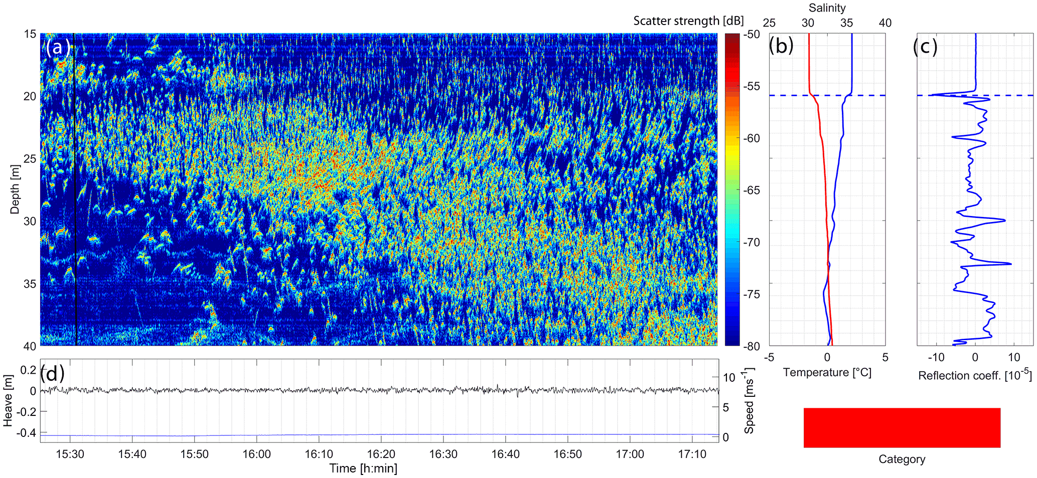
Figure 6MLD obscured by biological scatter. Data were acquired on 15 September 2014 at 143.2∘ E, 79.9∘ N. (a) EK80 echogram with black vertical line indicating the position of the CTD rosette. (b) CTD profiles showing temperature (blue) and salinity (red). (c) Reflection coefficients derived from CTD data. The horizontal dashed line in (b) and (c) show the MLD as defined by the ΔT threshold method. Also shown at the lower right is the category (red) of this particular CTD station, indicating the failure of the acoustic method to detect the MLD amidst strong biological scattering that spans across the MLD.
4.5 Further aspects
At the time of the SWERUS-C3 expedition, we did not yet realize that the EK80 was capable of MLD detection and accordingly nothing was done to optimize the performance of the EK80 to detect ocean stratification in 2014. At four of the SWERUS-C3 CTD stations, the MLD is obscured by noise from an unknown source (Fig. S5) but the source was not identified and no actions were taken to reduce it. This type of noise did not occur in the acoustic data from the later AO2016 cruise.
In this study we show that the MLD can be tracked acoustically with high horizontal and vertical resolutions over large distances (Fig. 2). The method is better suited for MLD tracking in the open ocean, where it was successfully detected at 95 % of the ground-truth CTD stations, compared to coastal areas where the success rate was 70 %. The lower success rate in coastal areas is partly related to the greater abundance of biological scatterers, but in this case more importantly to the generally shallower MLDs, which were sometimes impossible to detect acoustically due to IB Oden's vessel draft of 7 m and data loss close to the transducer. Smaller coastal vessels with shallower draft may be better suited to acoustically track the MLD in these regions.
The acoustic method of determining MLD yields results similar to the established ΔT threshold method with a root mean square deviation of about 3 m. There are large uncertainties associated with the ΔT threshold method and the MLDEK80 estimates should likely provide better precision, at least under some circumstances, as exemplified in Fig. S2.
While the MLD is a crucial component within the Arctic Ocean in terms of physical, chemical, and biological processes (Peralta-Ferriz and Woodgate, 2015), the discrepancy between observed and modeled MLDs in the Arctic can be quite significant (Ilıcak et al., 2016). The method of observing the MLD remotely, by means of ship-mounted echo sounders, allows for larger and more efficient observational coverage. It should be noted, however, that the acoustic method cannot completely replace in situ measurements (partly because of the need for ground-truthing the acoustic data), but rather it presents a powerful complementary method to “connect the dots” at high resolution between CTD stations.
Methods of utilizing ocean reflectivity from multichannel seismic systems to reconstruct temperature and salinity stratification between CTD casts have been investigated (Biescas et al., 2014; Papenberg et al., 2010; Wood et al., 2008). The increased vertical resolution (from ∼ 10 m with multichannel seismic data to < 0.5 m with wideband acoustics; Stranne et al., 2017) facilitates the detection of much finer thermohaline structures in the water column, including the MLD, and can potentially vastly improve these methods.
Many vessels are equipped with underway sonar systems, and thus the method presented here is a step toward collecting large amounts of ocean stratification data globally. Such large-scale acoustically obtained stratification data can become a fundamental link tying discrete ARGO float profiles (Freeland et al., 2010) with large-scale synoptic coverage of sea surface temperature and salinity data derived from satellites (Font et al., 2013; Lagerloef et al., 2012). Furthermore, modeling approaches for estimating MLD are often based on remote sensing data, including lidar data for scattering layers and satellite data for sea surface salinity, sea surface temperature, surface wind speed, and sea level (Ali and Sharma, 1994; Durand et al., 2003; Hoge et al., 1988; Yan et al., 1990). High-resolution acoustic mapping of the MLD will add important inputs to these models.
All data supporting the figures and text in this paper are available upon request from the corresponding author.
The supplement related to this article is available online at: https://doi.org/10.5194/os-14-503-2018-supplement.
The authors declare that they have no conflict of interest.
We thank the crew of the IB Oden and the Swedish Polar Research
Secretariat for their support. Christian Stranne and Martin Jakobsson received
support from the Swedish Research Council (Vetenskapsrådet, 2014-478 and
2016-04021). Larry Mayer, Elizabeth Weidner, Kevin Jerram, and Thomas C. Weber
acknowledge the support of NOAA grant NA15NOS400002000 and NSF grant 1417789.
Johan Nilsson received support from the Swedish National Space
Board.
Edited by: Neil
Wells
Reviewed by: two anonymous referees
Ali, M. M. and Sharma, R.: Estimation of mixed layer depth in the equatorial Indian Ocean using Geosat altimeter data, Marine Geodesy, 17, 63–72, https://doi.org/10.1080/15210609409379710, 1994.
Behrenfeld, M. J. and Falkowski, P. G.: Photosynthetic rates derived from satellite-based chlorophyll concentration, Limnol. Oceanogr., 42, 1–20, https://doi.org/10.4319/lo.1997.42.1.0001, 1997.
Benoit-Bird, K. J. and Lawson, G. L.: Ecological Insights from Pelagic Habitats Acquired Using Active Acoustic Techniques, Annu. Rev. Mar. Sci., 8, 463–490, https://doi.org/10.1146/annurev-marine-122414-034001, 2016.
Biescas, B., Ruddick, B. R., Nedimovic, M. R., Sallarès, V., Bornstein, G., and Mojica, J. F.: Recovery of temperature, salinity, and potential density from ocean reflectivity, J. Geophys. Res.-Oceans, 119, 3171–3184, https://doi.org/10.1002/2013JC009662, 2014.
Bissett, W. P., Meyers, M. B., Walsh, J. J., and Müller-Karger, F. E.: The effects of temporal variability of mixed layer depth on primary productivity around Bermuda, J. Geophys. Res.-Oceans, 99, 7539–7553, https://doi.org/10.1029/93JC03154, 1994.
Demer, D. A., Berger, L., Bernasconi, M., et al.: Calibration of acoustic instruments, ICES Cooperative Research Report, 133 pp., 2015.
de Boyer Montégut, C., Madec, G., Fischer, A. S., Lazar, A., and Iudicone, D.: Mixed layer depth over the global ocean: An examination of profile data and a profile-based climatology, J. Geophys. Res.-Oceans, 109, C12003, https://doi.org/10.1029/2004JC002378, 2004.
Denman, K. L. and Gargett, A. E.: Time and space scales of vertical mixing and advection of phytoplankton in the upper ocean, Limnol. Oceanogr., 28, 801–815, 1983.
Donlon, C., Casey, K., Gentemann, C., LeBorgne, P., Robinson, I., Reynolds, R., Merchant, C., Llewellyn-Jones, D., Minnett, P. J., Piolle, J. F., Cornillon, P., Rayner, N., Brandon, T., Vazquez, J., Armstrong, E., Beggs, H., barton, I., Wick, G., Castro, S., Hoeyer, J., May, D., Arino, O. A., Poulter, D. J., Evans, R., Mutlow, C. T., Bingham, A. W., and Harris, A.: Successes and Challenges for the Modern Sea Surface Temperature Observing System, in: Proceedings of OceanObs'09: Sustained Ocean Observations and Information for Society, Vol. 2, Venice, Italy, 21–25 September 2009, edited by: Hall, J., Harrison, D. E., and Stammer, D., ESA Publication WPP-306, https://doi.org/10.5270/OceanObs09.cwp.24, 2010.
Duda, T. F., Lavery, A. C., and Sellers, C. J.: Evaluation of an acoustic remote sensing method for frontal-zone studies using double-diffusive instability microstructure data and density interface data from intrusions, Meth. Oceanogr., 17, 264–281, https://doi.org/10.1016/j.mio.2016.09.004, 2016.
Durand, F., Gourdeau, L., Delcroix, T., and Verron, J.: Can we improve the representation of modeled ocean mixed layer by assimilating surface-only satellite-derived data? A case study for the tropical Pacific during the 1997–1998 El Niño, J. Geophys. Res.-Oceans, 108, 3200, https://doi.org/10.1029/2002JC001603, 2003.
Faran Jr., J. J.: Sound scattering by solid cylinders and spheres, J. Acoust. Soc. Am., 23, 405–418, 1951.
Font, J., Boutin, J., Reul, N., et al.: SMOS first data analysis for sea surface salinity determination, Int. J. Remote Sens., 34, 3654–3670, https://doi.org/10.1080/01431161.2012.716541, 2013.
Freeland, H. J., Roemmich, D., Garzoli, S. L., Le Traon, P.-Y., Ravichandran, M., Riser, S., Thierry, V., Wijffels, S., Belbéoch, M., Gould, J., Grant, F., Ignazewski, M., King, B., Klein, B., Mork Kjell, A., Owens, B., Pouliquen, S., Sterl, A., Suga, T., Suk, M.-S., Sutton, P., Troisi, A., Vélez-Belchi, P. J., Xu, J.: ARGO – a decade of progress, OceanObs'09, Sustained Ocean Observations and Information for Society, vol. 2, Venice, Italy, 21–25 September 2009, available at: http://archimer.ifremer.fr/doc/00029/14038/ (last access: 20 June 2018), 2010.
Gardner, W. D., Chung, S. P., Richardson, M. J., and Walsh, I. D.: The oceanic mixed-layer pump, Deep-Sea Res. Pt. II, 42, 757–775, https://doi.org/10.1016/0967-0645(95)00037-Q, 1995.
Garrett, C. and Munk, W.: Internal waves in the ocean, Ann. Rev. Fluid Mech., 11, 339–369, 1979.
Godø, O. R., Handegard, N. O., Browman, H. I., Macaulay, G. J., Kaartvedt, S., Giske, J., Ona, W., Huse, G., and Johnsen, E.: Marine ecosystem acoustics (MEA): quantifying processes in the sea at the spatio-temporal scales on which they occur, ICES J. Mar. Sci., 71, 2357–2369, https://doi.org/10.1093/icesjms/fsu116, 2014.
Guinehut, S., Dhomps, A.-L., Larnicol, G., and Le Traon, P.-Y.: High resolution 3-D temperature and salinity fields derived from in situ and satellite observations, Ocean Sci., 8, 845–857, https://doi.org/10.5194/os-8-845-2012, 2012.
Hasson, A. E. A., Delcroix, T., and Dussin, R.: An assessment of the mixed layer salinity budget in the tropical Pacific Ocean, Observations and modelling (1990–2009), Ocean Dynam., 63, 179–194, https://doi.org/10.1007/s10236-013-0596-2, 2013.
Hickman, S. H., Hsieh, P. A., Mooney, W. D., Enomoto, C. B., Nelson, P. H., Mayer, L. A., Weber, T. C., Moran, K., Flemings, P. B., and McNutt, M. K.: Scientific basis for safely shutting in the Macondo Well after the April 20, 2010 Deepwater Horizon blowout, P. Natl. Acad. Sci. USA, 109, 20268–20273, https://doi.org/10.1073/pnas.1115847109, 2012.
Hoge, F. E., Wright, C. W., Krabill, W. B., Buntzen, R. R., Gilbert, G. D., Swift, R. N., Yungel, J. K., and Berry, R. E.: Airborne lidar detection of subsurface oceanic scattering layers, Appl. Opt., 27, 3969–3977, https://doi.org/10.1364/AO.27.003969, 1988.
Holbrook, W. S., Páramo, P., Pearse, S., and Schmitt, R. W.: Thermohaline Fine Structure in an Oceanographic Front from Seismic Reflection Profiling, Science, 301, 821–824, https://doi.org/10.1126/science.1085116, 2003.
Holliday, D. V.: Resonance Structure in Echoes from Schooled Pelagic Fish, J. Acoust. Soc. Am., 51, 1322–1332, https://doi.org/10.1121/1.1912978, 1972.
Ilıcak, M., Drange, H., Wang, Q., et al.: An assessment of the Arctic Ocean in a suite of interannual CORE-II simulations, Part III: Hydrography and fluxes, Ocean Model., 100, 141–161, https://doi.org/10.1016/j.ocemod.2016.02.004, 2016.
IOC, SCOR and IAPSO, 2010: The international thermodynamic equation of seawater – 2010: Calculation and use of thermodynamic properties . Intergovernmental Oceanographic Commission, Manuals and Guides No. 56, UNESCO (English), 196 pp., available at: http://www.oceandatapractices.net/handle/11329/286 (last access: 20 June 2018), 2010.
Jerram, K., Weber, T. C., and Beaudoin, J.: Split-beam echo sounder observations of natural methane seep variability in the northern Gulf of Mexico, Geochem. Geophy. Geosy., 16, 736–750, https://doi.org/10.1002/2014GC005429, 2015.
Kara, A. B., Rochford, P. A., and Hurlburt, H. E.: Mixed layer depth variability over the global ocean, J. Geophys. Res.-Oceans, 108, 3079, https://doi.org/10.1029/2000JC000736, 2003.
Kimura, K.: On the detection of fish-groups by an acoustic method, J. Imperial Fisheries Institute, Tokyo, 24, 41–45, 1929.
Klymak, J. M. and Moum, J. N.: Internal solitary waves of elevation advancing on a shoaling shelf, Geophys. Res. Lett., 30, 2045, https://doi.org/10.1029/2003GL017706, 2003.
Kraus, E. B. and Businger, J. A.: Atmosphere-ocean interaction, vol. 27, Oxford University Press, ISBN 0-19-506618-9, 1994.
Kraus, E. B. and Turner, J. S.: A one-dimensional model of the seasonal thermocline, II. The general theory and its consequences, Tellus, 19, 98–106, https://doi.org/10.1111/j.2153-3490.1967.tb01462.x, 1967.
Lagerloef, G., Wentz, F., Yueh, S., Kao, H. Y., Johnson, G. C., and Lyman, J. M.: Aquarius satellite mission provides new, detailed view of sea surface salinity, B. Am. Meteorol. Soc, 93, S70–S71, 2012.
Large, W. G., McWilliams, J. C., and Doney, S. C.: Oceanic vertical mixing: A review and a model with a nonlocal boundary layer parameterization, Rev. Geophys., 32, 363–403, https://doi.org/10.1029/94RG01872, 1994.
Lavery, A. C., Chu, D., and Moum, J. N.: Measurements of acoustic scattering from zooplankton and oceanic microstructure using a broadband echosounder, ICES J. Mar. Sci., 67, 379–394, https://doi.org/10.1093/icesjms/fsp242, 2010.
Li, M., Myers, P. G., and Freeland, H.: An examination of historical mixed layer depths along Line P in the Gulf of Alaska, Geophys. Res. Lett., 32, L05613, https://doi.org/10.1029/2004GL021911, 2005.
Ling, T., Xu, M., Liang, X.-Z., Wang, J. X. L., and Noh, Y.: A multilevel ocean mixed layer model resolving the diurnal cycle: Development and validation, J. Adv. Model. Earth Sy., 7, 1680–1692, https://doi.org/10.1002/2015MS000476, 2015.
Lurton, X. and Leviandier, L.: Underwater acoustic wave propagation, An Introduction to Underwater Acoustics: Principles and Applications, 2nd edn., Praxis Publishing, Chichester, 13–74, 2010.
MacIntosh, C. R., Merchant, C. J., and von Schuckmann, K.: Uncertainties in Steric Sea Level Change Estimation During the Satellite Altimeter Era: Concepts and Practices, Surv. Geophys., 1–29, https://doi.org/10.1007/s10712-016-9387-x, 2016.
MacLennan, D. N.: The Theory of Solid Spheres as Sonar Calibratlcm Targets, Scottish Fisheries Research Report, available at: http://www.gov.scot/Uploads/Documents/SFRR22.pdf (last access: 20 June 2018), 1981.
MacLennan, D. N.: Acoustical measurement of fish abundance, J. Acoust. Soc. Am., 87, 1–15, https://doi.org/10.1121/1.399285, 1990.
MacLennan, D. N. and Simmonds, E. J.: Fisheries Acoustics, Springer Science and Business Media, 2013.
Martin, P. J.: Simulation of the mixed layer at OWS November and Papa with several models, J. Geophys. Res.-Oceans, 90, 903–916, https://doi.org/10.1029/JC090iC01p00903, 1985.
Merewether, R., Olsson, M. S., and Lonsdale, P.: Acoustically detected hydrocarbon plumes rising from 2-km depths in Guaymas Basin, Gulf of California, J. Geophys. Res.-Sol. Ea., 90, 3075–3085, https://doi.org/10.1029/JB090iB04p03075, 1985.
Montégut, C. B., Vialard, J., Shenoi, S. S. C., Shankar, D., Durand, F., Ethé, C., and Madec, G.: Simulated Seasonal and Interannual Variability of the Mixed Layer Heat Budget in the Northern Indian Ocean, J. Climate, 20, 3249–3268, https://doi.org/10.1175/JCLI4148.1, 2007.
Munk, W. and Wunsch, C.: Abyssal recipes II: Energetics of tidal and wind mixing, Deep-Sea Res. Pt. I, 45, 1977–2010, 1998.
Nansen, F.: The Norwegian North polar expedition, 1893–1896: scientific results, vol. 6, Longmans, Green and Company, 1905.
Nerentorp Mastromonaco, M. G., Gårdfeldt, K., and Wängberg, I.: Seasonal and spatial evasion of mercury from the western Mediterranean Sea, Mar. Chem., 193, 34–43, https://doi.org/10.1016/j.marchem.2017.02.003, 2017.
Noh, Y., Joo Jang, C., Yamagata, T., Chu, P. C., and Kim, C.-H.: Simulation of More Realistic Upper-Ocean Processes from an OGCM with a New Ocean Mixed Layer Model, J. Phys. Oceanogr., 32, 1284–1307, https://doi.org/10.1175/1520-0485(2002)032<1284:SOMRUO>2.0.CO;2, 2002.
Papenberg, C., Klaeschen, D., Krahmann, G., and Hobbs, R. W.: Ocean temperature and salinity inverted from combined hydrographic and seismic data, Geophys. Res. Lett., 37, L04601, https://doi.org/10.1029/2009GL042115, 2010.
Peralta-Ferriz, C. and Woodgate, R. A.: Seasonal and interannual variability of pan-Arctic surface mixed layer properties from 1979 to 2012 from hydrographic data, and the dominance of stratification for multiyear mixed layer depth shoaling, Prog. Oceanogr., 134, 19–53, https://doi.org/10.1016/j.pocean.2014.12.005, 2015.
Pingree, R. D. and Mardell, G. T.: Solitary internal waves in the Celtic Sea, Prog. Oceanogr., 14, 431–441, https://doi.org/10.1016/0079-6611(85)90021-7, 1985.
Polovina, J. J., Mitchum, G. T., and Evans, G. T.: Decadal and basin-scale variation in mixed layer depth and the impact on biological production in the Central and North Pacific, 1960–88, Deep-Sea Res. Pt I, 42, 1701–1716, https://doi.org/10.1016/0967-0637(95)00075-H, 1995.
Price, J. F., Weller, R. A., and Pinkel, R.: Diurnal cycling: Observations and models of the upper ocean response to diurnal heating, cooling, and wind mixing, J. Geophys. Res.-Oceans, 91, 8411–8427, https://doi.org/10.1029/JC091iC07p08411, 1986.
Stanton, T. K. and Chu, D.: Calibration of broadband active acoustic systems using a single standard spherical target, J. Acoust. Soc. Am., 124, 128–136, https://doi.org/10.1121/1.2917387, 2008.
Stanton, T. K., Chu, D., Jech, J. M., and Irish, J. D.: New broadband methods for resonance classification and high-resolution imagery of fish with swimbladders using a modified commercial broadband echosounder, ICES J. Mar. Sci., 67, 365–378, https://doi.org/10.1093/icesjms/fsp262, 2010.
Steele, M., Ermold, W., and Zhang, J.: Arctic Ocean surface warming trends over the past 100 years, Geophys. Res. Lett., 35, L02614, https://doi.org/10.1029/2007GL031651, 2008.
Stranne, C., Mayer, L., Weber, T. C., Ruddick, B. R., Jakobsson, M., Jerram, K., Weidner, W., Nilsson, J., and Gårdfeldt, K.: Acoustic Mapping of Thermohaline Staircases in the Arctic Ocean, Sci. Rep.-UK, 7, 15192, https://doi.org/10.1038/s41598-017-15486-3, 2017.
Sverdrup, H. U.: On vernal blooming of phytoplankton, J. Conseil Exp. Mer, 18, 287–295, 1953.
Timmermans, M.-L., Cole, S., and Toole, J.: Horizontal Density Structure and Restratification of the Arctic Ocean Surface Layer, J. Phys. Oceanogr., 42, 659–668, https://doi.org/10.1175/JPO-D-11-0125.1, 2012.
Toole, J. M., Timmermans, M.-L., Perovich, D. K., Krishfield, R. A., Proshutinsky, A., and Richter-Menge, J. A.: Influences of the ocean surface mixed layer and thermohaline stratification on Arctic Sea ice in the central Canada Basin, J. Geophys. Res.-Oceans, 115, C10018, https://doi.org/10.1029/2009JC005660, 2010.
Trevorrow, M. V.: Observations of internal solitary waves near the Oregon coast with an inverted echo sounder, J. Geophys. Res.-Oceans, 103, 7671–7680, https://doi.org/10.1029/98JC00101, 1998.
Turin, G.: An introduction to matched filters, IRE T. Inform. Theor., 6, 311–329, https://doi.org/10.1109/TIT.1960.1057571, 1960.
Weber, T. C., Robertis, A. D., Greenaway, S. F., Smith, S., Mayer, L., and Rice, G.: Estimating oil concentration and flow rate with calibrated vessel-mounted acoustic echo sounders, P. Natl. Acad. Sci. USA, 109, 20240–20245, https://doi.org/10.1073/pnas.1108771108, 2012.
Wood, W. T., Holbrook, W. S., Sen, M. K., and Stoffa, P. L.: Full waveform inversion of reflection seismic data for ocean temperature profiles, Geophys. Res. Lett., 35, L04608, https://doi.org/10.1029/2007GL032359, 2008.
Yan, X.-H., Schubel, J. R., and Pritchard, D. W.: Oceanic upper mixed layer depth determination by the use of satellite data, Remote Sens. Environ., 32, 55–74, https://doi.org/10.1016/0034-4257(90)90098-7, 1990.