the Creative Commons Attribution 4.0 License.
the Creative Commons Attribution 4.0 License.
 | 02 Feb 2018
Response of O2 and pH to ENSO in the California Current System in a high-resolution global climate model
Giuliana Turi
Michael Alexander
Nicole S. Lovenduski
Antonietta Capotondi
James Scott
Charles Stock
John Dunne
Jasmin John
Michael Jacox
Coastal upwelling systems, such as the California Current System (CalCS), naturally experience a wide range of O2 concentrations and pH values due to the seasonality of upwelling. Nonetheless, changes in the El Niño–Southern Oscillation (ENSO) have been shown to measurably affect the biogeochemical and physical properties of coastal upwelling regions. In this study, we use a novel, high-resolution global climate model (GFDL-ESM2.6) to investigate the influence of warm and cold ENSO events on variations in the O2 concentration and the pH of the CalCS coastal waters. An assessment of the CalCS response to six El Niño and seven La Niña events in ESM2.6 reveals significant variations in the response between events. However, these variations overlay a consistent physical and biogeochemical (O2 and pH) response in the composite mean. Focusing on the mean response, our results demonstrate that O2 and pH are affected rather differently in the euphotic zone above ∼ 100 m. The strongest O2 response reaches up to several hundreds of kilometers offshore, whereas the pH signal occurs only within a ∼ 100 km wide band along the coast. By splitting the changes in O2 and pH into individual physical and biogeochemical components that are affected by ENSO variability, we found that O2 variability in the surface ocean is primarily driven by changes in surface temperature that affect the O2 solubility. In contrast, surface pH changes are predominantly driven by changes in dissolved inorganic carbon (DIC), which in turn is affected by upwelling, explaining the confined nature of the pH signal close to the coast. Below ∼ 100 m, we find conditions with anomalously low O2 and pH, and by extension also anomalously low aragonite saturation, during La Niña. This result is consistent with findings from previous studies and highlights the stress that the CalCS ecosystem could periodically undergo in addition to impacts due to climate change.
- Article
(18498 KB) - Full-text XML
-
Supplement
(3494 KB) - BibTeX
- EndNote


Ocean deoxygenation (decreasing O2 concentration) and ocean acidification (decreasing pH) are considered to be major oceanic ecosystem stressors that can severely reduce habitat suitability in benthic and pelagic ecosystems (e.g., Doney et al., 2009a; Doney, 2010; Gruber, 2011; Bopp et al., 2013; Breitburg et al., 2015). Coastal upwelling ecosystems, such as the California Current System (CalCS), support some of the world's most productive fisheries due to the seasonal, wind-driven upwelling of nutrient-rich waters (e.g., Chavez and Messié, 2009; Messié et al., 2009). The upwelled waters fuel biological production in the CalCS but are also characterized by lower O2 and lower pH than the surrounding surface waters (e.g., Bograd et al., 2008; Nam et al., 2011). Although the CalCS is accustomed to seasonal fluctuations in O2 and pH, several observational studies suggest that both have decreased in the last decades, particularly within 100 km of the coast (e.g., Bograd et al., 2008; Feely et al., 2008; Nam et al., 2011; Bednaršek et al., 2014; Bednaršek and Ohman, 2015). Specifically, Bograd et al. (2008) found a shoaling of the hypoxic threshold, which is typically considered to be ∼ 60 µmol kg−1 (Gray et al., 2002; Diaz and Rosenberg, 2008; Vaquer-Sunyer and Duarte, 2008), of up to 90 m in the southern CalCS between 1984 and 2006. Furthermore, Feely et al. (2008) report an incidence of nearshore surface waters becoming corrosive during the early upwelling season (May/June) of 2007, with the saturation state of aragonite (Ωarag) dropping below 1, corresponding to pH < 7.75 (aragonite is a mineral form of calcium carbonate, CaCO3, found in the shells of certain calcifying marine organisms). Turi et al. (2016) used a regional ocean model to demonstrate that a recent intensification of upwelling-favorable winds is linked to a drop in coastal pH and Ωarag. It currently remains unclear whether these observed and modeled changes in the CalCS ocean biogeochemistry are ongoing signals of anthropogenic climate change, and thus could continue into the future, or whether they are driven by natural fluctuations in the climate system (e.g., Bakun, 1990; Narayan et al., 2010; Bakun et al., 2015; Rykaczewski et al., 2015; Wang et al., 2015).
The eastern North Pacific region is affected by several teleconnective climate patterns, including the El Niño–Southern Oscillation (ENSO; e.g., Alexander et al., 2002; Mantua and Hare, 2002; Di Lorenzo et al., 2008; Alexander, 2010; Di Lorenzo et al., 2010; Macias et al., 2012; Franks et al., 2013; Capotondi et al., 2015; Newman et al., 2016). ENSO is a major driver of interannual physical variability and affects a range of variables on a local scale in the CalCS, such as sea surface temperature, thermocline depth, and the intensity and depth of upwelling (e.g., Chavez et al., 2002; Schwing et al., 2005; Checkley Jr. and Barth, 2009; Jacox et al., 2015b), and operates remotely through two distinct pathways: (i) through the atmosphere by affecting the intensity and location of the Aleutian Low pressure system and the fluxes of momentum, heat, and freshwater through the surface ocean and (ii) through the ocean by generating thermocline anomalies in the tropical Pacific that propagate eastward along the Equator and northward as coastally trapped waves. During a typical ENSO warm event (El Niño), the atmospheric influence is two-fold: surface heat fluxes into the ocean are anomalously high and the Aleutian Low intensifies and is displaced southeastward, causing a decrease in equatorward, upwelling-favorable winds in the CalCS. From the oceanic side, the coastally trapped waves cause a depression of the thermo- and nutricline in the nearshore region, leading to reduced upwelling of nutrient-rich, cool waters and thus limiting biological production in the surface waters (Bograd and Lynn, 2001). Source waters for upwelling in the CalCS also tend to be anomalously warm, shallow, and fresh during El Niño (Jacox et al., 2015b), resulting in similarly warm and fresh anomalies at the surface. During an ENSO cold event (La Niña), these processes are typically reversed, with nearshore surface waters being anomalously low in O2 and pH due to a shoaling of the isopycnal surfaces (Nam et al., 2011).
A number of studies have looked at the influence of ENSO on the physics, biogeochemistry, and biology of the CalCS over the past several decades. For instance, the influence of the strong 1997/1998 El Niño and subsequent La Niña on the coastal upwelling ecosystem of the US west coast has been well documented by a variety of observational studies that focus on the physics and hydrography (e.g., Collins et al., 2002; Kosro, 2002; Lynn and Bograd, 2002; Ryan and Noble, 2002; Schwing et al., 2002b), on nutrients and primary production (e.g., Castro et al., 2002; Kahru and Mitchell, 2000, 2002; Kudela and Chavez, 2002), and on zooplankton and higher trophic levels (e.g., Benson et al., 2002; Hopcroft et al., 2002; Pearcy, 2002; Peterson et al., 2002). A handful of observational studies have investigated the impact of the 1982/1983 El Niño on the physical regime of the CalCS (e.g., Simpson, 1983; Huyer and Smith, 1985) and the effect of the 2002/2003 El Niño on the physics and biology (e.g., Murphree et al., 2003; Schwing et al., 2002a). Several regional modeling studies have shown the connection between ENSO and the vertical transport, water column density, origins, and properties of upwelled water (Jacox et al., 2014, 2015b), and demonstrated the relative importance of remote versus local forcing on both the physics and the biogeochemistry of the CalCS (Frischknecht et al., 2015; Jacox et al., 2015a; Frischknecht et al., 2017). During the 2010/2011 La Niña, Nam et al. (2011) observed decreases in O2 and pH in the upwelling region along the coast that were 2–3 times larger than expected solely due to the cross-shore shoaling of the isopycnal surfaces. They found that the additional reduction of O2 was related to decreased subsurface primary production and a short-term strengthened poleward flow of the California Undercurrent. In addition, pH dropped below the critical value of 7.75 both during the upwelling season (typically April–September) and the two following La Niña months. These results suggest that severe low-O2 and low-pH conditions may occur if La Niña conditions overlap with seasonal upwelling.
To our knowledge, the study by Nam et al. (2011) is the only one to investigate the influence of ENSO on both O2 and pH in the CalCS. It is only recently that CalCS ENSO responses have begun to be monitored by modern oceanographic and biogeochemical measurements. Moreover, we have yet to come across any studies investigating responses across multiple ENSO events. Earth system models (ESMs), such as those participating in the Climate Model Intercomparison Project phase 5 (CMIP5), provide an opportunity to address these limitations. Global ESMs used for multicentennial climate change simulations, however, simulate the ocean at a fairly coarse horizontal resolution (∼ 1∘; Stock et al., 2011). Models with such resolutions are challenged to reproduce the responses of coastal ecosystems to basin-scale ocean variability (Saba et al., 2016). It is commonly acknowledged that at least 0.1∘ horizontal ocean resolution is necessary to resolve the Rossby radius of deformation (e.g., Fiechter et al., 2014; Dunne et al., 2015), which is around 20–60 km in the CalCS (Chelton et al., 1998). In this study, we use a high-resolution (0.1∘), fully coupled global Earth System Model (ESM2.6) developed by NOAA's Geophysical Fluid Dynamics Laboratory (GFDL) to investigate the effect of ENSO on O2 and pH in the CalCS and to address the following questions:
-
How consistent is the physical and biogeochemical response of the CalCS across ENSO events? How do these responses differ between different model resolutions?
-
What are the primary drivers and mechanisms affecting O2 and pH in the CalCS?
-
Is there a difference in ENSO's influence on O2 and pH between the nearshore region as opposed to the offshore region and between the surface as opposed to at depth?
-
How can these results help inform the observational community about the location and frequency necessary to capture ENSO signals in their time series?
This novel model setup allows us to investigate both oceanic and atmospheric components of the ENSO forcing on the CalCS, as the horizontal oceanic resolution is high enough to simulate coastally trapped waves propagating north along the coast and the atmospheric component allows for a representation of basin-scale teleconnection processes.
2.1 Model setup and simulation
We use a prototype, fully coupled global ESM2.6 developed by NOAA's GFDL. In contrast to GFDL's publicly released models that undergo years of iterative development and analysis to assure fidelity to a suite of observational metrics, ESM2.6 was implemented as a single test simulation as proof of concept. ESM2.6 was built upon the high-resolution CM2.6 physical climate model (Delworth et al., 2012; Griffies et al., 2015; Saba et al., 2016). The model's ocean component is GFDL's Modular Ocean Model version 5 (MOM5; Griffies, 2012) with a horizontal resolution of 0.1∘ and 50 vertical layers. The ocean biogeochemistry model is the Carbon, Ocean Biogeochemistry and Lower Trophics (COBALT) model as used in Stock et al. (2014a, b) with modifications as described in Stock et al. (2017). COBALT includes 33 prognostic tracers, as well as three phytoplankton groups and three zooplankton groups to represent the coupled elemental cycles of carbon, nitrogen, phosphorus, silicate, iron, alkalinity (ALK), and lithogenic material. Its carbonate chemistry calculation is based on the ORNL/CDIAC CO2SYS carbonate chemistry routines (Lewis and Wallace, 1998). Disk space limited the amount of output that could be saved. Therefore, we analyze all available full-depth profiles of temperature, salinity, O2, and the hydrogen ion concentration ([H+]), from which we compute pH, as well as surface dissolved inorganic carbon (DIC) and surface ALK, on monthly timescales.
We analyze a 52-year control simulation with constant 1990 atmospheric CO2 forcing. As this simulation was not forced by a transient atmospheric CO2 signal, it lends itself particularly well to the analysis of interannual variability. The physical climate of the 52-year control simulation was initialized from 1 January of year 141 of a CM2.6 1990 control simulation. The ocean biogeochemistry was initialized from 1 January of year 105 of a previous development version of ESM2.6 1990. Observed climatologies of O2, nitrate, phosphate, and silicate were taken from the World Ocean Atlas 2005 (WOA05; Garcia et al., 2006a, b), and modeled DIC and ALK were initialized from the Global Data Analysis Project (GLODAP; Key et al., 2004). The ocean biogeochemistry in the previous ESM2.6 development version was started from a spun-up ESM2M-COBALT 1860 control simulation (Stock et al., 2014a).
2.2 Methods
We identified model ENSO events through the ± 1 standard deviation of the wintertime (November–December–January; NDJ) Niño3.4 index, i.e., using area-averaged sea surface temperatures (SSTs) over 5∘ S–5∘ N, 170–120∘ W. We chose to focus on NDJ rather than the more common DJF (December–January–February), as the maximum ENSO signal observed in nature occurs on average during this time period. In addition, there is a lag in the climate system of several months between the maximum ENSO signal and when this signal is experienced by the midlatitudes (Alexander et al., 2002).
Due to drift issues in the carbonate chemistry at the beginning of the simulation, we used a Lanczos high-pass filter with a cutoff frequency of 10 years (121 weights; Duchon, 1979). The drift affects roughly the first 10 to 20 years of the simulation (see Fig. S1 in the Supplement). We opted not to remove these affected years but rather to filter the data, in order to retain as many years as possible, given the relative brevity of the simulation. This procedure removed any long-term trends and decadal variability, and retained variability on an interannual timescale (i.e., the timescale of ENSO frequency). Using this approach, we were left with six El Niño and seven La Niña events in the time-filtered data.
For the majority of the analyses, unless otherwise noted, we employed standardized anomalies (σ, where a value of 2 corresponds roughly to a 95 % significance as indicated by a Student's t test) instead of showing absolute values. In order to allow for a more pattern-driven interpretation of ENSO-related signals in the figures, the modeled time series was normalized at each grid point by the interannual standard deviation derived from each time series. Specifically, a monthly mean climatology is subtracted for each month, creating a monthly mean time series of anomalies. The Lanczos time filtering is then applied, which removes variability on timescales longer than 10 years. From this, seasonal averages of time-filtered anomalies are created for each year. Thus, the interannual standard deviation of the seasonal anomalies is computed and used to standardize (i.e., normalize) the seasonal time-filtered anomalies.

Figure 1February–March–April (FMA) sea surface temperature (∘C, shaded) and DJF sea level pressure (mb, contour) in the eastern North Pacific: (a, d, and g) climatology (4 mb contour interval), (b, e, and h) El Niño/warm high-pass composite (0.5 mb contour interval), and (c, f, and i) La Niña/cold high-pass composite (0.5 mb contour interval) for (a–c) observations (sea surface temperature: Hadley Centre Sea Ice and Sea Surface Temperature data set (HadISST); sea level pressure: NCEP reanalysis), (d–f) ESM2.6, and (g–i) ESM2M.
Figures 6 through 10 show El Niño minus La Niña composites. This approach assumes linearity in the signal, i.e., that the influence of El Niño is −1 times the influence of La Niña. While there are nonlinearities both in the ENSO region (i.e., SSTs in the tropical Pacific) and in the response to the SST anomalies in the extratropics (e.g., Dommenget et al., 2013; Hoerling et al., 1997), the signal is roughly linear, i.e., a significant portion of the response to El Niño events is roughly equal to and opposite of La Niña events over the North Pacific (DeWeaver and Nigam, 2002). In addition, given the large amount of variability in both El Niño and La Niña events, and the limited number of ENSO events in observations and in ESM2.6, taking the difference between the two greatly enhances the signal-to-noise ratio.
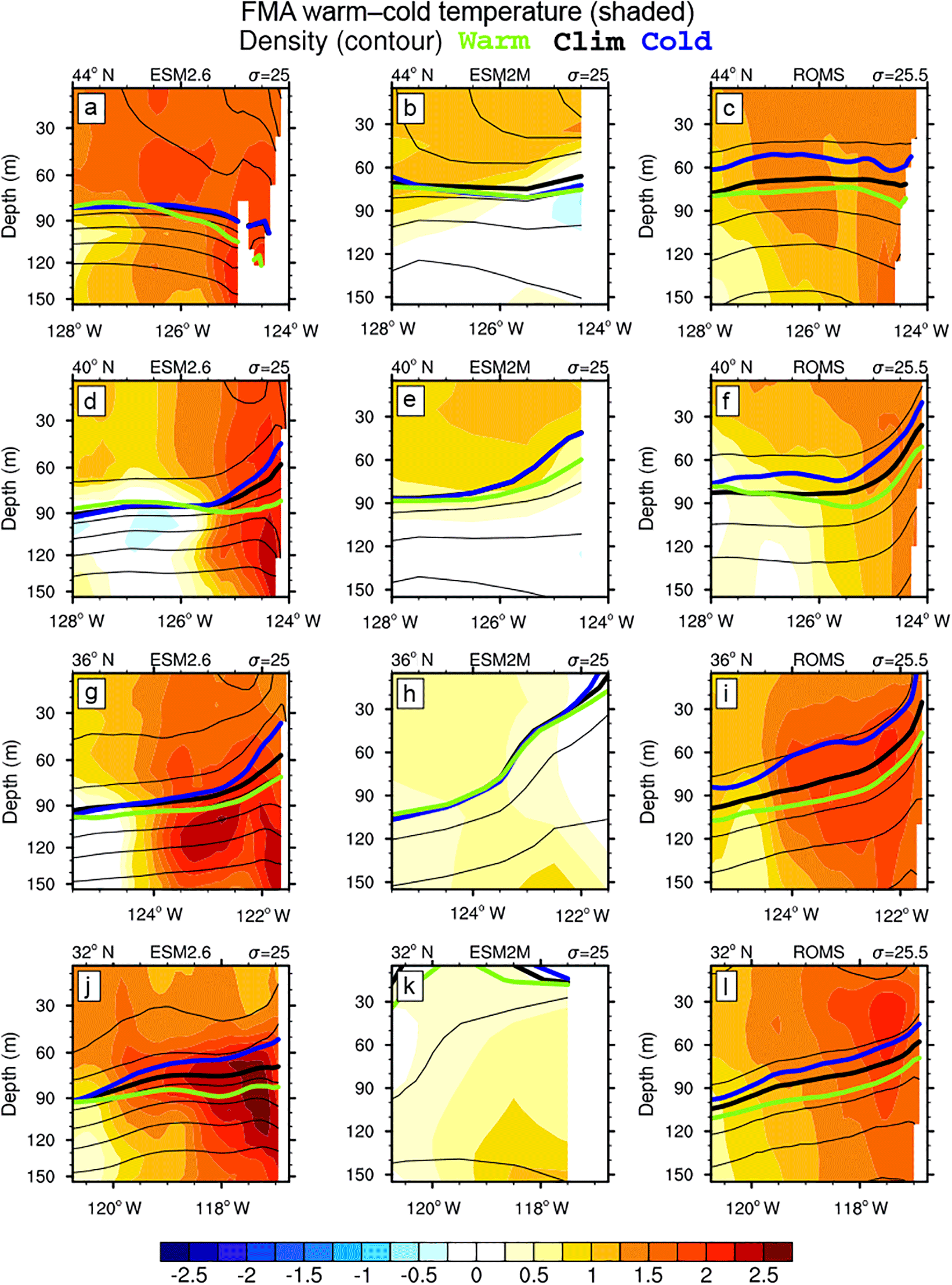
Figure 2ESM2.6 depth–longitude cross sections of FMA warm–cold high-pass-filtered standardized anomalies of temperature (unitless) for (first column) ESM2.6, (second column) ESM2M, and (third column) ROMS. The contours show the mean climatological density lines (first row) 44∘ N, (second row) 40∘ N, (third row) 36∘ N, and (fourth row) 32∘ N for the 222 km nearest the US west coast. The bold lines show the positions for the σ=25 level (ESM2.6 and ESM2M) and the σ=25.5 level (ROMS) for the climatology (black), El Niño conditions (green), and La Niña conditions (blue), and the thin lines indicate density increments of 0.25.
The notation of 0, 0∕1, and 1, as used in Fig. 5, indicates the years during which an ENSO event starts and ends. Typically, events start around June of one year (year 0) and end in spring to summer of the following year (year 1), with a peak during NDJ (0∕1). We employ this terminology as used by Rasmusson and Carpenter (1982).
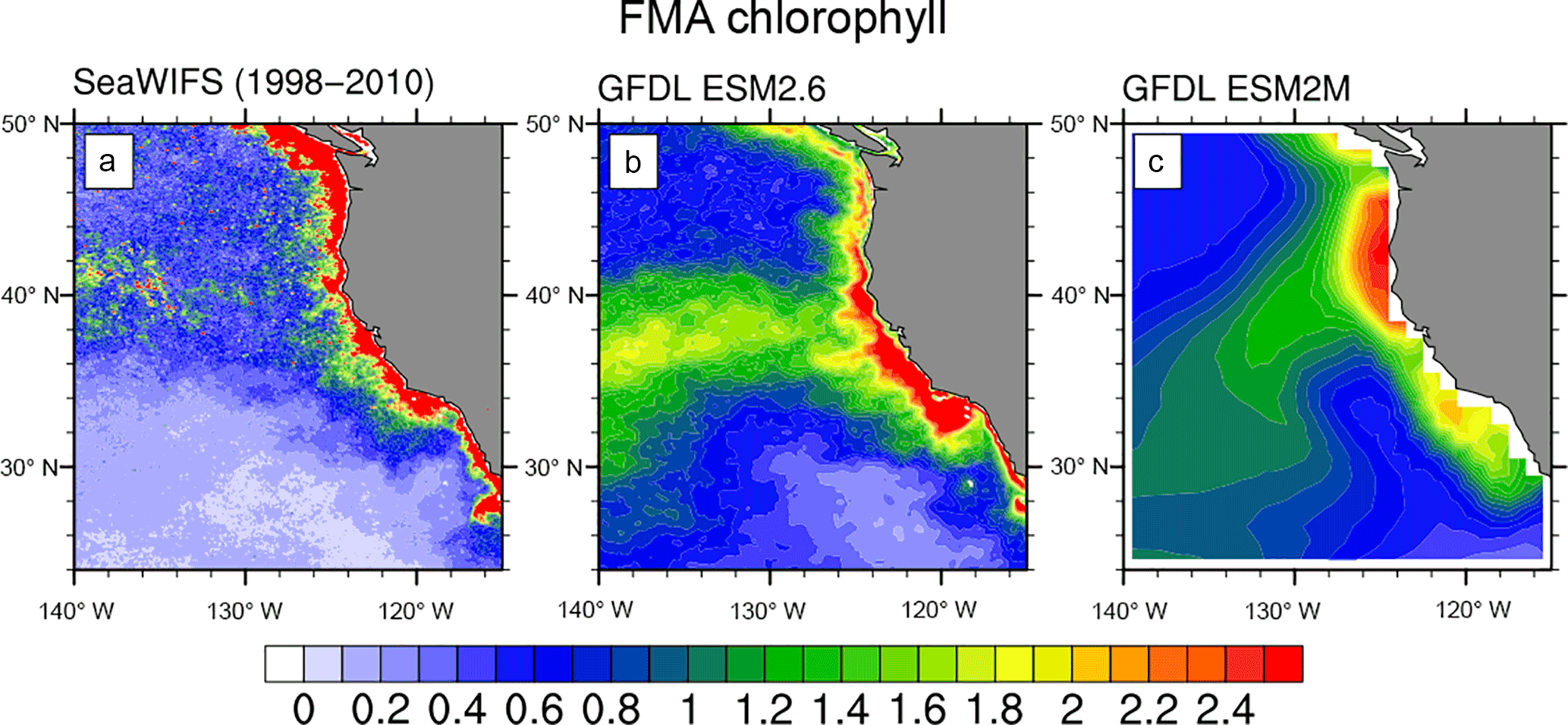
Figure 3FMA interannual standard deviation of surface chlorophyll concentrations (standardized by area average to produce comparable scales; unitless) for (a) 1998–2010 NASA SeaWiFS observations, (b) ESM2.6, and (c) ESM2M.
2.3 Comparison of modeled and observed ENSO in the North Pacific
To assess the model's performance in representing the physical regime of the North Pacific, we compare the physical manifestation of ENSO in ESM2.6 to a suite of observational data sets. In addition, we expand on this evaluation by comparing ESM2.6 to its GFDL precursor model, ESM2M, which has a horizontal oceanic resolution of 1∘. We use a 500-year pre-industrial ESM2M control run without transient atmospheric CO2 forcing. Since we analyze normalized values, differences in the magnitude of ENSO and its impact on the CalCS ecosystem would be taken into account between the two runs, including the possible influence of different atmospheric CO2 concentrations.
A comparison of climatological SST from the Hadley Centre Sea Ice and Sea Surface Temperature data set (HadISST) and sea level pressure (SLP) from NCEP reanalysis over the North Pacific reveals that both models simulate well the climatological mean SST signal and range as well as the position and magnitude of the North Pacific high pressure system off the southern US west coast and the Aleutian Low in the Gulf of Alaska (Fig. 1a, d, and g). During El Niño (La Niña), both models represent the composite average SST signals over the whole North Pacific with positive (negative) SST anomalies along the Equator and in the Gulf of Alaska and negative (positive) SST anomalies in the subtropical gyre around 30∘ N (Fig. 1b, c, e, f, h, and i). Both models also simulate the intensification (weakening) of the Aleutian Low during El Niño (La Niña), though the changes are overestimated and biases in orientation relative to the observed record are apparent. It should be noted that both the orientation and position of the Aleutian Low in the observations and in ESM2.6 are likely affected by the limited number of events present in both time series and could lead to a bias in the results (Deser et al., 2017).
To shed light on the vertical structure of temperature and density, we compare four vertical offshore cross sections from the ESM2.6 and ESM2M models to output from a Regional Ocean Modeling System (ROMS) reanalysis of the CalCS (Fig. 2). We chose to use the ROMS reanalysis as a comparison as it has a high spatiotemporal resolution and combines the strengths of individual data sources with those of an unconstrained (i.e., no data assimilation) ocean model to yield a product that is more useful than either of those alone. The offshore cross sections are located at 44, 40, 36, and 32∘ N for the 222 km closest to the US west coast. The 1980–2010 ROMS reanalysis covers the CalCS at 0.1∘ (∼ 10 km) resolution, assimilates available satellite (SST, SSH) and in situ (temperature, salinity) data (see Neveu et al. (2016) for details), and has been used extensively to describe CalCS physical dynamics, particularly in response to ENSO variability (Jacox et al., 2015a, b, 2016). ESM2.6 and the ROMS reanalysis show similar results for the composite difference between warm and cold ENSO events, indicating a significantly improved representation of the CalCS ENSO response in ESM2.6 relative to ESM2M. All three models agree on the sign of the temperature anomalies during El Niño (although ESM2M underestimates the magnitude of these anomalies), and ESM2.6 and ROMS highlight the largest temperature anomalies in the nearshore region and above 150 m water depth. All three models agree that density surfaces tend to deepen during El Niño (green lines) and shoal during La Niña (blue lines), with a difference in depth of up to 30 m between mean El Niño and La Niña conditions.
Additionally, we compare springtime (February–March–April; FMA) variability of modeled versus observed NASA-SeaWiFS surface chlorophyll (CHL) concentrations along the US west coast (Fig. 3). Due to its brevity, the CHL record does not lend itself well to an ENSO composite analysis, so we analyze CHL interannual variations via the standard deviation. We find that ESM2.6 represents well the strong cross-shore gradient in CHL variability all along the coast, with high variability of up to 2.5 standard deviations near the shore and lower variability offshore. ESM2M, on the other hand, only manages to reconstruct the same nearshore values in the region between 40 and 45∘ N, but underestimates the cross-shore gradient significantly to the north and south of this. Both models overestimate the CHL variability offshore at around 36–40∘ N in comparison to the observed variability.
Finally, we compare modeled versus observed Niño3.4 indices and find that the SST variability in the tropical Pacific is overestimated in both models, with the maximum SST variance in ESM2.6 being roughly twice as high as in ESM2M and up to 5 times higher than in the observations (see Fig. S2). Both models simulate the large-scale atmospheric and oceanic responses associated with ENSO. However, ENSO events that are similar in magnitude to the strongest on record are far more common and regular in the model than the recent historical record suggests. This offers an opportunity to isolate large ENSO signals, though even with normalization the biogeochemical imprint of ENSO events is likely accentuated relative to other sources of variation. Furthermore, due to its high horizontal oceanic resolution, ESM2.6 does a particularly good job of reproducing the cross-shore gradients in SST and CHL along the US west coast, with warm temperatures and increased CHL variability close to the coast. ESM2M's coarse horizontal resolution, on the other hand, does not allow for a representation of finer-scale processes related to coastal upwelling, and it thus fails to correctly model the cross-shore SST and CHL gradients. We thus focus on ESM2.6 to gain insight into the regional biogeochemical response of the CalCS to strong ENSO events.
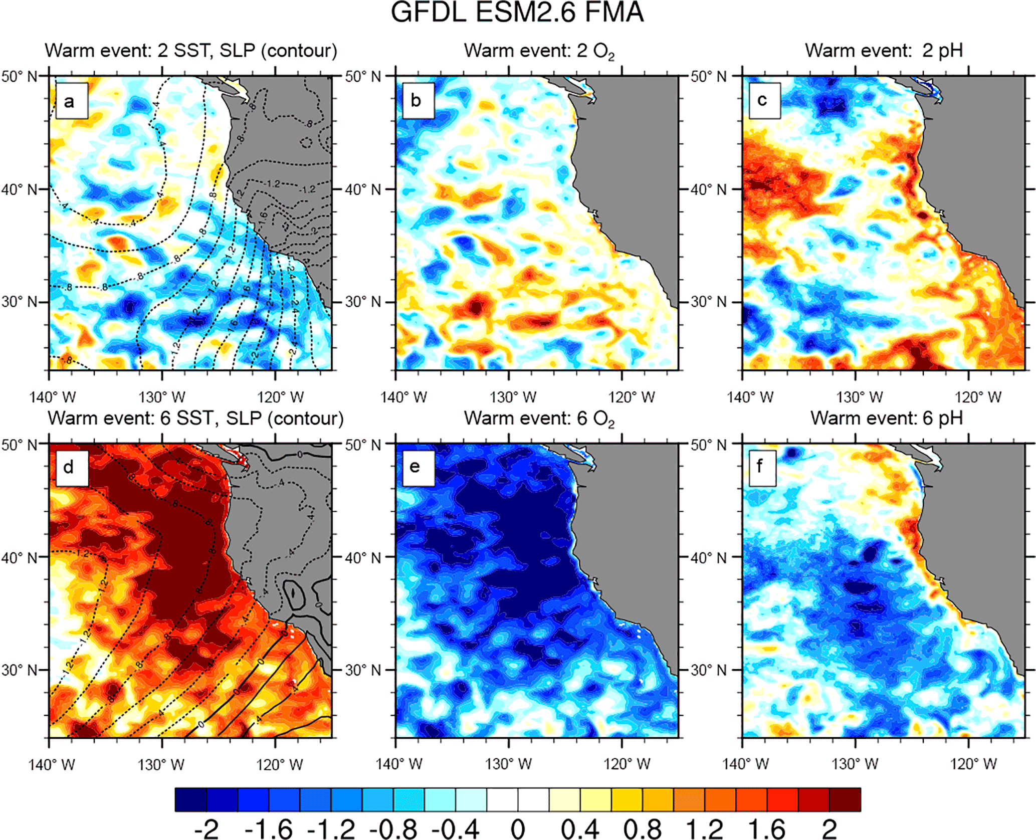
Figure 4ESM2.6 FMA high-pass-filtered standardized anomalies (unitless) for two warm El Niño events based on NDJ Niño3.4 anomalies: (a–c) event 2 and (d–f) event 6, with panels (a) and (d) displaying sea surface temperature with sea level pressure (0.2σ interval contours), (b) and (e) surface O2, and (c) and (f) surface pH.
3.1 Individual representations of ENSO in ESM2.6 in the CalCS
Figure 4 highlights the variability in SST (with overlaid SLP), O2, and pH between two of the six El Niño events (event 2 and event 6; see Figs. S3–S5 for the other four El Niño events and Fig. S5 for the individual SST/SLP La Niña events). The responses of all three variables to the different events are highly variable. While some of the SST/SLP responses are similar to the signals typical during an Eastern Pacific-type El Niño in the observational record (see the Supplement), the responses to event 2 and event 6 are drastically different from each other and from observed signals. For SST, O2, and pH, Fig. 4a–c show widespread areas of alternating negative and positive anomalies with no clear gradients between the coast and offshore. For event 6, on the other hand, all three variables exhibit stronger anomalies, covering broader areas offshore (Fig. 4d–f).
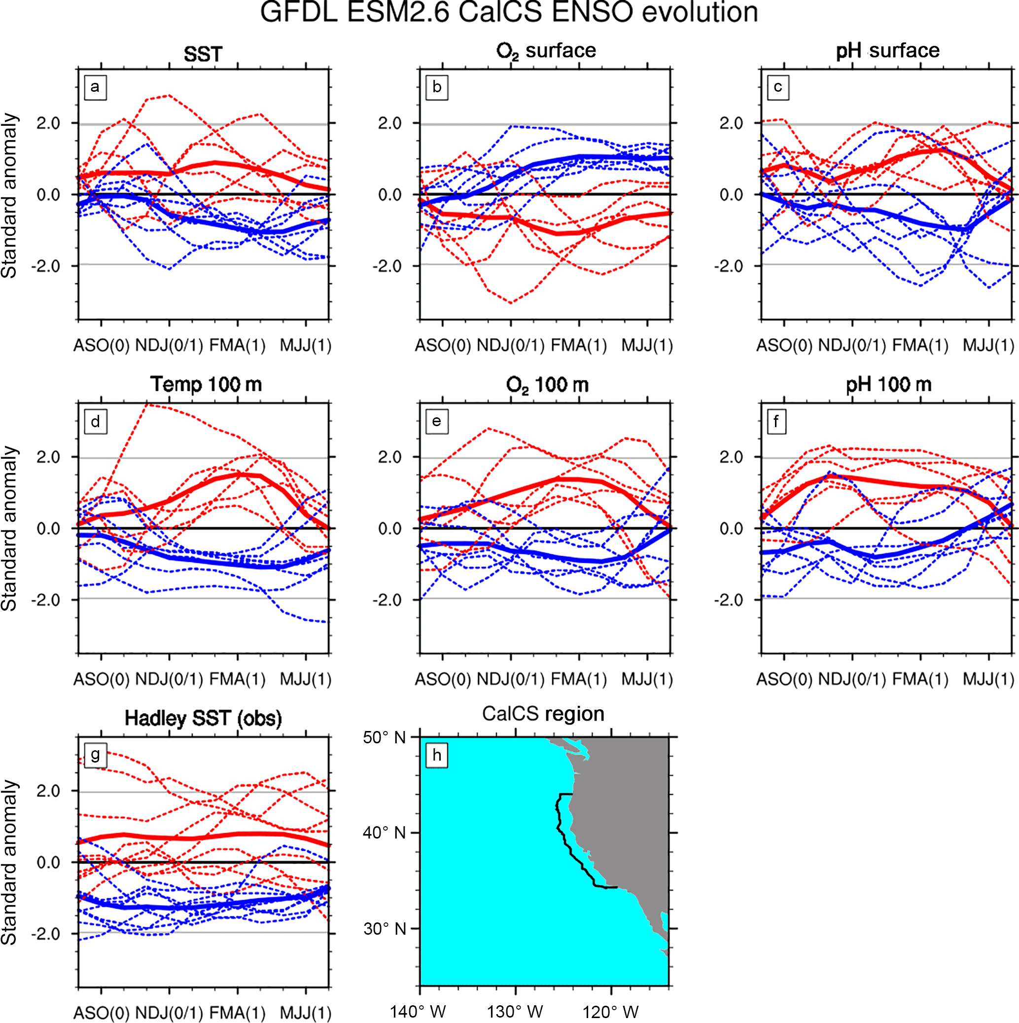
Figure 5Temporal evolution of individual warm (red) and cold (blue) events (dashed) and composite of all events (solid) for area averages between 34 and 44∘ N and 100 km offshore of the US west coast for (a) ESM2.6 sea surface temperature, (b) ESM2.6 surface O2, (c) ESM2.6 surface pH, (d) ESM2.6 100 m temperature, (e) ESM2.6 100 m O2, (f) ESM2.6 100 m pH, and (g) HadISST sea surface temperature. The time series are high-pass filtered and seasonally averaged and show the evolution of standardized anomalies (unitless) during the peak ENSO years from July–August–September (JAS) before the peak to June–July–August (JJA) after the peak. The black outline in panel (h) highlights the area within the CalCS used for this analysis. The notation of 0∕1 is as used in Rasmusson and Carpenter (1982).
Figure 5a–f show the temporal evolution of surface and subsurface (100 m) temperature, O2, and pH for the six individual El Niño and seven individual La Niña events, as well as the composite mean, for a region within 100 km of the coast and averaged over 34–44∘ N (see Fig. 5h for the specified region). We analyze the surface as well as 100 m since the surface is where heat transfer and chemical interactions with the atmosphere take place, and thus the atmospheric impact of ENSO is the greatest, and 100 m is roughly the depth of the heart of the thermocline. In addition to the modeled results, we show SST from the Hadley Center (HadISST; Fig. 5g). At the surface, temperature anomalies are on average positive (negative) during El Niño (La Niña) with values of −1σ to 3σ (−2σ to 1σ) for the individual events (Fig. 5a and d). On average, the variability of modeled SST (Fig. 5a) compares well with the observed SST (Fig. 5g), both for El Niño and La Niña, and especially for the composite mean. In the case of O2, the coastal surface waters experience lower-than-usual O2 conditions during El Niño (σ on average around −1), whereas O2 concentrations tend to be elevated with σ of up to 1 during La Niña (Fig. 5b). At 100 m, the strongest temperature signal occurs during the spring (FMA) following the typical El Niño season (NDJ). Furthermore, the CalCS experiences higher-than-usual O2 conditions during El Niño and lower O2 concentrations during La Niña at 100 m. As was the case with temperature, the largest O2 signal occurs with σ between 1 and 2 during FMA. This contrasting behavior exhibited by O2 at the surface and at 100 m is not exhibited by pH, which like temperature displays a consistent signal throughout the water column (Fig. 5c and f).
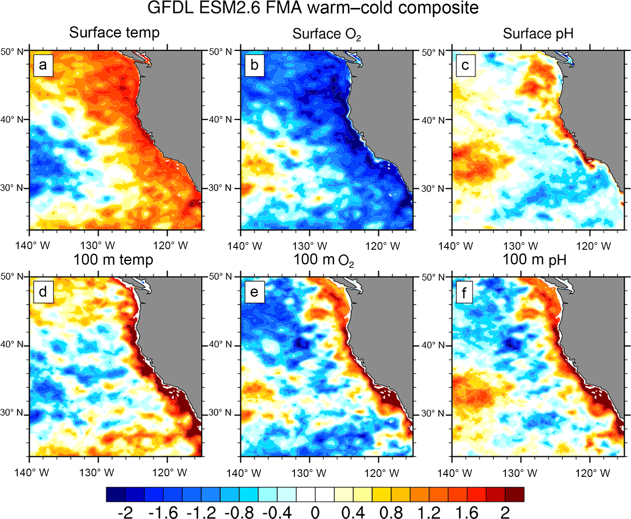
Figure 6ESM2.6 FMA warm–cold high-pass-filtered standardized anomalies (unitless) for (a) sea surface temperature, (b) surface O2, (c) surface pH, (d) 100 m temperature, (e) 100 m O2, and (f) 100 m pH.
As the results in Figs. 4 and 5 show, the variability between individual events is extremely high. Due to this fact, we focus our analyses on the composite mean over all El Niño and La Niña events for the remainder of the study.
3.2 Response of temperature, O2, and pH to mean ENSO signal
We illustrate the mean response of surface temperature, O2, and pH to ENSO in Fig. 6a–c. SST anomalies here are positive between the coast and ∼ 300–500 km offshore, as well as offshore north of 40∘ N and south of 28∘ N, with anomalies of up to 2σ (Fig. 6a). Offshore between ∼ 28 and 40∘ N, in the region of the subtropical gyre, SST anomalies are negative around 1–2σ and reflect a typical observed El Niño signal. The surface O2 anomalies largely reflect the SST signal, albeit with a reversed sign, as would be expected from a solubility-driven response. Close to the US west coast, O2 anomalies are lower than −2σ and become less negative further offshore. Positive O2 anomalies of around 0.8–2σ are found offshore in the region of the subtropical gyre (Fig. 6b). The surface pH signal differs from the SST and O2 signals, in that positive pH anomalies, with a maximum around 2σ, are limited to a very narrow band of ∼ 100 km along the coast (Fig. 6c). Between 100 km and around 500 km offshore, El Niño minus La Niña pH anomalies are negative around −0.8σ, while further offshore in the region of the subtropical gyre, pH anomalies are predominantly positive again.
We investigate ENSO-driven changes in temperature, O2, and pH in the subsurface (100 m) area in Fig. 6d–f. A similar cross-shore gradient in temperature occurs at 100 m compared to the surface, with anomalies larger than 2σ in some regions along the coast (Fig. 6d). However, the 100 m signal is more limited to within a ∼ 100 km wide band along the coast. The mean response of 100 m O2 to ENSO is drastically different than the O2 response at the surface, with positive anomalies within a 100 km band along the coast, indicating that two different processes govern the O2 response to ENSO at the surface and at depth (Fig. 6e). The 100 m pH signal looks largely the same as the surface pH signal, with a slightly broader cross-shore region with positive pH anomalies of up to 2σ (Fig. 6f). These positive pH anomalies are also more widespread northward and southward along the coast at 100 m compared to the surface. Furthermore, the 100 m pH signal is very similar to the 100 m O2 signal (compare Fig. 6e and f), suggesting a common subsurface process influencing both variables.
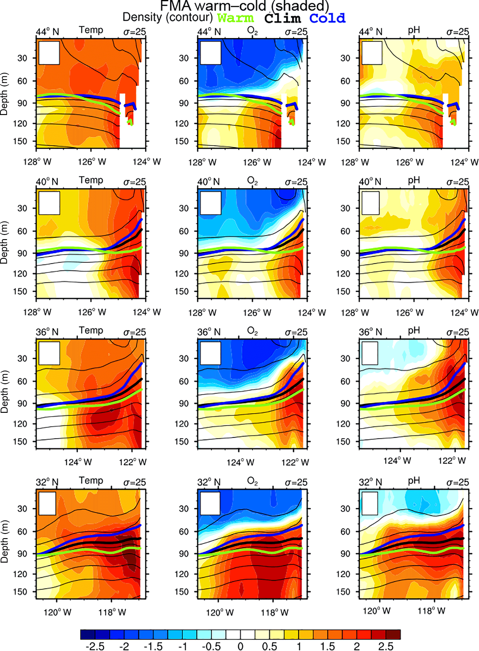
Figure 7ESM2.6 depth–longitude cross sections of FMA warm–cold high-pass-filtered standardized anomalies (unitless) of (first column) temperature, (second column) O2, and (third column) pH (shaded) with mean climatological density lines (contour) along (first row) 44∘ N, (second row) 40∘ N, (third row) 36∘ N, and (fourth row) 32∘ N for the 222 km nearest the US west coast. The bold lines show the positions for the σ=25 level for the climatology (black), El Niño conditions (green), and La Niña conditions (blue), and the thin lines indicate density increments of 0.25.
In Fig. 7, we examine the same offshore cross sections as in Fig. 2 and focus on the response of temperature, O2, and pH to ENSO in the vertical plane. Again, we show El Niño minus La Niña composite anomalies. The differing response of O2 to ENSO at the surface and at 100 m that we observed in Fig. 6 is also clearly visible in all four offshore cross sections in Fig. 7b, e, h, and k. The pH (Fig. 7c, f, i, l) and O2 responses are very similar between 32 and 36∘ N, suggesting that here they are both affected by the same processes. Between 40 and 45∘ N, on the other hand, El Niño minus La Niña pH anomalies are mostly positive throughout the water column, indicating that in this region there is a different process at play affecting pH in the top ∼ 100 m as opposed to O2 at the same latitude.
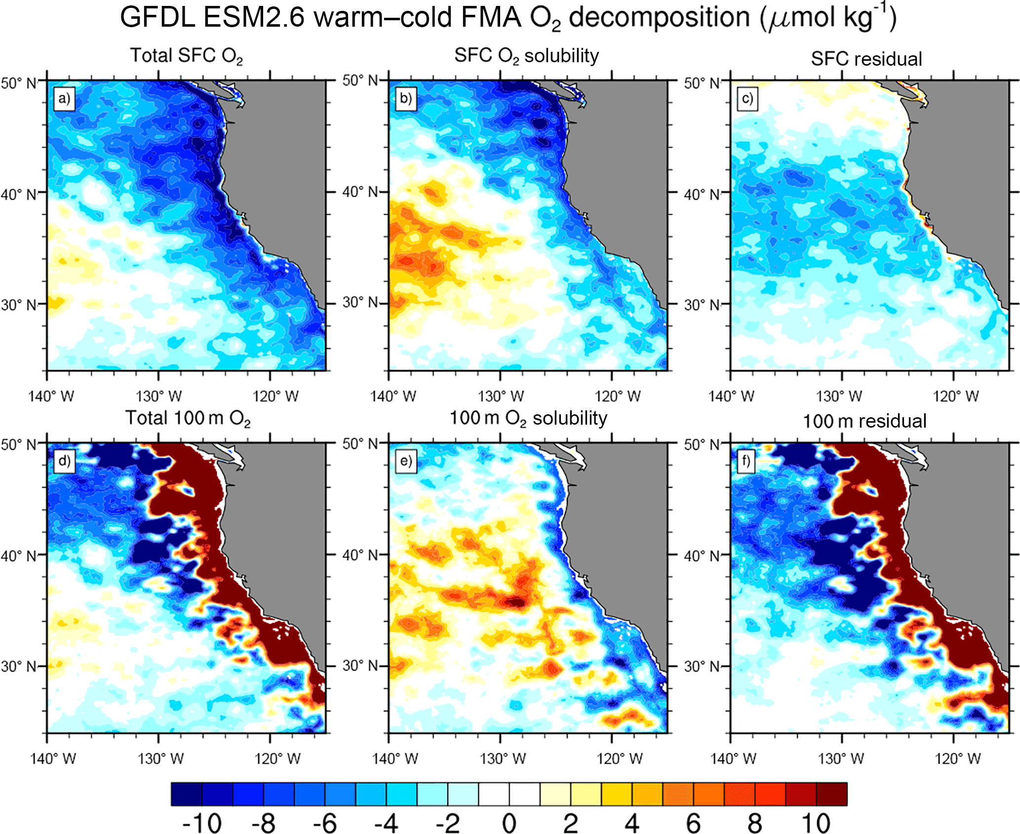
Figure 8ESM2.6 FMA warm–cold high-pass-filtered anomalies (µmol kg−1) for O2 and its components (a) surface total O2, (b) O2 due to Δ surface temperature (solubility), (c) residual surface processes, and (d) 100 m total O2, (b) O2 due to Δ 100 m temperature (solubility), (c) residual 100 m processes.
3.3 Drivers and processes behind changes in O2 and pH in the CalCS
In the surface ocean, O2 is affected by four main processes: (i) changes in SST, which affect the O2 solubility, (ii) wind-driven variability, which drives the O2 gas exchange across the air–sea interface, (iii) primary production, which reduces CO2 and increases O2 in the surface ocean, and (iv) ocean circulation, which affects horizontal advection and upwelling. We assume that the total change in O2 during El Niño is the sum of two components that include temperature-related and temperature-unrelated processes (after Fay and McKinley, 2013); thus,
For the analysis in Fig. 8, we derive the temperature-related component from the solubility of O2, using the solubility coefficients of Weiss (1970) as demonstrated in Sarmiento and Gruber (2006, p. 329). Since the total change in O2 is just the composite mean (ΔO2 in Eq. 1), we calculate the temperature-unrelated component, or residual term, from the difference between ΔO2 and the temperature-related component. The negative correlation between temperature and O2 in the surface ocean (as seen in Fig. 6a and b) can largely be explained by a rise in temperature causing a decrease in the amount of O2 that can be dissolved in the surface waters and thus leading to a drop in surface O2 (Fig. 8b). We argue that while increased storm activity during El Niño could enhance the O2 gas exchange through the air–sea interface, the decrease in wind stress over the CalCS, which is typically associated with El Niño, is expected to have an overall reducing effect on the O2 gas exchange. As the CalCS is on average a source of O2 to the atmosphere (Sarmiento and Gruber, 2006), this effect contributes to an increase in O2 and thus opposes the solubility effect. The residual effect (Fig. 8c), which is a combination of upwelling of waters with a certain O2 signal and the biological imprint on O2 concentrations, acts on average to decrease O2 in the surface ocean. This is likely due to primary production being limited during El Niño (e.g., Bograd and Lynn, 2001).
At 100 m, where El Niño leads to an increase in O2 along the coast and up to ∼ 200 km offshore, the main driver of the O2 change is the residual term, i.e., the contribution that is not directly linked to changes in temperature (Fig. 8f). This term could include local biological effects and/or circulation-driven changes between water masses with different histories of O2 supply and consumption. In this case, the simulated O2 increase is consistent with the deepening of isopycnal surfaces during El Niño (Fig. 2), replacing older, O2-poor waters associated with dense subsurface waters in the CalCS, with less dense, elevated O2 waters. Figure 9 demonstrates that during El Niño, the depth at which oxygen falls below the hypoxic threshold (where O2 is ≤ 60 µmol kg−1) deepens on average by 20 m in the first 100 km along the coast from a mean climatological depth of around 300 m, representing a 6–7 % change. This deepening of O2-depleted waters, where remineralization rates are high, can help explain the modeled increase in O2 seen along the coast in Fig. 7b, e, h, and k, and Fig. 8d.
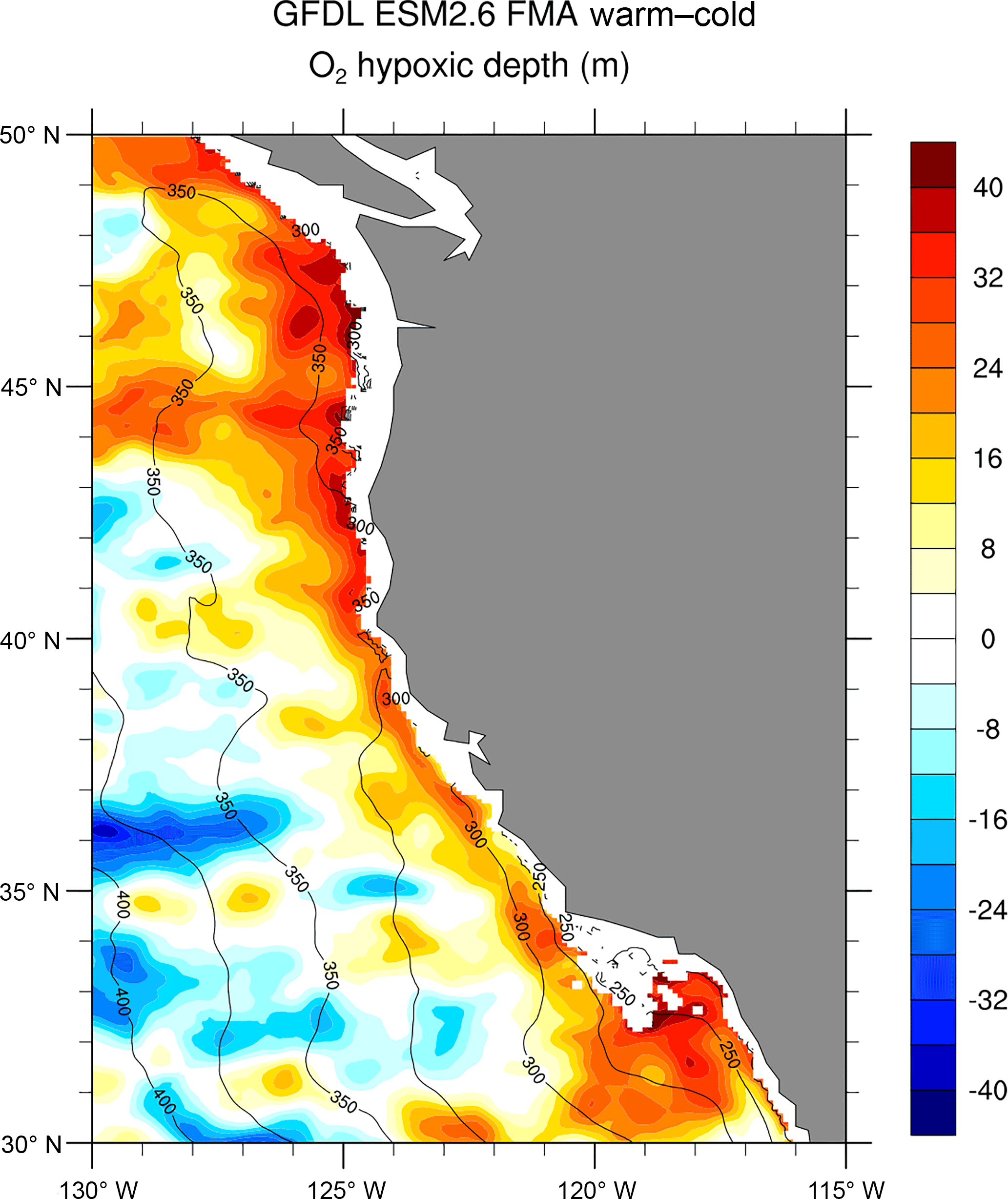
Figure 9ESM2.6 FMA warm–cold high-pass-filtered anomalies (m) for depth of the hypoxic threshold (O2 ≤ 60 µmol kg−1) and FMA mean climatological depth of the hypoxic threshold (25 m interval contours). White areas near the coast indicate an absence of the hypoxic level in the vertical layer. Positive numbers indicate a deepening of the hypoxic threshold.
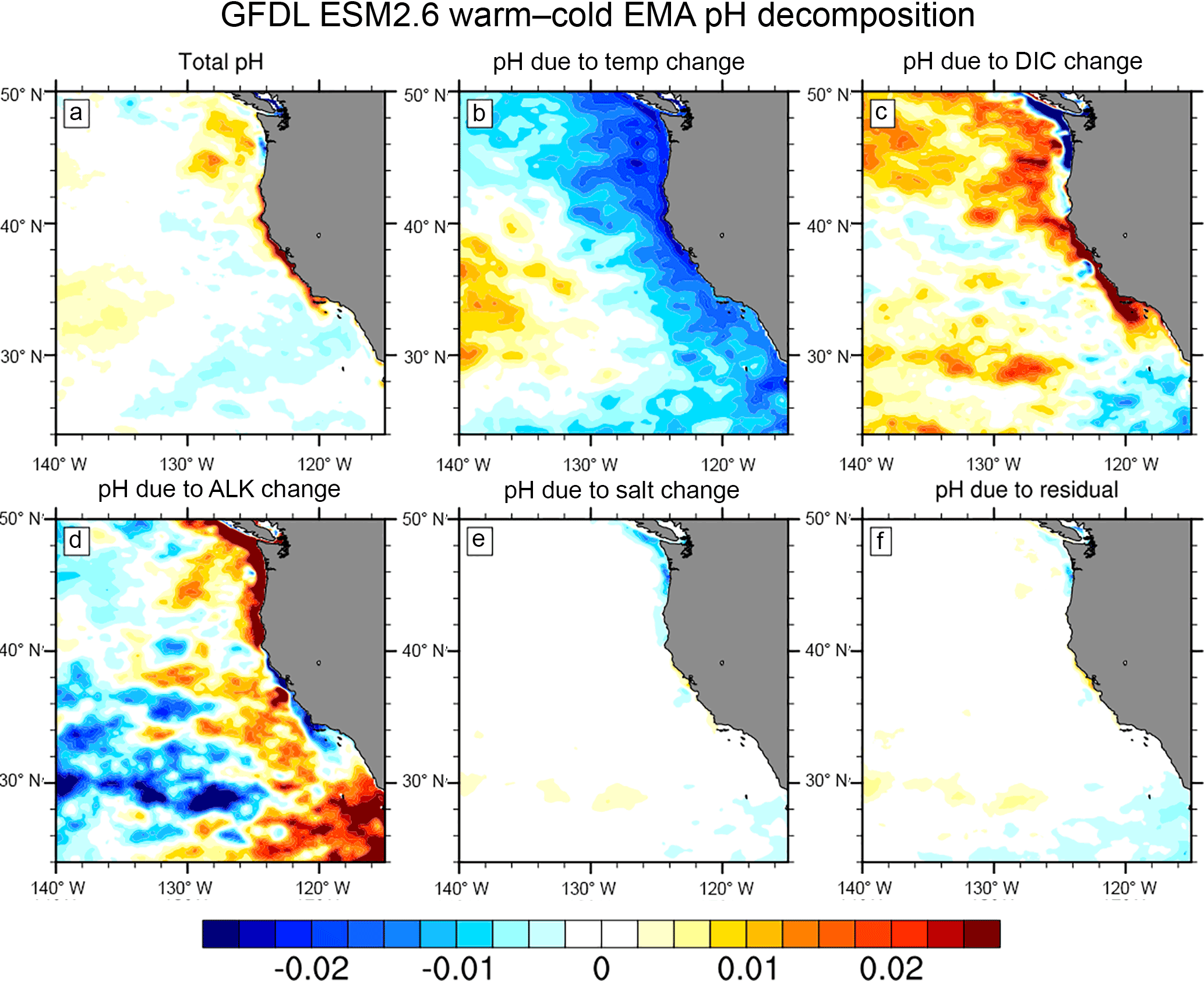
Figure 10ESM2.6 FMA warm–cold high-pass-filtered standardized anomalies for surface pH (unitless) and its components (a) total pH, (b) pH due to Δ temperature, (c) pH due to Δ dissolved inorganic carbon, (d) pH due to Δ total alkalinity, (e) pH due to Δ salinity, and (f) residual processes.
We consider the contributions of surface DIC, ALK, temperature (T), and salinity (S) to ENSO-driven changes in surface pH in Fig. 10. For this analysis, we focus on surface values, as DIC and ALK were saved only in the surface layer in the simulation. To decompose pH into these four drivers, we use a Taylor expansion according to the following equation (after Lovenduski et al., 2007; Doney et al., 2009b; Turi et al., 2014, 2016):
where the partial derivatives denote the sensitivities of pH to small changes in the four drivers. We determined these sensitivities by adding a small perturbation to each driver and recalculating pH with these new values using the online tool “CO2calc” (Robbins et al., 2010). We did this procedure for each driver and then multiplied each sensitivity by the change in each variable as calculated in the ENSO composites shown in Fig. 8 (corresponding to the Δ terms in Eq. 2).
Changes in DIC are primarily what drive the increase in pH in the nearshore 100 km region of the central CalCS (34–40∘ N; Fig. 10c), whereas the contributions from SST and ALK counteract the effect of DIC by reducing pH in the same region (Fig. 10b and d). During El Niño, upwelling is weakened and the thermocline is depressed, thus limiting the supply of low-pH and high-DIC waters to the surface. Likewise, the supply of cold, high-ALK waters is inhibited, leading to a decrease in pH due to a positive correlation with ALK and a negative correlation with temperature. North of ∼ 40∘ N, changes in DIC and SST contribute to an overall slight decrease in pH, whereas changes in ALK lead to an increase in pH. Thus, the SST contribution to pH mainly acts through the mechanism of surface heat fluxes, rather than through changes to the upwelling of cooler waters, as the contribution of changes in SST to the overall changes in pH (Fig. 10b) are of the same sign all along the coast and extend further offshore than the contributions of both DIC and ALK. The contributions of salinity and of the residual term are negligible throughout the whole CalCS (Fig. 10e and f).
The influence of ENSO on the physics and ultimately the biogeochemistry of the CalCS is very complex, due to the multiple processes that are affected by ENSO-driven climate variability. In this study, we delved into the processes through which ENSO can influence O2 and pH in the CalCS, and explained how physical variability can influence the carbon and oxygen systems of the CalCS. Our results demonstrate that in the surface ocean above the thermocline (above ∼ 100 m), interannual variability associated with ENSO modulates O2 and pH through two different mechanisms. In the case of surface O2, the strongest signal extends hundreds of kilometers offshore, mirroring the SST signal where elevated temperatures during El Niño lower the O2 solubility and thus cause a decrease in O2. The decomposition of O2 into temperature-related and temperature-unrelated components further confirmed that changes in the O2 solubility are the main driver for the surface O2 anomalies. Furthermore, our results show a decoupling between the response of O2 to ENSO in the surface ocean above the thermocline and the waters below that. Below 100 m, O2 is mainly modulated through changes in the vertical structure which affect the depth and location of the hypoxic threshold. During El Niño, for example, while the surface ocean above the thermocline experiences a decrease in O2, the concentration of O2 in the waters below that increases and the hypoxic threshold deepens due to a depression of the thermocline. During La Niña, the mechanism is reversed, and we model an increase in O2 at the surface and a decrease below 100 m (not shown). In the case of pH, on the other hand, the strongest changes occur in and are limited to a narrow band of ∼ 100 km along the central US west coast (∼ 34–40∘ N), both at the surface and below the thermocline. We inferred from the decomposition of pH into its individual components that changes in DIC, driven by modifications to the depth of the thermocline during an ENSO event, are the main driver of pH variability in the nearshore 100 km region, whereas temperature and ALK counteract the DIC effect. Further offshore, on the other hand, SST changes become more important in determining pH variability and the contributions of DIC and ALK tend to cancel each other. These results also suggest that during La Niña, the first 50–100 km along the coast are more readily supplied with cool, nutrient-rich water, thus enhancing the coastal upwelling effect, and potentially fueling biological production. At the same time, this process also brings more [H+], DIC, and ALK to the surface, thus overall lowering surface pH more toward a state of acidity. During El Niño, on the other hand, this process is suppressed, thus limiting the supply of nutrients and inhibiting biological production. At the same time, however, the supply of [H+] is also limited, therefore having an overall increasing effect on surface pH.
The findings for pH are in line with Nam et al. (2011), who noted an increase in nearshore surface pH during El Niño and a decrease during La Niña due to an uplifting of isopycnal surfaces and thus a higher supply of low-pH waters to the surface. In the case of O2, on the other hand, our results differ from what Nam et al. (2011) concluded. While we found a significant increase (decrease) in O2 in the nearshore surface waters above 100 m during La Niña (El Niño), their study suggests that during the 2010/2011 La Niña, O2 anomalies were lower than average. Their explanation for this observation is that due to an increased poleward flow of the California Undercurrent during La Niña, subsurface primary production was limited and thus caused a reduction in O2 concentrations. Our results however suggest that the modeled increase (decrease) in surface O2 during La Niña (El Niño) is mainly driven by changes to the O2 solubility due to anomalous surface cooling (warming). Furthermore, the analysis suggests that below 100 m, the opposing decrease (increase) in nearshore O2 during La Niña (El Niño) is attributable to a shoaling (deepening) of isopycnal surfaces, affecting the location of low-O2 waters. One potential between our study and the one by Nam et al. (2011) is that our study focuses on a composite mean ENSO signal over several events and the focus of theirs is on a specific event.
As Nam et al. (2011) pointed out, the large variability in O2 and pH during ENSO events seen in their study, which can be seen also in ours, suggests that the carbonate ion concentration ([CO]) and thus the saturation state of aragonite (Ωarag) experience similar fluctuations in their amplitude (Turi et al., 2016). If the pH drops below 7.75, which corresponds to Ωarag<1, waters become unfavorable for calcifying organisms to build and maintain their shell structure (e.g., Feely et al., 2008; Bednaršek et al., 2014; Bednaršek and Ohman, 2015). Our results suggest that during La Niña, the surface waters are more corrosive but also more oxygenated than during El Niño, while the waters below 100 m are both more corrosive and more deoxygenated. While primary production in the CalCS is greater during La Niña, the ecosystem is also more stressed by O2, low-pH, and low-Ωarag conditions which could add to or enhance the impact of these stressors due to climate change, as also noted by Nam et al. (2011). A more in-depth, quantitative analysis of the biological and physical mechanisms driving O2 and pH in the CalCS is anticipated to be the focus of future publications on ESM2.6.
This modeling study can help inform future observational studies on the frequency as well as horizontal and vertical resolution of O2 and pH measurements necessary to capture the surface and subsurface biogeochemical expressions of ENSO in the CalCS. We show that it is critical to have a strong observational network particularly in the nearshore 100 km region along the US west coast, as this is where the ENSO signal is largest, both in O2 and in pH. Furthermore, the modeled contrasting response of O2 to ENSO at the surface and at 100 m highlights the necessity of having vertical sections that go deep enough and have a sufficient vertical resolution to capture signals both in the euphotic zone above the thermocline as well as in the waters below it. This study additionally demonstrates that the diversity of ENSO events might contribute to the variability of the physics and biogeochemistry in the CalCS, and thus emphasizes the importance of analyzing long-enough time series to include a variety of different events. In addition to the variability between different types of ENSO events, other sources of internal climate variability unrelated to ENSO contribute to noisiness in the physical and biogeochemical signals in the CalCS (e.g., Deser et al., 2017).
While there is a clear link between ENSO events in the equatorial Pacific and ocean conditions in the CalCS, the evolution of any single event can be influenced by a number of processes. Each ENSO event evolves differently (e.g., Capotondi et al., 2015) and the variability between events, including the timing, strength, and location of temperature anomalies, can influence atmospheric teleconnections over the North Pacific (e.g., Calvo et al., 2017) and the propagation of coastally trapped waves (e.g., Frischknecht et al., 2015, 2017). Atmospheric teleconnections, and the associated winds and air temperatures over the CalCS, are influenced by SSTs in other basins, including the Indian Ocean (e.g., Annamalai et al., 2007; Han et al., 2013) and the Kuroshio–Oyashio extension in the western North Pacific (e.g., Smirnov et al., 2015) and potentially by Arctic sea-ice concentrations (e.g., Alexander et al., 2004; Screen et al., 2014). Differences in the state of the atmosphere and ocean at the time of an ENSO event also influence the magnitude of the anomalies and their evolution. Base state differences, such as changes in the position of the jet stream or decadal variability in the Pacific, can arise from variability on interannual to centennial timescales (e.g., Li et al., 2011; Zhou et al., 2014). The climate system is highly nonlinear and generates variability unrelated to ENSO events, contributing noisiness in the physical and biogeochemical ENSO-related signals in the CalCS. The noise is quite large, as has been demonstrated by the spread in ensembles of model simulations with the same ENSO conditions in the tropical Pacific but slightly different initial conditions (e.g., Hoerling and Kumar, 1997; Sardeshmukh et al., 2000; Alexander et al., 2002; Deser et al., 2017). Thus, the evolution of anomalies in the CalCS is expected to differ between ENSO events in both nature and models, which may partly explain the difference between the study by Nam et al. (2011), which analyzed a single La Niña event, and the present study. The uncertainty in the extratropical response to ENSO emphasizes the importance of analyzing long-enough time series to include a variety of different events.
The ROMS reanalysis output is available from http://oceanmodeling.ucsc.edu (Neveu et al., 2016). The GFDL model output is available upon request. The SLP observational data are from the NCEP reanalysis and were downloaded at https://www.esrl.noaa.gov/psd/data/gridded/ (Kalnay et al., 1996). The SST observational data are from the Hadley Centre at http://www.metoffice.gov.uk/hadobs/hadisst/ (Rayner et al., 2003). Finally, the CHL data are from SeaWiFS (1998–2010) and were obtained from NASA at https://doi.org/10.5067/ORBVIEW-2/SEAWIFS_OC.2014.0 (NASA, 2016).
The supplement related to this article is available online at: https://doi.org/10.5194/os-14-69-2018-supplement.
GT wrote the manuscript. GT, MA, CS, and JD outlined the initial stages of the project. GT, MA, NSL, AC, and JS were responsible for streamlining the direction and scope of the project. JS created all the figures. MJ supplied the ROMS simulation output. CS, JD, and JJ set up and ran the ESM2.6 and ESM2M models. JJ managed the model output and storage. All authors contributed to the discussion and revision of the manuscript contents.
The authors declare that they have no conflict of interest.
The authors thank Matthew Newman from NOAA/ESRL for his support and help in
outlining the initial stages of the project. All authors are grateful to the
support from NOAA's Climate Program Office through the Marine Tipping Points
program. NSL is grateful for support from NSF (OCE-1558225).
Edited by: Mario Hoppema
Reviewed by: three
anonymous referees
Alexander, M.: Extratropical Air-Sea Interaction, Sea Surface Temperature Variability, and the Pacific Decadal Oscillation, in: Clim. Dynam.: Why Does Climate Vary?, edited by: De-Zheng, S. and Bryan, F., 189, 123–148, AGU Geophysical Monograph Series, 2010. a
Alexander, M. A., Bladé, I., Newman, M., Lanzante, J. R., Lau, N. C., and Scott, J. D.: The atmospheric bridge: The influence of ENSO teleconnections on air-sea interaction over the global oceans, J. Climate, 15, 2205–2231, 2002. a, b, c
Alexander, M. A., Bhatt, U. S., Walsh, J. E., Timlin, M. S., Miller, J. S., and Scott, J. D.: The atmospheric response to realistic Arctic sea ice anomalies in an AGCM during winter, J. Climate, 17, 890–905, 2004. a
Annamalai, H., Okajima, H., and Watanabe, M.: Possible impact of the Indian Ocean SST on the Northern Hemisphere circulation during El Niño, J. Climate, 20, 3164–3189, 2007. a
Bakun, A.: Global climate change and intensification of coastal ocean upwelling, Science, 247, 198–201, 1990. a
Bakun, A., Black, B. A., Bograd, S. J., García-Reyes, M., Miller, A. J., Rykaczewski, R. R., and Sydeman, W. J.: Anticipated effects of climate change on coastal upwelling ecosystems, Current Climate Change Reports, 1, 85–93, 2015. a
Bednaršek, N. and Ohman, M. D.: Changes in pteropod distributions and shell dissolution across a frontal system in the California Current System, Mar. Ecol. Prog. Ser., 523, 93–103, 2015. a, b
Bednaršek, N., Feely, R. A., Reum, J. C. P., Peterson, B., Menkel, J., Alin, S. R., and Hales, B.: Limacina helicina shell dissolution as an indicator of declining habitat suitability owing to ocean acidification in the California Current Ecosystem, P. R. Soc. B, 281, 20140123, https://doi.org/10.1098/rspb.2014.0123, 2014. a, b
Benson, S. R., Croll, D. A., Marinovic, B. B., Chavez, F. P., and Harvey, J. T.: Changes in the cetacean assemblage of a coastal upwelling ecosystem during El Niño 1997–98 and La Niña 1999, Prog. Oceanogr., 54, 279–291, 2002. a
Bograd, S. J. and Lynn, R. J.: Physical-biological coupling in the California Current during the 1997-99 E1 Niño-La Niña cycle, Geophys. Res. Lett., 28, 275–278, 2001. a, b
Bograd, S. J., Castro, C. G., Di Lorenzo, E., Palacios, D. M., Bailey, H., Gilly, W., and Chavez, F. P.: Oxygen declines and the shoaling of the hypoxic boundary in the California Current, Geophys. Res. Lett., 35, L12607, https://doi.org/10.1029/2008GL034185, 2008. a, b, c
Bopp, L., Resplandy, L., Orr, J. C., Doney, S. C., Dunne, J. P., Gehlen, M., Halloran, P., Heinze, C., Ilyina, T., Séférian, R., Tjiputra, J., and Vichi, M.: Multiple stressors of ocean ecosystems in the 21st century: projections with CMIP5 models, Biogeosciences, 10, 6225–6245, https://doi.org/10.5194/bg-10-6225-2013, 2013. a
Breitburg, D. L., Salisbury, J., Bernhard, J. M., Cai, W.-J., Dupont, S., Doney, S. C., Levin, L. A., Long, W. C., Milke, L. M., Miller, S. H., Phelan, B., Passow, U., Seibel, B. A., Todgham, A. E., and Tarrant, A. M.: And on top of all that… Coping with ocean acidification in the midst of many stressors, Oceanography, 28, 48–61, 2015. a
Calvo, N., Iza, M., Hurwitz, M. M., Manzini, E., Peña Ortiz, C., Butler, A. H., Cagnazzo, C., Ineson, S., and Garfinkel, C. I.: Northern Hemisphere Stratospheric Pathway of Different El Niño Flavors in Stratosphere-Resolving CMIP5 Models, J. Climate, 30, 4351–4371, 2017. a
Capotondi, A., Wittenberg, A. T., Newman, M., Di Lorenzo, E., Yu, J.-Y., Braconnot, P., Cole, J., Dewitte, B., Giese, B., Guilyardi, E., Jin, F.-F., Karnauskas, K., Kirtman, B., Lee, T., Schneider, N., Xue, Y., and Yeh, S.-W.: Understanding ENSO diversity, B. Am. Meteorol. Soc., 96, 921–938, 2015. a, b
Castro, C. G., Collins, C. A., Walz, P., Pennington, J. T., Michisaki, R. P., Friederich, G., and Chavez, F. P.: Nutrient variability during El Niño 1997–98 in the California current system off central California, Prog. Oceanogr., 54, 171–184, 2002. a
Chavez, F. P. and Messié, M.: A comparison of Eastern Boundary Upwelling Ecosystems, Prog. Oceanogr., 83, 80–96, 2009. a
Chavez, F. P., Collins, C. A., Huyer, A., and Mackas, D. L.: El Niño along the west coast of North America, Prog. Oceanogr., 54, 1–5, 2002. a
Checkley Jr., D. M. and Barth, J. A.: Patterns and processes in the California Current System, Prog. Oceanogr., 83, 49–64, 2009. a
Chelton, D. B., DeSzoeke, R. A., Schlax, M. G., El Naggar, K., and Siwertz, N.: Geographical Variability of the First Baroclinic Rossby Radius of Deformation, J. Phys. Oceanogr., 28, 433–460, 1998. a
Collins, C. A., Castro, C. G., Asanuma, H., Rago, T. A., Han, S. K., Durazo, R., and Chavez, F. P.: Changes in the hydrography of Central California waters associated with the 1997–98 El Niño, Prog. Oceanogr., 54, 129–147, 2002. a
Delworth, T. L., Rosati, A., Anderson, W., Adcroft, A. J., Balaji, V., Benson, R., Dixon, K., Griffies, S. M., Lee, H. C., Pacanowski, R. C., Vecchi, G. A., Wittenberg, A. T., Zeng, F., and Zhang, R.: Simulated climate and climate change in the GFDL CM2.5 high-resolution coupled climate model, J. Climate, 25, 2755–2781, 2012. a
Deser, C., Simpson, I. R., McKinnon, K. A., and Phillips, A. S.: The Northern Hemisphere extra-tropical atmospheric circulation response to ENSO: How well do we know it and how do we evaluate models accordingly?, J. Climate, 30, 5059–5082, 2017. a, b, c
DeWeaver, E. and Nigam, S.: Linearity in ENSO's Atmospheric Response, J. Climate, 15, 2446–2461, 2002. a
Diaz, R. J. and Rosenberg, R.: Spreading dead zones and consequences for marine ecosystems, Science, 321, 926–929, 2008. a
Di Lorenzo, E., Schneider, N., Cobb, K. M., Franks, P. J. S., Chhak, K., Miller, A. J., McWilliams, J. C., Bograd, S. J., Arango, H., Curchitser, E., Powell, T., and Rivière, P.: North Pacific Gyre Oscillation links ocean climate and ecosystem change, Geophys. Res. Lett., 35, L08607, https://doi.org/10.1029/2007GL032838, 2008. a
Di Lorenzo, E., Cobb, K. M., Furtado, J. C., Schneider, N., Anderson, B. T., Bracco, A., Alexander, M. A., and Vimont, D. J.: Central Pacific El Niño and decadal climate change in the North Pacific Ocean, Nat. Geosci., 3, 762–765, 2010. a
Dommenget, D., Bayr, T., and Frauen, C.: Analysis of the non-linearity in the pattern and time evolution of El Niño southern oscillation, Clim. Dynam., 40, 2825–2847, 2013. a
Doney, S. C.: The Growing Human Footprint on Coastal and Open-Ocean Biogeochemistry, Science, 328, 1512–1516, 2010. a
Doney, S. C., Fabry, V. J., Feely, R. A., and Kleypas, J. A.: Ocean Acidification: The Other CO2 Problem, Annu. Rev. Mar. Sci., 1, 169–192, 2009a. a
Doney, S. C., Lima, I., Feely, R. A., Glover, D. M., Lindsay, K., Mahowald, N., Moore, J. K., and Wanninkhof, R.: Mechanisms governing interannual variability in upper-ocean inorganic carbon system and air-sea CO2 fluxes: Physical climate and atmospheric dust, Deep-Sea Res. Pt. II, 56, 640–655, 2009b. a
Duchon, M. E.: Lanczos filtering in one and two dimensions, J. Appl. Meteorol., 18, 1016–1022, 1979. a
Dunne, J. P., Stock, C. A., and John, J. G.: Representation of Eastern Boundary Currents in GFDL's Earth System Models, California Cooperative Oceanic Fisheries Investigations Reports, 56, 72–75, 2015. a
Fay, A. R. and McKinley, G. A.: Global trends in surface ocean pCO2 from in situ data, Global Biogeochem. Cy., 27, 541–557, 2013. a
Feely, R. A., Sabine, C. L., Hernandez-Ayon, J. M., Ianson, D., and Hales, B.: Evidence for upwelling of corrosive “acidified” water onto the continental shelf, Science, 320, 1490–1492, 2008. a, b, c
Fiechter, J., Curchitser, E. N., Edwards, C. A., Chai, F., Goebel, N. L., and Chavez, F. P.: Air-sea CO2 fluxes in the California Current: Impacts of model resolution and coastal topography, Global Biogeochem. Cy., 28, 371–385, 2014. a
Franks, P. J. S., Di Lorenzo, E., Goebel, N. L., Chenillat, F., Rivière, P., Edwards, C. A., and Miller, A. J.: Modeling Physical-Biological Responses to Climate Change in the California Current System, Oceanography, 26, 26–33, 2013. a
Frischknecht, M., Münnich, M., and Gruber, N.: Remote versus Local Influence of ENSO on the California Current System, J. Geophys. Res.-Ocean, 120, 1353–1374, 2015. a, b
Frischknecht, M., Münnich, M., and Gruber, N.: Local atmospheric forcing driving an unexpected California Current System response during the 2015–2016 El Niño, Geophys. Res. Lett., 44, 304–311, 2017. a, b
Garcia, H. E., Locarnini, R. A., Boyer, T. P., and Antonov, J. I.: World Ocean Atlas 2005, Volume 3: Dissolved Oxygen, Apparent Oxygen Utilization, and Oxygen Saturation, in: NOAA Atlas NESDIS 63, edited by: Levitus, S., p. 342, U.S. Government Printing Office, Washington, DC, 2006a. a
Garcia, H. E., Locarnini, R. A., Boyer, T. P., and Antonov, J. I.: World Ocean Atlas 2005, Volume 4: Nutrients (phosphate, nitrate, silicate), in: NOAA Atlas NESDIS 64, edited by: Levitus, S., p. 396, U.S. Government Printing Office, Washington, DC, 2006b. a
Gray, J. S., Wu, R. S., and Or, Y. Y.: Effects of hypoxia and organic enrichment on the coastal marine environment, Mar. Ecol. Prog. Ser., 238, 249–279, 2002. a
Griffies, S. M.: Elements of the Modular Ocean Model (MOM): 2012 release, GFDL Ocean Group Technical Report No. 7, 3, 1–631, 2012. a
Griffies, S. M., Winton, M., Anderson, W. G., Benson, R., Delworth, T. L., Dufour, C. O., Dunne, J. P., Goddard, P., Morrison, A. K., Rosati, A., Wittenberg, A. T., Yin, J., and Zhang, R.: Impacts on ocean heat from transient mesoscale eddies in a hierarchy of climate models, J. Climate, 28, 952–977, 2015. a
Gruber, N.: Warming up, turning sour, losing breath: ocean biogeochemistry under global change, Philos. T. Roy. Soc. A, 369, 1980–1996, 2011. a
Han, W., Meehl, G. A., Hu, A., Alexander, M., Yamagata, T., Yuan, D., Ishii, M., Pegion, P., Zheng, J., Hamlington, B., Quan, X.-W., and Leben, R.: Intensification of decadal and multi-decadal sea level variability in the western tropical Pacific during recent decades, J. Climate, 43, 1357–1379, 2013. a
Hoerling, M. P. and Kumar, A.: Why do North American climate anomalies differ from one El Niño event to another?, Geophys. Res. Lett., 24, 1059–1062, 1997. a
Hoerling, M. P., Kumar, A., and Zhong, M.: El Niño, La Niña, and the nonlinearity of their teleconnections, J. Climate, 10, 1769–1786, 1997. a
Hopcroft, R. R., Clarke, C., and Chavez, F. P.: Copepod communities in Monterey Bay during the 1997–1999 El Niño and La Niña, Prog. Oceanogr., 54, 251–264, 2002. a
Huyer, A. and Smith, R. L.: The Signature of El Niño off Oregon, 1982–1983, J. Geophys. Res., 90, 7133–7142, 1985. a
Jacox, M. G., Moore, A. M., Edwards, C. A., and Fiechter, J.: Spatially resolved upwelling in the California Current System, Geophys. Res. Lett., 41, 3189–3196, 2014. a
Jacox, M. G., Bograd, S. J., Hazen, E. L., and Fiechter, J.: Sensitivity of the California Current nutrient supply to wind, heat, and remote ocean forcing, Geophys. Res. Lett., 42, 5950–5957, 2015a. a, b
Jacox, M. G., Fiechter, J., Moore, A. M., and Edwards, C. A.: ENSO and the California Current coastal upwelling response, J. Geophys. Res.-Ocean, 120, 1691–1702, 2015b. a, b, c, d
Jacox, M. G., Hazen, E. L., Zaba, K. D., Rudnick, D. L., Edwards, C. A., Moore, A. M., and Bograd, S. J.: Impacts of the 2015–2016 El Niño on the California Current System: Early assessment and comparison to past events, Geophys. Res. Lett., 43, 7072–7080, 2016. a
Kahru, M. and Mitchell, B. G.: Influence of the 1997–98 El Niño on the surface chlorophyll in the California Current, Geophys. Res. Lett., 27, 2937–2940, 2000. a
Kahru, M. and Mitchell, B. G.: Influence of the El Niño-La Niña cycle on satellite-derived primary production in the California Current, Geophys. Res. Lett., 29, 1846, https://doi.org/10.1029/2002GL014963, 2002. a
Kalnay, E., Kanamitsu, M., Kistler, R., Collins, W., Deaven, D., Gandin, L., Iredell, M., Saha, S., White, G., Woollen, J., Zhu, Y., Leetmaa, A., Reynolds, R., Chelliah, M., Ebisuzaki, W., Higgins, W., Janowiak, J., Mo, K. C., Ropelewski, C., Wang, J., Jenne, R., and Joseph, D.: The NCEP/NCAR 40-year reanalysis project, B. Am. Meteorol. Soc., 77, 437–471, https://doi.org/10.1175/1520-0477(1996)077<0437:TNYRP>2.0.CO;2, 1996 (data available at: https://www.esrl.noaa.gov/psd/data/gridded/, last access: 1 June 2016).
Key, R. M., Kozyr, A., Sabine, C. L., Lee, K., Wanninkhof, R., Bullister, J. L., Feely, R. A., Millero, F. J., Mordy, C., and Peng, T.-H.: A global ocean carbon climatology: Results from Global Data Analysis Project (GLODAP), Global Biogeochem. Cy., 18, GB4031, https://doi.org/10.1029/2004GB002247, 2004. a
Kosro, P. M.: A poleward jet and an equatorward undercurrent observed off Oregon and northern California, during the 1997–98 El Niño, Prog. Oceanogr., 54, 343–360, 2002. a
Kudela, R. M. and Chavez, F. P.: Multi-platform remote sensing of new production in central California during the 1997–1998 El Niño, Prog. Oceanogr., 54, 233–249, 2002. a
Lewis, E. and Wallace, D.: Program Developed for CO2 System Calculations, Tech. rep., ORNL/CDIAC-105. Carbon Dioxide Information Analysis Center, Oak Ridge National Laboratory, U.S. Department of Energy, Oak Ridge, Tennessee, 1998. a
Li, J., Xie, S.-P., Cook, E. R., Huang, G., D'Arrigo, R., Liu, F., Ma, J., and Zheng, X.-T.: Interdecadal modulation of El Niño amplitude during the past millennium, Nat. Clim. Change, 1, 114–118, 2011. a
Lovenduski, N. S., Gruber, N., Doney, S. C., and Lima, I. D.: Enhanced CO2 outgassing in the Southern Ocean from a positive phase of the Southern Annular Mode, Global Biogeochem. Cy., 21, GB2026, https://doi.org/10.1029/2006GB002900, 007. a
Lynn, R. J. and Bograd, S. J.: Dynamic evolution of the 1997–1999 El Niño-La Niña cycle in the southern California Current System, Prog. Oceanogr., 54, 59–75, 2002. a
Macias, D., Landry, M. R., Gershunov, A., Miller, A. J., and Franks, P. J. S.: Climatic control of upwelling variability along the western North-American coast, PloS one, 7, e30436, https://doi.org/10.1371/journal.pone.0030436, 2012. a
Mantua, N. J. and Hare, S. R.: The Pacific Decadal Oscillation, J. Oceanogr., 58, 35–44, 2002. a
Messié, M., Ledesma, J., Kolber, D. D., Michisaki, R. P., Foley, D. G., and Chavez, F. P.: Potential new production estimates in four eastern boundary upwelling ecosystems, Prog. Oceanogr., 83, 151–158, 2009. a
Murphree, T., Bograd, S. J., Schwing, F. B., and Ford, B.: Large scale atmosphere-ocean anomalies in the northeast Pacific during 2002, Geophys. Res. Lett., 30, 8026, https://doi.org/10.1029/2003GL017303, 2003. a
Nam, S., Kim, H.-J., and Send, U.: Amplification of hypoxic and acidic events by La Niña conditions on the continental shelf off California, Geophys. Res. Lett., 38, L22602, https://doi.org/10.1029/2011GL049549, 2011. a, b, c, d, e, f, g, h, i, j, k
Narayan, N., Paul, A., Mulitza, S., and Schulz, M.: Trends in coastal upwelling intensity during the late 20th century, Ocean Sci., 6, 815–823, https://doi.org/10.5194/os-6-815-2010, 2010. a
NASA: Goddard Space Flight Center, Ocean Ecology Laboratory, Ocean Biology Processing Group, Sea-viewing Wide Field-of-view Sensor (SeaWiFS) Ocean Color Data, 2014 Reprocessing, NASA OB.DAAC, Greenbelt, MD, USA, https://doi.org/10.5067/ORBVIEW-2/SEAWIFS_OC.2014.0, last access: 21 June 2016.
Neveu, E., Moore, A. M., Edwards, C. A., Fiechter, J., Drake, P., Crawford, W. J., Jacox, M. G., and Nuss, E.: An historical analysis of the California Current circulation using ROMS 4D-Var: System configuration and diagnostics, Ocean Model., 99, 133–151, https://doi.org/10.1016/j.ocemod.2015.11.012, 2016 (data available at: http://oceanmodeling.ucsc.edu, last access: 1 March 2017). a
Newman, M., Alexander, M. A., Ault, T. R., Cobb, K. M., Deser, C., Di Lorenzo, E., Mantua, N. J., Miller, A. J., Minobe, S., Nakamura, H., Schneider, N., Vimont, D. J., Phillips, A. S., Scott, J. D., and Smith, C. A.: The Pacific Decadal Oscillation, revisited, J. Climate, 29, 4399–4427, 2016. a
Pearcy, W. G.: Marine nekton off Oregon and the 1997–98 El Niño, Prog. Oceanogr., 54, 399–403, 2002. a
Peterson, W. T., Keister, J. E., and Feinberg, L. R.: The effects of the 1997–99 El Niño/La Niña events on hydrography and zooplankton off the central Oregon coast, Prog. Oceanogr., 54, 381–398, 2002. a
Rasmusson, E. M. and Carpenter, T. H.: Variations in Tropical Sea Surface Temperature and Wind Associated with the Southern Oscillation/El Niño, Mon. Weather Rev., 110, 354–384, 1982. a, b
Rayner, N. A., Parker, D. E., Horton, E. B., Folland, C. K., Alexander, L. V., Rowell, D. P., Kent, E. C., and Kaplan, A.: Global analyses of sea surface temperature, sea ice, and night marine air temperature since the late nineteenth century, J. Geophys. Res., 108, 4407, https://doi.org/10.1029/2002JD002670, 2003 (data available at: http://www.metoffice.gov.uk/hadobs/hadisst/, last access: 1 July 2016).
Robbins, L. L., Hansen, M. E., Kleypas, J. A., and Meylan, S. C.: CO2calc – A user-friendly seawater carbon calculator for Windows, Mac OS X, and iOS (iPhone), Tech. rep., U.S. Geological Survey Open-File Report 2010–1280, 2010. a
Ryan, H. F. and Noble, M.: Sea level response to ENSO along the central California coast: How the 1997–1998 event compares with the historic record, Prog. Oceanogr., 54, 149–169, 2002. a
Rykaczewski, R. R., Dunne, J. P., Sydeman, W. J., García-Reyes, M., Black, B. A., and Bograd, S. J.: Poleward displacement of coastal upwelling-favorable winds in the ocean's eastern boundary currents through the 21st century, Geophys. Res. Lett., 42, 6424–6431, 2015. a
Saba, V. S., Griffies, S. M., Anderson, W. G., Winton, M., Alexander, M. A., Delworth, T. L., Hare, J. A., Harrison, M. J., Rosati, A., Vecchi, G. A., and Zhang, R.: Enhanced warming of the Northwest Atlantic Ocean under climate change, J. Geophys. Res.-Ocean, 121, 118–132, 2016. a, b
Sardeshmukh, P. D., Compo, G. P., and Penland, C.: Changes of probability associated with El Niño, J. Climate, 13, 4268–4286, 2000. a
Sarmiento, J. L. and Gruber, N.: Ocean Biogeochemical Dynamics, Princeton University Press, Princeton, New Jersey, USA, 2006. a, b
Schwing, F. B., Gaxiola-Castro, G., Goméz-Valdéz, J., Kosro, P. M., Mantyla, A. W., Smith, R. L., Bograd, S. J., García, J., Huyer, A., Lavaniegos, B. E., Ohman, M. D., Sydeman, W. J., Wheeler, P. A., Collins, C. A., Goericke, R., Hyrenbach, K. D., Lynn, R. J., Peterson, W. T., and Venrick, E.: The state of the California Current, 2001–2002: Will the California Current System keep its cool, or is El Niño looming?, California Cooperative Oceanic Fisheries Investigations Reports, 43, 31–68, 2002a. a
Schwing, F. B., Murphree, T., DeWitt, L., and Green, P. M.: The evolution of oceanic and atmospheric anomalies in the northeast Pacific during the El Niño and La Niña events of 1995–2001, Prog. Oceanogr., 54, 459–491, 2002b. a
Schwing, F. B., Palacios, D. M., and Bograd, S. J.: El Niño impacts on the California Current ecosystem, U.S. CLIVAR Newsletter, 3, 5–8, 2005. a
Screen, J. A., Deser, C., Simmonds, I., and Tomas, R.: Atmospheric impacts of Arctic sea-ice loss, 1979–2009: Separating forced change from atmospheric internal variability, Clim. Dynam., 43, 333–344, 2014. a
Simpson, J. J.: Large-scale thermal anomalies in the California Current during the 1982–1983 El Niño, Geophys. Res. Lett., 10, 937–940, 1983. a
Smirnov, D., Newman, M., Alexander, M. A., Kwon, Y.-O., and Frankignoul, C.: Investigating the local atmospheric response to a realistic shift in the Oyashio sea surface temperature front, J. Climate, 28, 1126–1147, 2015. a
Stock, C. A., Alexander, M. A., Bond, N. A., Brander, K. M., Cheung, W. W. L., Curchitser, E. N., Delworth, T. L., Dunne, J. P., Griffies, S. M., Haltuch, M. A., Hare, J. A., Hollowed, A. B., Lehodey, P., Levin, S. A., Link, J. S., Rose, K. A., Rykaczewski, R. R., Sarmiento, J. L., Stouffer, R. J., Schwing, F. B., Vecchi, G. A., and Werner, F. E.: On the use of IPCC-class models to assess the impact of climate on Living Marine Resources, Prog. Oceanogr., 88, 1–27, 2011. a
Stock, C. A., Dunne, J. P., and John, J. G.: Drivers of trophic amplification of ocean productivity trends in a changing climate, Biogeosciences, 11, 7125–7135, https://doi.org/10.5194/bg-11-7125-2014, 2014a. a, b
Stock, C. A., Dunne, J. P., and John, J. G.: Global-scale carbon and energy flows through the marine planktonic food web: An analysis with a coupled physical-biological model, Prog. Oceanogr., 120, 1–28, 2014b. a
Stock, C. A., John, J. G., Rykaczewski, R. R., Asch, R. G., Cheung, W. W. L., Dunne, J. P., Friedland, K. D., Lam, V. W. Y., Sarmiento, J. L., and Watsen, R. A.: Reconciling fisheries catch and ocean productivity, P. Natl. Acad. Sci. USA, 114, E1441–E1449, 2017. a
Turi, G., Lachkar, Z., and Gruber, N.: Spatiotemporal variability and drivers of pCO2 and air–sea CO2 fluxes in the California Current System: an eddy-resolving modeling study, Biogeosciences, 11, 671–690, https://doi.org/10.5194/bg-11-671-2014, 2014. a
Turi, G., Lachkar, Z., Gruber, N., and Münnich, M.: Climatic modulation of recent trends in ocean acidification in the California Current System, Environ. Res. Lett., 11, 014007, https://doi.org/10.1088/1748-9326/11/1/014007, 2016. a, b, c
Vaquer-Sunyer, R. and Duarte, C. M.: Thresholds of hypoxia for marine biodiversity, P. Natl. Acad. Sci. USA, 105, 15452–15457, 2008. a
Wang, D., Gouhier, T. C., Menge, B. A., and Ganguly, A. R.: Intensification and spatial homogenization of coastal upwelling under climate change, Nature, 518, 390–394, 2015. a
Weiss, R. F.: The solubility of nitrogen, oxygen, and argon in water and seawater, Deep Sea Research and Oceanographic Abstracts, 17, 721–735, 1970. a
Zhou, Z.-Q., Xie, S.-P., Zheng, X.-T., Liu, Q., and Wang, H.: Global warming-induced changes in El Niño teleconnections over the North Pacific and North America, J. Climate, 27, 9050–9064, 2014. a