the Creative Commons Attribution 4.0 License.
the Creative Commons Attribution 4.0 License.
 | 24 Aug 2018
Impact of HF radar current gap-filling methodologies on the Lagrangian assessment of coastal dynamics
Ismael Hernández-Carrasco
Lohitzune Solabarrieta
Anna Rubio
Ganix Esnaola
Emma Reyes
Alejandro Orfila
High-frequency radar, HFR, is a cost-effective monitoring technique that allows us to obtain high-resolution continuous surface currents, providing new insights for understanding small-scale transport processes in the coastal ocean. In the last years, the use of Lagrangian metrics to study mixing and transport properties has been growing in importance. A common condition among all the Lagrangian techniques is that complete spatial and temporal velocity data are required to compute trajectories of virtual particles in the flow. However, hardware or software failures in the HFR system can compromise the availability of data, resulting in incomplete spatial coverage fields or periods without data. In this regard, several methods have been widely used to fill spatiotemporal gaps in HFR measurements. Despite the growing relevance of these systems there are still many open questions concerning the reliability of gap-filling methods for the Lagrangian assessment of coastal ocean dynamics. In this paper, we first develop a new methodology to reconstruct HFR velocity fields based on self-organizing maps (SOMs). Then, a comparative analysis of this method with other available gap-filling techniques is performed, i.e., open-boundary modal analysis (OMA) and data interpolating empirical orthogonal functions (DINEOFs). The performance of each approach is quantified in the Lagrangian frame through the computation of finite-size Lyapunov exponents, Lagrangian coherent structures and residence times. We determine the limit of applicability of each method regarding four experiments based on the typical temporal and spatial gap distributions observed in HFR systems unveiled by a K-means clustering analysis. Our results show that even when a large number of data are missing, the Lagrangian diagnoses still give an accurate description of oceanic transport properties.
- Article
(9488 KB) -
Supplement
(1153 KB) - BibTeX
- EndNote


Knowledge of the spatial and temporal complexity of coastal processes is one of the major challenges in oceanography. Understanding coastal hydrodynamics is crucial for quantifying the contribution of coastal margins to the world ocean's biological productivity (Cloern et al., 2014; Pauly et al., 2008) and to the global CO2 storage (Bauer et al., 2013). Large-scale currents are strongly affected by the intricate orography and influence of the local boundary layers in coastal regions: the input of energy at the surface through heterogeneous heat fluxes and local wind forcing and dissipation at the coast and the seabed. This results in a complex coastal circulation characterized by the interaction of multiscale processes that requires specific numerical and observational approaches to properly study its variability (Haidvogel et al., 2000). High-frequency radar (HFR) data can potentially be used to observe and provide information on these processes through hourly measurements of high-resolution surface currents.
HFR systems were originally developed in Stewart and Joy (1974) and Barrick et al. (1977) to remotely sense the state of the sea surface based on the backscatter of HF radio waves. Over the last 20–25 years there has been a rapid growth in the use of coastal radars, demonstrating the possibility of observing and monitoring complex surface current dynamics and leading to a fast spread of installations of HFR observatories in many coastal regions. Currently, HFR is a unique technology able to provide autonomously continuous hourly surface velocity measurements over wide coastal areas (typical range of 30–100 km from the coast) at high spatial (a few kilometers) resolution depending on the working frequency (Bellomo et al., 2015; Lana et al., 2016; Paduan and Washburn, 2013; Rubio et al., 2017). Contrary to satellite altimetry, the use of HFR data can potentially provide gridded velocities with the necessary resolution in both space and time to unravel the role of small scales on dynamical properties (Hernández-Carrasco et al., 2018).
In particular, HFR observations are crucial for applications associated with transport processes, not only addressing the study of marine ecosystems but also for a wide range of coastal activities. These include search and rescue operations (Ullman et al., 2006); predicting and mitigating the spread of oil spill or other pollutants (Lekien et al., 2005; Shadden et al., 2009); understanding the impact of transport and mixing properties on relevant biogeochemical properties such as the primary productivity of plankton (Cianelli et al., 2017; Hernández-Carrasco et al., 2018); and coastal larval transport or fishery management (Bjorkstedt and Roughgarden, 1997).
The Lagrangian approach addresses the effects of the velocity field on transported substances, which is of utmost relevance for studying transport processes. This approach has the advantage of exploiting both the spatial and temporal variability of a given velocity field. They can even unveil sub-grid filaments generated by chaotic stirring, providing a more complete description of transport phenomena. In particular, the concept of Lagrangian coherent structure (LCS; see the review by Haller, 2015) has been receiving growing attention in the last decades in geophysical sciences since it gives an unprecedented description of transport processes, identifying local maximizing lines of material stretching. These structures act as transport barriers and separate regions with different dynamical behavior, which are of great relevance for marine biological dynamics (Bettencourt et al., 2015; Hernández-Carrasco et al., 2014; Tew Kai et al., 2009). The combination of Lagrangian techniques, including LCS, residence times and Lagrangian divergence allows us to obtain an improved description of flow geometry, providing new insights for understanding biophysical interactions in coastal seas (Hernández-Carrasco et al., 2018; Rubio et al., 2018) and localizing convergence zones that are relevant for tracking oil-spill accumulation (Lekien et al., 2005) or jellyfish aggregations.
Lagrangian diagnoses require complete spatial and temporal velocity data to compute trajectories of synthetic particles. However, HFR can fail due to external circumstances, i.e., environmental factors, hardware or software malfunction, power failure and communication disruptions at radar stations, leading to incomplete measurements in the form of data gaps both in space and time. In general, the occurrence of gaps in the data follows a pattern that can be associated with a particular cause, for instance the instrumentation malfunction, sea state, signal interference or antenna configuration, facilitating their interpretation and simulation.
In this regard, different methodologies have been developed in the last years with the aim of filling velocity fields derived from HFR measurements. The most widely extended technique is open-boundary modal analysis (OMA) (Kaplan and Lekien, 2007). Other methods have also proved to be efficient, among others the DINEOF method based on empirical orthogonal functions (Alvera-Azcárate et al., 2005), the functional method penalizing the OMA modes variability described in Yaremchuk and Sentchev (2009), and the DCT-PLS method based on penalized least squares regression method using a three-dimensional discrete cosine transform (Fredj et al., 2016). Although the performance of some of these methods has been analyzed from the Eulerian point of view comparing the original and the reconstructed velocity fields (Fredj et al., 2016; Kaplan and Lekien, 2007; Yaremchuk and Sentchev, 2009), an assessment of the reliability of the Lagrangian metrics when computed using reconstructed data is still lacking.
Here we introduce a new method based on unsupervised neural networks, self-organizing maps (SOMs). Then, we perform an intercomparison of this new methodology with OMA and DINEOF. We analyze the effect of these gap-filling methods on the Lagrangian computations derived from reconstructed HFR velocities in the SE region of the Bay of Biscay (BoB). Their robustness under different scenarios of data gaps is discussed.
The paper is organized as follows. After this introduction, we first describe the data. Gap-filling methods used in the comparison, including the new method developed here, are described in Sect. 3. Section 4 is devoted to describing the different data gap scenarios commonly found in the HFR system operating in the SE BoB and used in the evaluation. The results of the Eulerian and Lagrangian comparison are shown in Sect. 6.
Two long-range CODAR Ocean Sensor SeaSonde HFR sites have been operational in the SE BoB since 2009. Both antennas emit at a 40 kHz bandwidth centered at a 4.5 MHz frequency and they are part of the Basque in situ operational oceanography observational network owned by the Directorate of Emergency Attention and Meteorology of the Basque government's security department. The sites are located at Cape Higer and Cape Matxitxako (Fig. 1). The averaged Doppler backscatter spectrum obtained from the received signal (in a window of 3 h) is processed to obtain hourly radial currents using the MUSIC algorithm (Schmidt, 1986). The coverage of radial data is up to 150 km with a 5 km range cell resolution and 5∘ angular resolution. Radial data are quality controlled using advanced procedures based on velocity and variance thresholds, signal-to-noise ratios, and radial total coverage. Successful validation analysis for this HFR with surface drifters and mooring data has been previously done in Solabarrieta et al. (2014) and Rubio et al. (2011). Hourly HFR data for April 2012, April 2013 and April 2014 are used in this study due to the good spatial and temporal data coverage, as well as to avoid persistence in the dynamical conditions (Solabarrieta et al., 2015). The whole 2014 dataset has been used to characterize the most typical data gap types observed in the HFR system of the SE BoB (see Sect. 4).
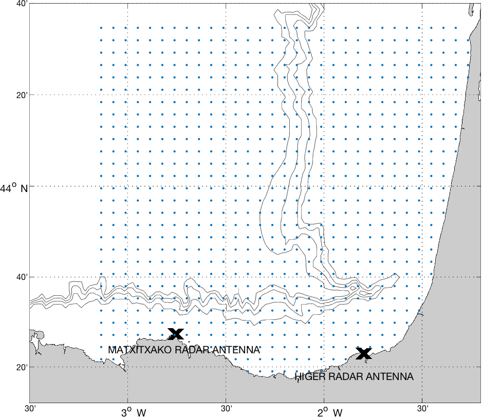
Figure 1Map showing the location of the two antennas (Matxitxako and Higer) of the BoB HFR systems. The grid points of the total HFR velocity field are plotted in blue.
3.1 OMA and DINEOF
Some methods, i.e., open-boundary modal analysis (OMA) and data interpolating empirical orthogonal functions (DINEOFs), are nowadays widely used to fill spatiotemporal gaps in HFR measurements. We briefly explain these two methods below.
Open modal analysis (OMA, Kaplan and Lekien, 2007) is based on a set of linearly independent modes that are calculated before they are fit to the data. These modes describe all possible current patterns inside a two-dimensional domain (taking into account the open boundaries and the coastline). The amplitude of those modes is then fitted to current measurements inside the domain. OMA considers the kinematic constraints imposed on the velocity field by the coast since OMA modes are calculated taking into account the coastline by setting a zero normal flow. Depending on these constraints they can be limited in representing localized small-scale features as well as flow structures near open boundaries. Difficulties may arise when dealing with gappy data, especially when the horizontal gap size is larger than the minimal resolved length scale (Kaplan and Lekien, 2007) or when only data from one antenna are available. In the case of large gaps, unphysically fitted currents can be obtained if the size of the gap is larger than the smallest spatial scale of the modes, since the mode amplitudes are not sufficiently constrained by the data (Kaplan and Lekien, 2007). This is why when using OMA it is recommended to reach a compromise between the number of modes used for spatial scales larger than the largest gap and a sufficient number of modes correctly representing the spatial variance of the original fields (knowing that the spatial smoothing increases as the number of modes decreases). For this work, we used the OMA modules in the HFR Progs MATLAB package (https://cencalarchive.org/ProgsRealTime/HFR_Progs/, last access: 20 August 2018) to process radial velocities into total currents. Setting a minimum spatial scale of 20 km, 85 OMA modes were built for the regular grid shown in Fig. 1. OMA is especially useful to obtain a solution in the baseline area (i.e., the area between the two radar antennas for which total currents cannot be computed directly from radial information) and has been used to provide fields to compute accurate trajectories (Hernández-Carrasco et al., 2018; Solabarrieta et al., 2016) and surface Lagrangian transport in coastal basins (Hernández-Carrasco et al., 2018; Rubio et al., 2018).
The data interpolating EOF (DINEOF) is an iterative methodology used to interpolate gaps or missing data in geophysical datasets (Alvera-Azcárate et al., 2005; Beckers and Rixen, 2003). The technique is applied to an N×M data matrix, where N is the size of spatial locations of the geophysical field, and M the time dimension of the data. Before the methodology is initialized, part of the initially non-missing data is removed from the data matrix and stored for cross-validation. Then anomalies are computed by removing the time mean at each location, and gaps or missing data are replaced by zero-value anomalies. At this point the data matrix is iteratively decomposed and rebuilt by means of an EOF analysis with a fixed number of EOFs. Values of originally missing gaps evolve through this iteration until convergence is met. By changing the number of EOFs, a set of such iterations is produced using a different number of EOFs in each repetition. The optimal number of EOFs is then deduced by cross-validation comparing the initially stored data with the different versions of the reconstructed data. Once the optimal number is deduced, the originally retained data are introduced back in the data matrix, and a final reconstruction is made using the optimal number of EOFs.
DINEOF was introduced by Beckers and Rixen (2003) and Alvera-Azcárate et al. (2005, 2007) in both univariate and multivariate forms. The method was initially applied to sea surface temperature and ocean color (Alvera-Azcárate et al., 2005, 2015; Beckers et al., 2014; Esnaola et al., 2012; Ganzedo et al., 2011; Volpe et al., 2012), but the technique has also been used for other variables like sea surface salinity (Alvera-Azcárate et al., 2016). The DINEOF Fortran code (http://modb.oce.ulg.ac.be/mediawiki/index.php/DINEOF, last access: 20 August 2018) was applied to the combination of radial currents from the two antennas. The MATLAB–Octave complementary sources provided with the Fortran codes are also used to produce cross-validation masks internally required by DINEOF, following the procedure proposed in Alvera-Azcárate et al. (2005). As in the case of the above mentioned DINEOF applications, spatial locations with more than 95 % of missing data are not included in the DINEOF reconstruction procedure to prevent a negative impact on the quality of the overall reconstruction. The covariance filtering option proposed in Alvera-Azcárate et al. (2009) was also applied, setting the number of iterations of the filter to 12. The number of retained EOFs was high for all experiments (a minimum of 75) independently of the considered gap scenario (see Sect. 4).
3.2 SOM
Here a new methodology has been developed in order to reconstruct HF radar velocity fields in the statistical framework of the self-organizing map (SOM) analysis. SOM is a powerful visualization technique based on an unsupervised learning neural network, which is especially suited to extract patterns in large datasets (Kohonen, 1982, 1997). SOM is a nonlinear mapping implementation method that reduces the high-dimensional feature space of the input data to a lower-dimensional (usually two dimensional) network of units called neurons. In this way, SOM is able to compress the information contained in a large amount of data into a single set of maps. The learning process algorithm consists of a presentation of the input data to a preselected neuronal network, which is modified during an iterative process. Each neuron (or unit) is represented by a weight vector with the number of components equal to the dimension of the input sample data. In each iteration the neuron whose weight vector is closest (more similar) to the presented sample input data vector, called the best-matching unit (BMU), is updated together with its topological neighbors located at a distance less than the neighborhood radius Rn towards the input sample through a neighborhood function (see Hernández-Carrasco and Orfila, 2018, for a schematic representation of the SOM). Therefore, the resulting patterns will exhibit some similarity because the SOM process assumes that a single sample of data (input vector) contributes to the creation of more than one pattern, as the whole neighborhood around the best-matching pattern is also updated in each step of training. It also results in a more detailed assimilation of particular features appearing on neighboring patterns if the information from the original data enables it to do so. At the end of the training process, the probability density function of the input data is approximated by the SOM and each unit is associated with a reference pattern, with a number of components equal to the number of variables in the dataset, so this process can be interpreted as a local summary or generalization of similar observations.
For typical remote sensing imagery, SOM can be applied to both the space and time domain. Here, since we are interested in the reconstruction of HF currents, we have addressed the analysis in the spatial domain. In this case the input row vector has been built using the radial velocity maps at each time, so each neuron corresponds to a characteristic radial velocity spatial pattern over the coverage area of the HFR. Since each step iteration has an associated time and location of the sample, we can obtain the time of a particular spatial pattern computing the BMU for each time, providing a time series of the corresponding spatial pattern.
From these ideas, we can deduce the following simple algorithm for reconstructing missing values in the HFR velocity field from the available HFR data.
- i.
Initialization (setup of the initial neural network). Each neuron (or SOM unit) has an associated weight vector, W, composed of random values of HFR radial velocities (called random initialization).
- ii.
Training process. Radial HFR velocity values at a time ti (Map of HFR velocities, U(x,ti)) are used as input vectors, , to iteratively feed the neural network. This process is divided into two phases: a rough training using a larger neighborhood radius Rn in the neighboring function and a fine-tuning training for small Rn. Note that Vi values are the HFR velocity maps with missing points.
- iii.
Spatial patterns. Once the training process has finished we obtain an ordered neural network of spatial patterns of radial HFR velocities (Vs). Now Vs does not include missing values.
- iv.
Identification of missing values (NaNs). Locate the position and time of the HFR velocity grid points with missing values (xm,tm).
- v.
Find BMU. Identify the most similar SOM spatial pattern to the HFR radial velocity map with missing values BMU(Vi(xm,tm)).
- vi.
Replace missing values. Once we have assigned the BMU we replace the points with missing values with values of the corresponding grid point of the BMU, obtaining the filled HFR velocity field, Vf, where
- vii.
Replace all NaNs. Repeat (v.) and (vi.) for all the points with missing values.
The ability of this method relies on the precision of identifying the proper BMU that accurately describes the missing dynamics. We try to optimize the algorithm by using as an input vector a concatenation of three maps of HFR velocities on three different dates. Thus we force the method to distinguish between three maps instead of one, avoiding the selection of a bad BMU, in particular when the HFR velocity map has a large number of missing points at time t0 and there are not enough points to compare with the SOM patterns. The input vector is thus . We have checked different values of Δt and found the best results when using Δt=4 h.
The initialization, training process and final output of the SOM algorithm have to be tuned in order to optimize the results and the computational cost by selecting particular control parameters. For instance, the optimal size of the neural network (number of neurons) depends on the number of samples and the complexity of the patterns to be analyzed. We choose the map size as [50×50], with 2500 neurons. Using different sizes, for instance [100×100], the spatial patterns are more detailed and more variability of patterns emerges. However, these new patterns make it difficult to find the proper BMUs for the specific date, creating considerable problems in accurately reconstructing the desired field in the missing points. The opposite happens using a reduced number of neurons: patterns are concentrated together in a few rough neurons without discriminating regions with different dynamical processes. We use a hexagonal map lattice to have equidistant neighbors and do not introduce anisotropy artifacts. Concerning the initialization, we opted for random mode. There are other initializations, i.e., based on a linear combination of the EOF modes of the HFR velocities, but all of them yield similar results. We choose random initialization since it is faster and missing data are accepted. For the training process we use the imputation batch training algorithm (Vatanen et al., 2015) adapted for data with missing values and a “Gaussian” type neighborhood function since this parameter configuration produces a good compromise between quantitative and topological error and computational cost (Liu et al., 2006). The neighborhood radius is chosen to vary from 20 to 0.1. Other values of the neighborhood radius have been tested without improving the results with the same computational cost. These SOM computations have been performed using the MATLAB toolbox of SOM v.2.0 Vesanto et al. (2000) provided by the Helsinki University of Technology (http://www.cis.hut.fi/somtoolbox/, last access: 20 August 2018).
Compared to conventional statistical methods like EOF and K-means, SOM is able to introduce nonlinear correlations and it does not require any particular functional relationship or distribution assumptions about the data, i.e., distribution normality or equality of the variance (Liu et al., 2006, 2016). SOM has been applied in a wide range of scientific disciplines. Among others, it has been used in climate sciences (Cavazos et al., 2002), genetics for DNA sequences (Nikkilä et al., 2002) and ecological sciences applications (Chon, 2011). In the physical and biological oceanography context SOM has also been used in several studies (Basterretxea et al., 2018; Charantonis et al., 2015; Hales et al., 2012; Hernández-Carrasco and Orfila, 2018; Liu and Weisberg, 2005; Liu et al., 2016; Richardson et al., 2003). However, to our knowledge, applications of SOM analysis to the reconstruction of HF radar velocity fields have not been addressed.
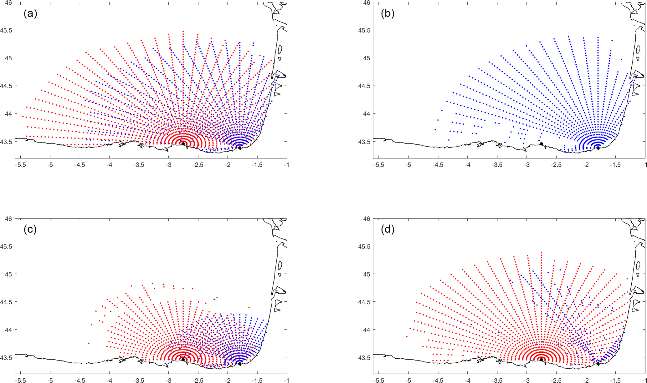
Figure 2Example of the four prototypes of KMA groups of gap distribution scenarios obtained from the KMA analysis applied to the HFR availability–absence matrix for 2014. Panel (a) represents a good data coverage scenario. Panel (b) accounts for the failure of one of the two antennas. Panel (c) characterizes a range decrease in both antennas. Panel (d) represents bearing coverage decreasing in one of the antennas. Matxitxako radials are plotted in red and Higer radials are plotted in blue (see Fig. S1 in the Supplement for the complete KMA results lattice).
The most common real scenarios for spatial gaps in HFR data are mainly represented by individual antenna failures, range and/or bearing reduction. The radio signal emitted by an HFR travels along and back through the ocean surface due to the conductivity of the ocean, and the current velocity is measured based on the Bragg scattering phenomena (Barrick et al., 1977) of the received signal. Any disruption to this process will result in gaps in the final data. Among the most common reasons to find spatiotemporal data gaps in radial (and total) components are adverse environmental conditions and/or electromagnetic problems such as the lack of Bragg scattering ocean waves, severe ocean wave conditions, the occurrence of radio interference or changes in the electromagnetic field in the vicinity of the antennas, which lead to invalid antenna patterns and calibration parameters. Additionally there is a permanent region between the antennas, the so-called baseline, in which the total currents cannot be computed in an accurate way. The baseline between two HFR sites is defined as the area where the radial components from the two sites have an angle of less than 30∘, so the total velocity vectors created from radial data within this area contain greater uncertainties. Normally, the solution in the baseline is not computed, so we observe a data gap in an area that is delimited by the rule of geometric dilution of precision (GDOP) (Barrick, 2002; Chapman et al., 1997) and the limits set to this quality control parameter in the processing of the data from radials to totals. The permanent spatial gap in the baseline is an issue than can be problematic for the assessment of dynamics near the coastal area between the antennas.
In order to characterize the most typical and realistic gap types observed in the Basque HFR system, a K-means classification algorithm (Hastie et al., 2009), henceforth KMA, is applied to the real radial data for 2014. Before applying the KMA, the radial data are converted to 1 or 0 values, depending on the availability or absence of data for each radial position, respectively. Then KMA is used to classify the dataset into a specified number of groups according to the similarity in the distribution of gaps exhibited in the HFR dataset (Hastie et al., 2009). The selection of the number of groups is done qualitatively, as proposed by Guanche et al. (2014). In our case we choose to keep 16 groups since this number facilitates the interpretation of the gap scenarios without losing the variability of the dataset (Fig. S1 in the Supplement). Groups 1, 5, 8, 9, 10, 14 and 15 are considered to represent a good data coverage; groups 4, 6, 7, 11 and 13 contain most of the common scenarios of spatial data gap; and finally, groups 2, 3, 12 and 16 show situations with no (or very few) data for any of the two antennas (no total currents can be produced). Examples of good coverage and gap scenarios corresponding to individual antenna failure, range reduction and bearing are shown in Fig. 2.
Since the goal of this work is to evaluate different gap-filling methodologies in real situations, the different groups representing observed gap types are used to introduce artificial gaps in April 2012, April 2013 and April 2014. Randomly generated spatial gaps are also included to cover different failures that are not related to the typical situations but could occur. For all the cases data gaps are introduced in 50 % of the time series. The proposed gap scenarios are the following: (A) bearing gaps generated by randomly distributing 10 of the elements of KMA group 6 (Fig. 2); (B) decreasing range generated by randomly distributing 10 of the elements of KMA group 4; (C) antenna failure (in this group failures of one of the two antennas were simulated by randomly removing data from one of the sites); and (D) random gaps (gaps were randomly introduced in the time series and randomly distributed over 30 % of the spatial HFR domain). K-means analysis shows that the situation associated with the patterns with a percentage of gaps greater than a 30 % is likely due to a failure of one of the two antennas than to other causes. This last scenario represents a situation in which data in selected locations have been removed (for instance after a quality control procedure based on a velocity or variance threshold, as recommended by QARTOD, 2015). Figures 3 and 4 show the temporal and spatial distribution of the percentage of coverage of the original data and the new dataset generated by introducing the previously described gaps to the original data.
These gap scenarios (from now on referred to as experiments A, B, C and D) are used to test the SOM, DINEOF and OMA gap-filling methodologies. For OMA, total maps are generated using OMA directly on radial data. For DINEOF and SOM, hourly radials are gap-filled first and then totals are generated using the same least mean square algorithm (spatial interpolation radius of 10 km) used to build the reference data series (i.e., from the reference radial files with no gaps).
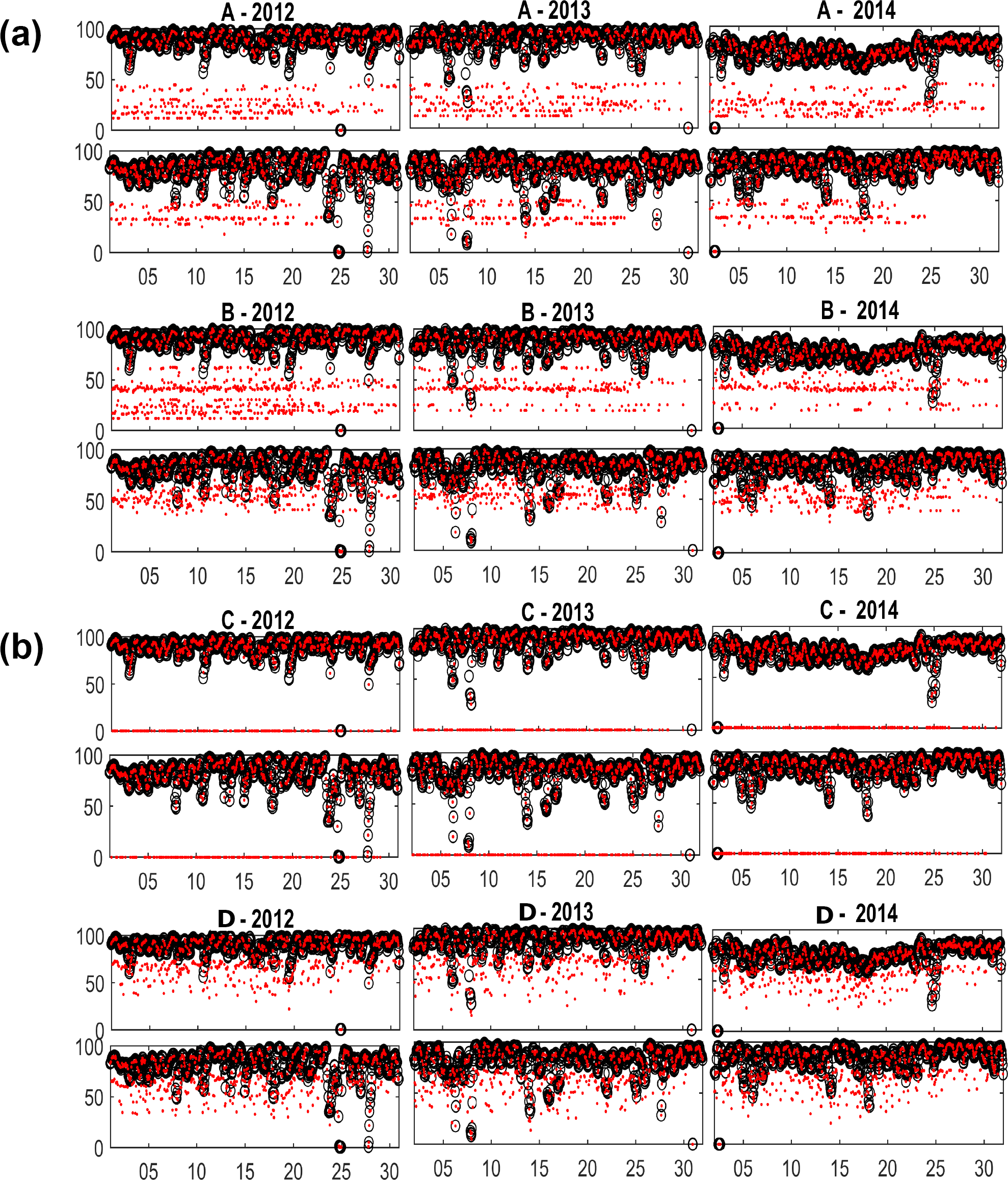
Figure 3Percentage of spatial coverage for each time step and experiment. Higer data are shown in the upper panels and Matxitxako data in the lower panels in all cases. Black circles represent the percentage of good data for the original fields. Red dots denote the percentage of good data for each experiment. The x axis is the time step of the time series for April 2012, April 2013 and April 2014.
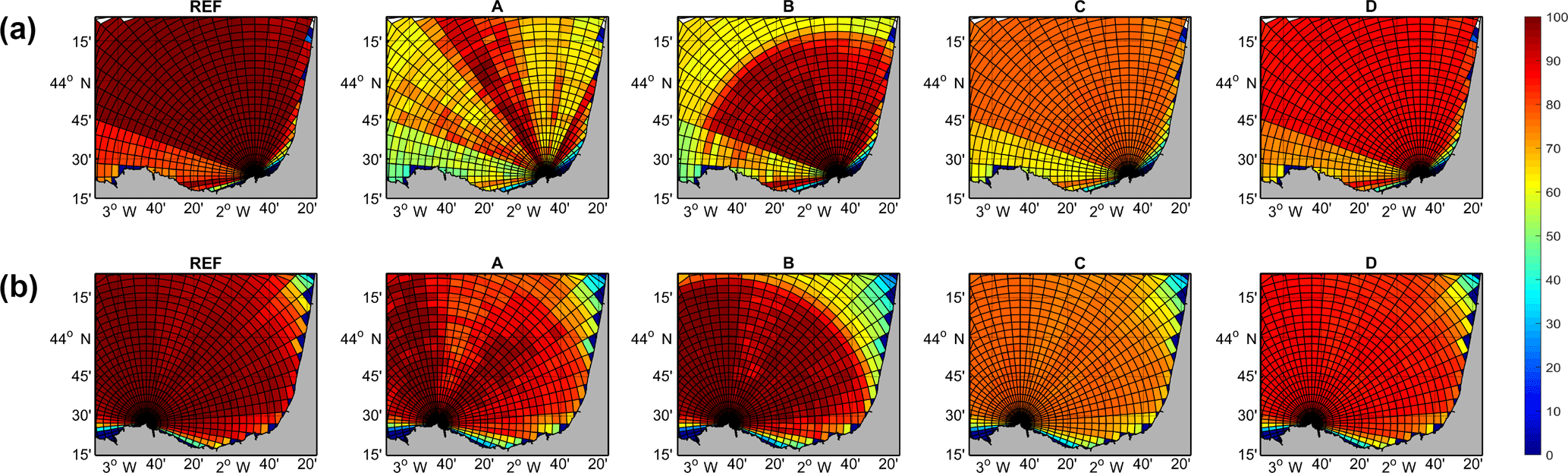
Figure 4Maps of temporal coverage (percent of the total number of hours in the 3-month period analyzed) for Higer (a) and Matxitxako (b) for the REF series and all the experiments.
In this study we compute different Lagrangian quantities using the HFR velocity field filled by the three different methods explained in Sect. 3: SOM, DINEOF and OMA. All the Lagrangian quantities, F (finite-size Lyapunov exponents, FSLE, and residence time, RT), computed from SOM are referred to as SOM-F. For instance, if we compute the FSLE from the SOM reconstructed HFR currents, it is referred to as SOM-FSLE. The same applies to DINEOF and OMA. We use as the reference field the original HFR velocity field in the periods when it is complete. This complete HFR dataset is named REF, and, for instance, REF-FSLE refers to FSLE computed from REF.
We use conventional statistical metrics to measure differences between gap-filled and observation data to quantify methodology skill: absolute relative error (ARE), mean bias (MB) and root mean squared (RMS) error. By denoting a set of reference observational values as R, denoting the corresponding data obtained from the filled velocity field as G, using brackets to denote the mean of the set and a prime to denote variations from the mean, i.e., , these error metrics are defined as
where N is the number of pixels in the velocity field.
6.1 Eulerian comparison
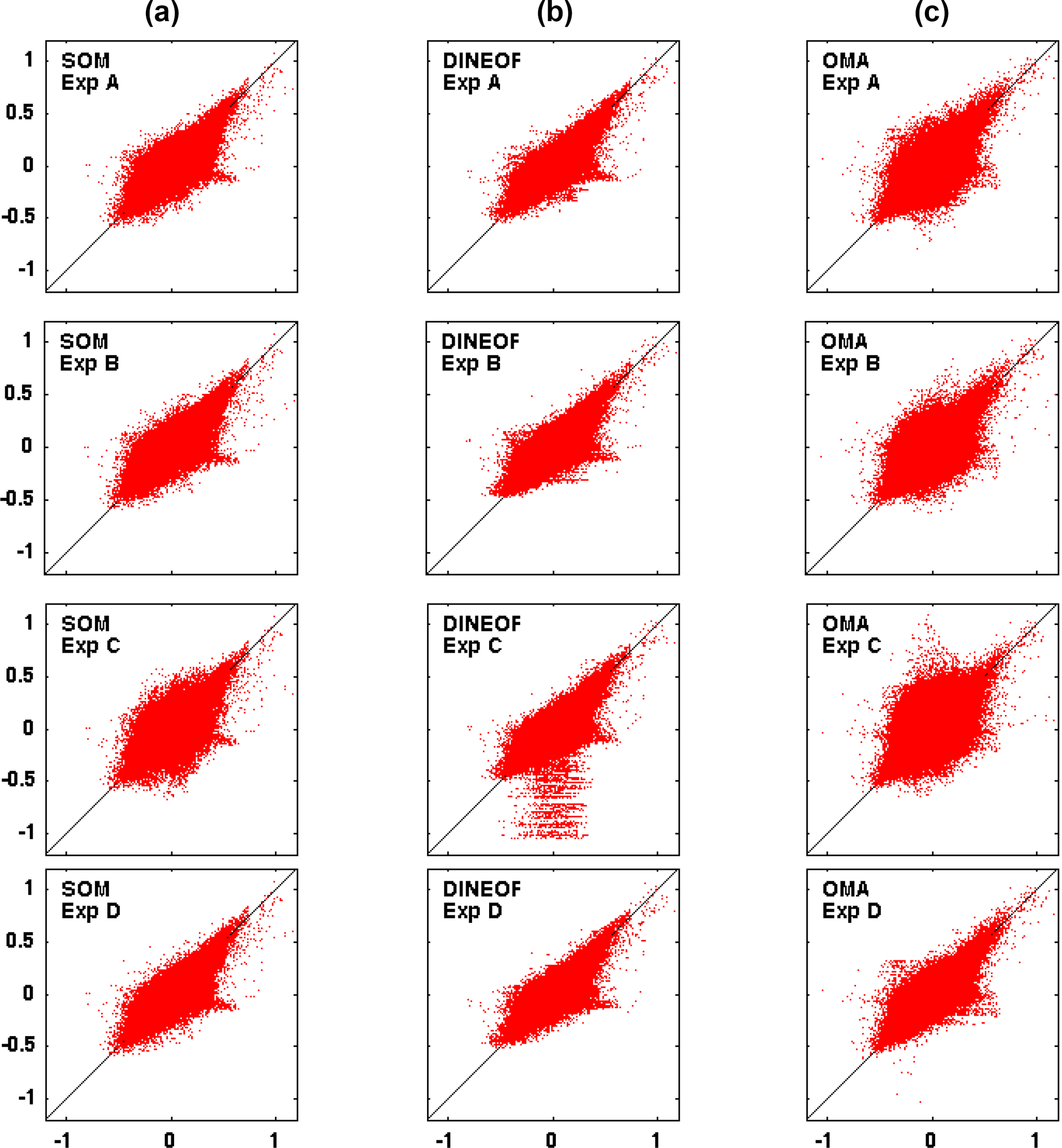
Figure 5Scatterplot of the SOM (a), DINEOF (b) and OMA (c) reconstructed zonal velocities vs. observations for the four experiments (rows).
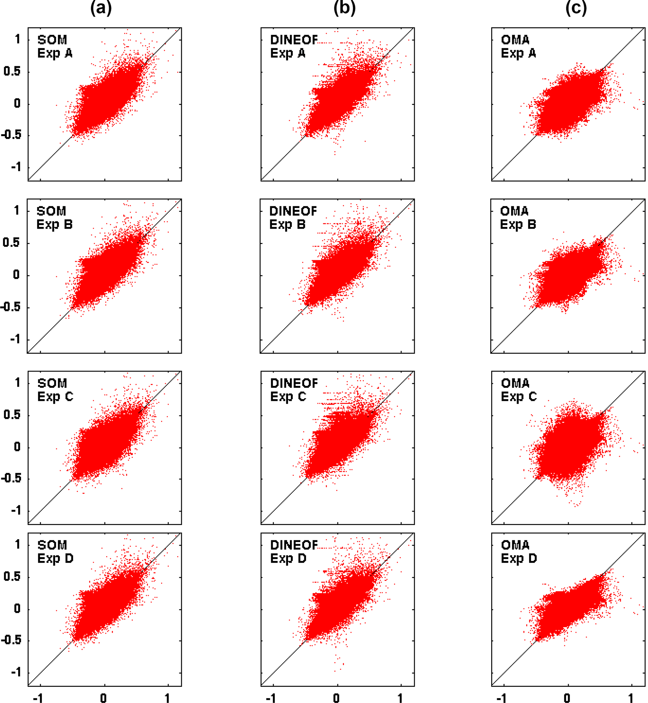
Figure 6Scatterplot of the SOM model (a), DINEOF (b) and OMA (c) reconstructed meridional velocities vs. observations for the four experiments (rows).
Scatterplots of zonal (u) and meridional (v) velocities reconstructed by the three models vs. the reference field and for the four experiments are shown in Figs. 5 and 6, respectively. In the case of OMA the cloud of points is, in general, wider with more points separated from the baseline. In general the behavior of the SOM and DINEOF methods is very similar in terms of RMS, BIAS and R2 as displayed in Tables 1 and 2 for the u and v component of the velocity, respectively. Although SOM tends to underestimate currents and DINEOF to overestimate, OMA shows the worst reconstruction, especially for experiment C. It is worth noting that models behave similarly for component u and component v for all experiments. The lowest mean error is found for experiment D with values of 0.36, 0.35 and 0.38 for SOM, DINEOF and OMA, respectively, and the highest for experiment C with values of 0.43, 0.38 and 0.57 for SOM, DINEOF and OMA, with antenna failure as the worst-case gap scenario to be properly reconstructed. In particular, the scatterplot of reference vs. reconstructed zonal velocities from DINEOF in the case of the experiment C (Fig. 5 second column, third row) shows many points out of the main cloud. It suggests that the gap scenario C, in which a very small number of observations is available (failure of one antenna), is the most difficult gap scenario for the DINEOF methodology. Typically a 5 % minimum threshold of available data is used in most DINEOF applications reported in the literature to accept a candidate for a potential reconstruction (for instance, a gappy satellite image or an hourly HFR current field). As described in Sect. 3, such a threshold is also applied here as a preprocessing step before the technique is applied. The spatial field of the missing antenna is reconstructed using available data from the other antenna, as well as data from previous and subsequent time steps. Although in general the field might be acceptably reconstructed, it seems that some parts of the HFR image are not properly reconstructed. This result suggests that DINEOF should not be considered in situations represented in scenario C, especially when the antenna failure is persistent over time. Relative errors are slightly lower for DINEOF than for SOM but with more outliers as shown in Figs. 5 and 6.
Table 1Root mean square (RMS) error , mean bias (MB) and correlation coefficient (R2) of the zonal velocities (u) obtained using reconstructed HFR field from the three methodologies and for the four experiments with respect to the zonal velocities derived from the reference HFR currents.
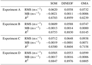
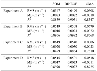
Table 2Root mean square (RMS) error, mean bias (MB) and correlation coefficient (R2) of the meridional velocities (v) obtained using reconstructed HFR datasets from the three methodologies and for the four experiments with respect to the zonal velocities derived from the reference HFR currents.
6.2 Comparison of trajectories
Synthetic trajectories are computed by advecting particles in the original HFR velocity field (reference trajectories) and also in the OMA, SOM and DINEOF gap-filled currents. A total of 868 particles are initially uniformly distributed over the HF radar grid with an initial distance between particles of 5 km. Lagrangian particles are released every hour from 2 to 26 April 2012, 2013 and 2014 and advected during 72 h. Trajectories are computed using a fourth-order Runge–Kutta integration scheme and a bilinear interpolation of the gridded velocity field in space and linear in time. The mean distance of separation (D) between particle trajectories advected by the reference velocity field and by the reconstructed current fields averaged over all pairs of trajectories is plotted against time for each experiment in Fig. 7. After 10–15 h, differences in D start to be visible in all the cases. In all the experiments, DINEOF and SOM show lower separation distances and a similar behavior, while the OMA method shows the highest errors, in particular in the case of failure of one of the antennas (experiment C). In this case OMA capability to fill gaps is limited (as discussed in Kaplan and Lekien, 2007) and the effects can be noticed from the beginning of the trajectory simulation. The DINEOF and SOM methods show similar results, with separation distances around 1 km after 24 h of simulation and 3 km after 72 h. Values of D for SOM are slightly smaller in all of the experiments. In contrast, this distance reaches values of 5 km after 24 h in the case of OMA. The values of D obtained in our computations after 24 h of simulation are smaller than those reported in Molcard et al. (2009), Bellomo et al. (2015) and Kalampokis et al. (2016) for separation distances between real and virtual drifter trajectories. It is important to keep in mind that in these experiments the trajectories are calculated with data from different sources (HFR and drifters) and different samples (spatial resolution), which are collected in a different region (Mediterranean Sea). However, the fact that we obtain smaller values of D is an indication of the high performance of the three methods, with better results observed for the SOM method compared with OMA and DINEOF.
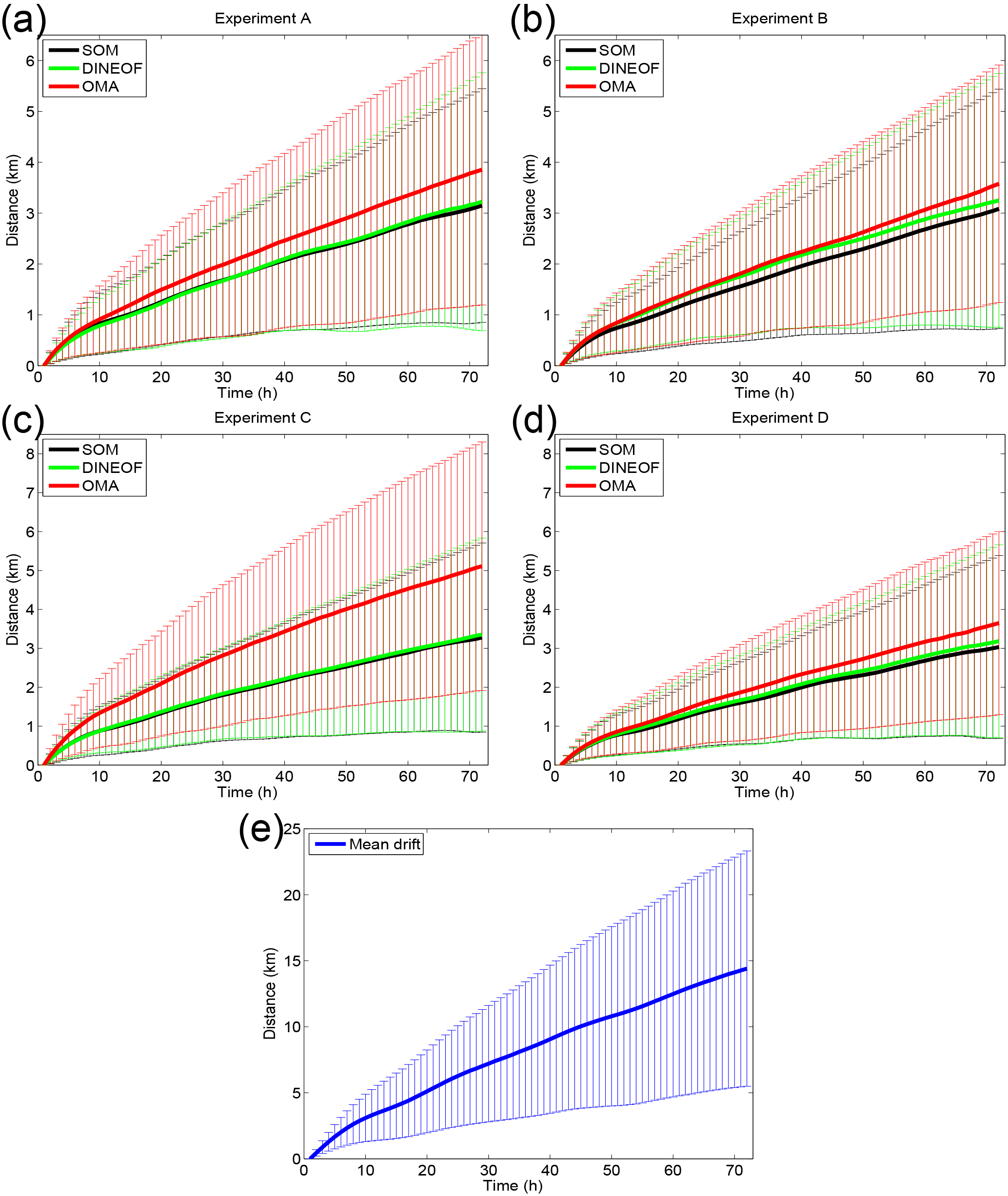
Figure 7Separation distance between particle trajectories advected by the filled HFR velocity field and by the reference velocity field as a function of time and averaged over all the pairs of trajectories. Different limits in the vertical axis of the figure have been used for a better data representation. The error bar is the confidence interval (1 standard deviation) of the spatial average of D(t).
The spatial distribution of separation distances between real and simulated trajectories has also been analyzed in order to detect any anisotropy in the differences between them (Fig. 8). The results show the same behavior of the temporal separation distances between the different methodologies and experiments, but DINEOF and SOM yield better results than OMA. It is worth noting that OMA capability decreases in the western part of the study area in all the experiments, especially when there is a failure in one of the two antennas (experiment C). It is also noticeable that the time average of the separation distances is smaller in this experiment for DINEOF than for SOM. In general, all the methodologies show lower separation distances in the central and eastern part of the study area than in the western part, which demonstrates that the performance of the methodologies has spatial variations and is not uniform.
6.3 Lateral stirring analysis
Furthermore, we analyze the effect of the different gap-filling methodologies on the FSLE computations. FSLE was originally introduced in dynamical system theory to characterize the growth of non-infinitesimal perturbations in turbulence (Aurell et al., 1997) and to characterize flows with multiple spatiotemporal scales (Boffetta et al., 2000; Lacorata et al., 2001). In addition, FSLE can be used to unveil dynamical structures, called Lagrangian coherent structures (LCSs), thereby identifying fronts, eddies and jets (Hernández-Carrasco et al., 2011), as well as studying the flow stretching and contraction properties in geophysical data (Hernández-Carrasco et al., 2012; Joseph and Legras, 2002; Lipphardt et al., 2006; Shadden et al., 2009).
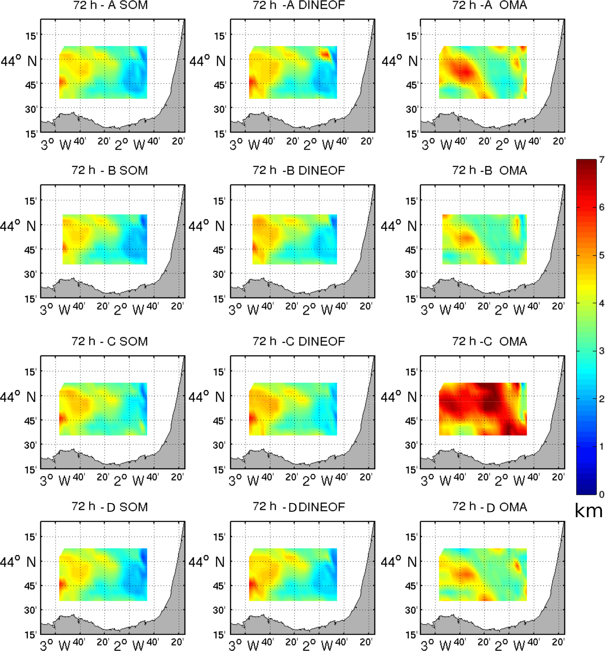
Figure 8Time average of the separation distance between trajectories computed from the filled HFR using the three methodologies and reference HFR velocities initiated in the same pixel.

Figure 9Comparison of scale-dependent FSLE curves computed from the different filled HFR velocities averaged over 240 virtual particle-pair deployments homogeneously distributed through April 2012, 2013 and 2014. (a) Experiment A, (b) experiment C.
The contribution of the scales captured by HFR in ocean surface dynamics can be analyzed by computing particle dispersion at different spatial scales, δ (Boffetta et al., 2000; Corrado et al., 2017; Haza et al., 2010), using the following equation for FSLE:
where 〈τ(δ,rδ)〉 is the time (τ) needed for the initial perturbation δ (separation of the initial pair of particles) to grow rδ averaged over all the pairs of particles for every initial perturbation δ and a fixed threshold rate, r. A small value, r<2, allows for the capturing of the relative dispersion driven by small coherent features, but r should not be close to 1 to avoid aliasing problems associated with the time step of particle advection at small scales (Haza et al., 2008; Lacorata et al., 2001). FSLE is a measure of relative dispersion for which the spatial variable is the independent variable.
We evaluate how the gap-filling methodologies impact the dynamical scales captured by the HFR. Figure 9 shows the averaged FSLE curves obtained from the three methodologies in two of the four experiments. The other experiments yield similar results. In all of them, λ(δ) is not constant over the range of scales covered by the HFR (scale dependent). In the REF case the best fit of the averaged FSLE curve shows a slope of −0.50 and a correlation coefficient, R2, of 0.97. This indicates that the average scaling law of relative dispersion over the scales from 6 to 40 km is associated with a turbulent dispersion for flows with a k−2 type of spectrum (Capet et al., 2008; Klein et al., 2008), suggesting that ageostrophic velocities and frontogenesis are contributing to lateral dispersion at these scales (Callies and Ferrari, 2013). This means that the separation rate is controlled by structures with sizes comparable to the separation itself, and therefore the dispersion regime is local. The slope of the FSLE curve derived from the REF HFR velocity field is in agreement with previous modeling studies, with a slope similar to those derived from surface synthetic drifter trajectories integrated by high-resolution numerical simulations (Choi et al., 2017). It further reinforces the fact that the velocity field of the HFR is adequate to study small-scale dynamics.
Comparing the FSLE slopes obtained from the three gap-filling methodologies with the REF HFR velocity field we find that the SOM methodology yields the most similar values, with slopes of and R2 greater than 0.96 for all the experiments, followed by the DINEOF with slopes of and R2 also greater than 0.96 for all the experiments. Finally OMA yields the largest differences with slopes between −0.27 and −0.30 and high R2 (greater than 0.94). The SOM-FSLE slopes are slightly steeper than the REF-FSLE, suggesting that this methodology could introduce noise in the reconstruction of the data. On the other hand, DINEOF-FSLE slopes are slightly flatter than the REF-FSLE, which could be produced because this methodology smooths the velocity field or because it favors larger scales as captured by EOFs. However, OMA-FSLE slopes are clearly flatter than the REF-FSLE. In this case, λ(δ) is almost constant over the range of scales (scale independent), the separation of particles is almost exponential with a constant rate and we have a nearly exponential regime. In this regime the relative dispersion is nonlocal, indicating that not only small-scale processes govern the dispersion but also larger structures. This result suggests that OMA has a strong smoothing character, removing small features from the velocity field, as reported in previous Eulerian studies (Kaplan and Lekien, 2007).
Compared with other observational studies using HFR the λ obtained from our computations is 1 order of magnitude smaller than the one reported in Haza et al. (2010) (λ=4 to 7 days−1 for δ<1 km) computed from VHF radar with 300 m of spatial resolution in the Gulf of La Spezia. This is expected when comparing their scales of interest (0.1–1 km) against our range of resolved scales (5–25 km) (Corrado et al., 2017). Hernández-Carrasco et al. (2018), using HFR velocities at 3 km of resolution in the Ibiza Channel, reported larger values of λ (between 0.6 and 0.2 days−1) at spatial scales between 3 and 30 km following a Richardson slope. Other studies based on drifters in the Gulf Stream (Lumpkin and Elipot, 2010), the Gulf of Mexico (Poje et al., 2014) and the Mediterranean Sea (Griffa et al., 2013; Schroeder et al., 2011) have found higher values of λ(δ) at these scales. Regional differences and possible observational biases could explain these discrepancies in FSLE values. For instance, differences in the topographic boundaries and/or the presence of coastal jets, tidal currents or particular wind regimes can influence the dynamics affecting transport processes at the coastal sea surface.
In general the λ values obtained for the three methodologies and for all the experiments are smaller than for REF, in particular when OMA velocities are used. At the smallest scales studied here (5–15 km) SOM-FSLE is the most similar, and at larger scales DINEOF-FSLE and OMA-FSLE values are closer to REF-FSLE.
Next we analyze the effect of the reconstructed velocities on the LCS. FSLE is used to obtain the LCS by computing the minimum growth time of particle-pair separations from δ to rδ among the four neighbors for each position in order to obtain an FSLE map. In this case, r has to take large values (r≫2) to adequately distinguish regions of extrema in the FSLE field. Note that in this case the average over the pair of particles in Eq. (6) is omitted.
First we compare some snapshots of the LCS derived from the three reconstructed HFRs in order to see differences in the dynamical structures (Fig. 10). We only show LCS from two experiments, A and C, since the results obtained in experiments B and D are similar to those of experiment A. The computed Lagrangian flow structures look rather the same in the case of SOM and DINEOF, despite the large number of missing points reconstructed in both experiments. This is also confirmed by computing the histograms of the FSLE (not shown), which turn out very similar. This is likely due to the averaging process along trajectories performed to compute the FSLE, which tends to remove possible errors introduced in the reconstructed velocity fields (Hernández-Carrasco et al., 2011). FSLE is robust against the gaps in the HFR velocity field. On the other hand, OMA is the most affected methodology regarding LCS computations. Even if not very different, one can see some discrepancies in the shape and the location of OMA-LCS with respect to the REF-LCS, as happens in experiment C (Fig. 10b).
The time evolution of the spatial average over the HFR domain of the absolute relative error (ARE; Sect. 5) of the attracting LCS computed from the reconstructed velocity fields with respect to the REF-LCS is plotted in Fig. 11. A common characteristic for the three methods is large values of ARE during early April 2012 and middle April 2014 for all the experiments, in agreement with the time periods with the largest number of missing values. Comparing the methods one can see that the relative error is mostly greater for the case of OMA and for all the experiments, in particular during the second half of April 2012 and the middle of April 2013 and 2014. All the methods are more affected by the antenna failure simulated in experiment C, in accordance with the Eulerian comparison.
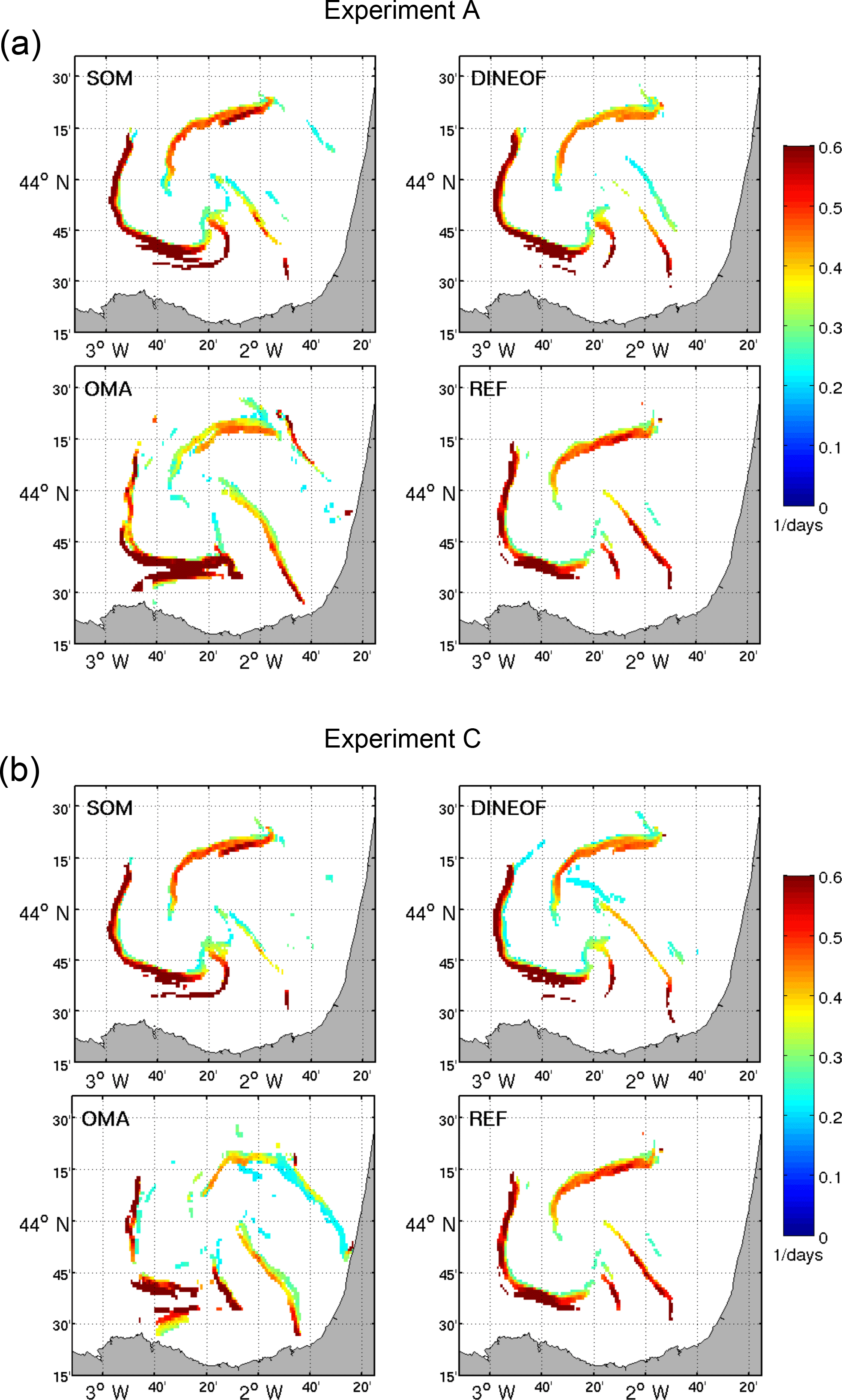
Figure 10Snapshots of attracting LCS computed from the three filled and the reference HFR currents for experiment A (a) and experiment C (b) corresponding to 11 April 2014, 00:00 UTC.
.
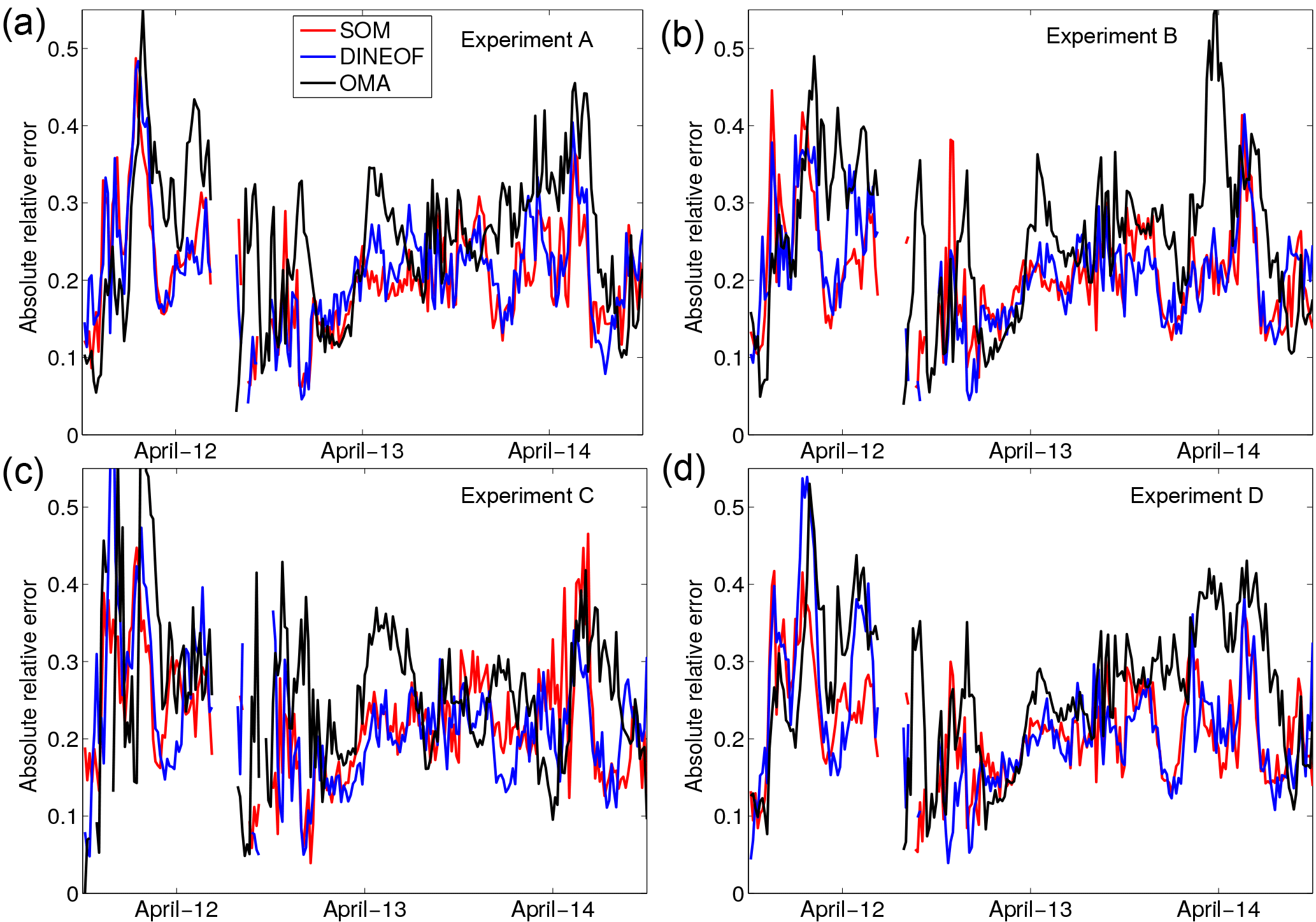
Figure 11Time series of the spatial average of the pixel-by-pixel absolute relative error of the LCS computed from the three filled HFR velocities with respect to LCS obtained from the reference velocity field.
Further analysis is conducted by performing a regional characterization of the impact of the gap-filling methods on the LCS looking at the spatial distribution of the time-averaged values of ARE (Fig. 12). One can appreciate that points with accumulated large errors are located in the same regions for SOM and DINEOF, i.e., in the southern area of the BoB HFR domain, and that these regions are the same for the four experiments (near the southern coastline). In addition to possible smoothing or noise, a discrepancy in the location of LCS with respect to the REF-LCS could explain the large values of the errors. In the case of OMA, additional regions with large errors are distributed all over the BoB HFR domain.
Finally, we quantify the difference between the LCS computed from the filled velocities and the REF-LCS by computing the spatial and temporal mean of the relative error defined in Eqs. (3) and (4) over all the LCS maps. We summarize in Table 3 the results of these computations. The most significant result is that ARE values are similar for SOM and DINEOF and for all the experiments (around 0.21), being in general slightly smaller for the case of SOM. The largest ARE is found for OMA-LCS in experiment C with the worst-case gap scenario affecting LCS, with a value of 0.27. The values of MB show that in general the LCSs are slightly overestimated. Only in experiment C are the values of OMA-LCS underestimated.
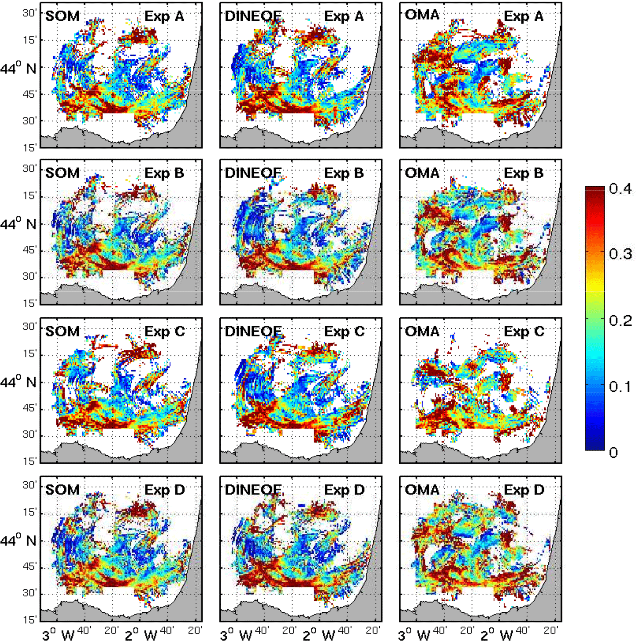
Figure 12Maps of the time average of the pixel-by-pixel absolute relative error of the LCS computed from the three filled velocity field with respect to LCS obtained from the reference currents. White denotes points at which LCSs have not been identified.
Our results show that even when a large number of pixels is missing the FSLEs still give an accurate picture of oceanic transport properties, and the velocity field filled by the three methods analyzed does not introduce artifacts in the Lagrangian computations.
6.4 Residence times
Another Lagrangian quantity suitable to describe transport process is residence time (RT) (Buffoni et al., 1996; Hernández-Carrasco et al., 2013; Lipphardt et al., 2006). RT is commonly used to characterize the fluid interchange between different oceanic regions and is defined as the interval of time that a particle remains in an area before crossing a particular boundary. In the calculation of RT particles are initially located on the grid points of the HFR velocity field and are integrated in time during 14 days. We consider only 14 days owing to the short period of available data without missing values (REF field). In these computations we assign the maximum possible value of RT (14 days) to the particles that remain in the area without crossing the preselected boundary after the 14 days of integration.
Table 3Mean absolute relative error (ARE) and mean bias (MB) of the LCS obtained using reconstructed HFR velocities from the three methodologies with respect to the REF-LCS for the four experiments.
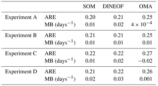
As done for the LCS, a first comparison is performed looking at the spatial distribution of RT obtained from the three different filled HFR datasets. In general, RT maps from the three methodologies are similar to the REF-RT (maps of RT obtained from the reference HFR velocity field). As an example, Fig. 13 shows two maps of RT for experiments A and C corresponding to 4 April 2013, 18:00 UTC. In this figure we color the initial position of particles in the BoB according to the time they need to escape from the HFR domain. Regions with particles with short residence times are shown in cyan–blue, and initial positions of particles having longer residence times are indicated in light brown. Again these two experiments are representative for the other experiments since experiments B and D produce an RT spatial distribution similar to that shown for experiment A (Fig. 13a). As it can be appreciated, the spatial patterns of RT obtained from the filled HF radar velocity fields are similar to the REF-RT in experiment A (and also for experiments B and D, not shown). Only some differences are found in OMA-RT maps compared to REF-RT for experiment C, as can be seen in Fig. 13b (OMA panel) with higher values of RT in the west and southeast regions of the HFR domain.
To further analyze the periods when the gap-filling methods introduce more errors in the RT computations we plot in Fig. 14 the time series of the spatial averages of the ARE of the RT. Most of the reconstructed derived RT values approximate REF-RT values, with ARE smaller than 0.2 along the time series. It can be seen that, except at the beginning of April 2012, values of ARE for OMA-RT are larger than SOM-RT and DINEOF-RT, in particular at the end of April 2012 and in the middle of April 2013 and April 2014. Again, experiment C turns out as the more critical situation for gap distribution to be reconstructed, reaching the largest values of ARE (around 0.25).
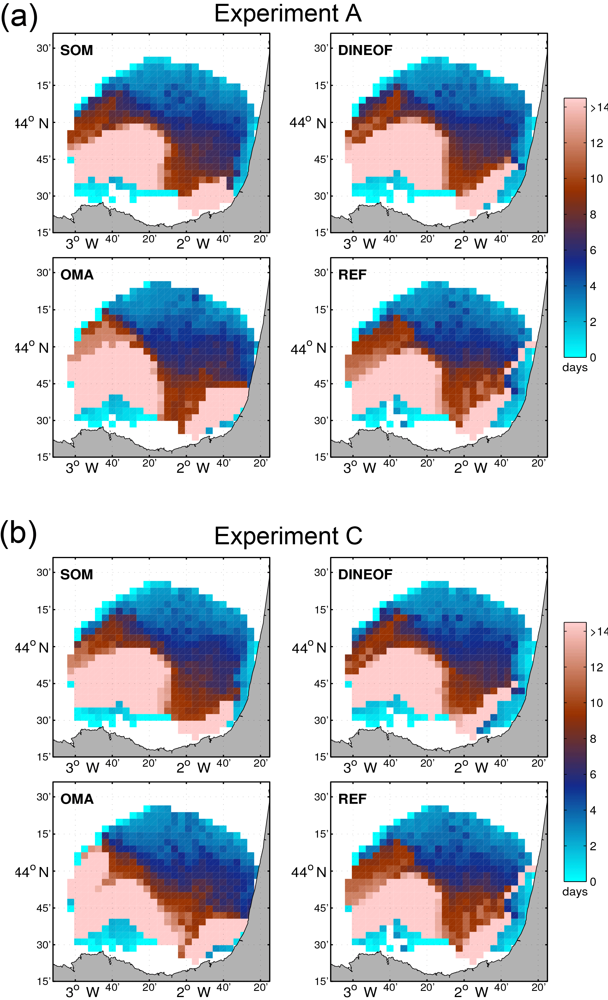
Figure 13Snapshots of RT computed from the three filled velocity fields and the reference HFR currents for experiments A and C corresponding to 4 April 2013, 18:00 UTC.
Figure 14Time series of the spatial average of the pixel-by-pixel absolute relative error of the RT computed with the reconstructed velocities with respect to the REF-RT.
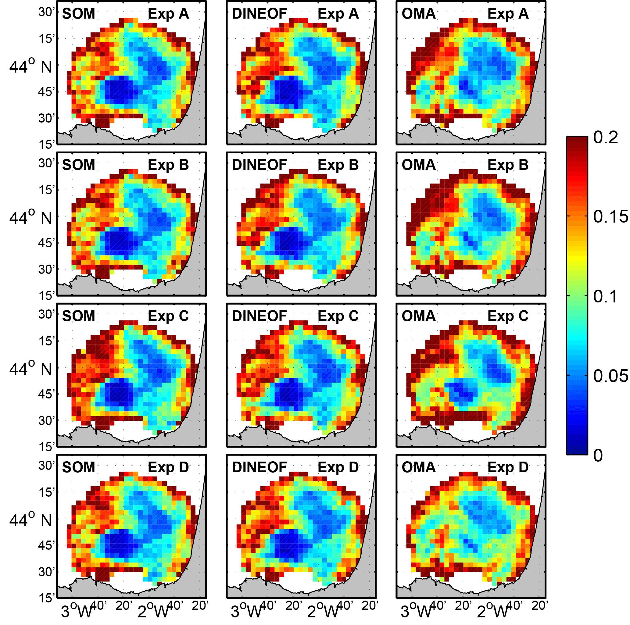
Figure 15Maps of the time average of the pixel-by-pixel absolute relative error of the RT computed from the three filled velocities with respect to RT obtained from the reference velocity field.
In order to reveal regions where the effect of the reconstruction on the RT is higher we compute the time-averaged relative error for all experiments (Fig. 15). This figure shows that, as for the LCS comparison, regions of accumulated errors are the same for SOM and DINEOF and this spatial distribution is quite similar for the four experiments. OMA shows different regions with large errors, being the method with the greatest number of pixels with large error. A common feature is that the three methods yield large errors near the southern coastline and in the west and northwest area of the HFR domain. It suggests that the three methods remove some dynamical features in this region. For points located in central regions (around 2∘ W and 44∘ N) values of RT derived from the reconstructed velocities better approximate the REF-RT values. The greater availability of data over this region could explain this agreement in the RT computations.
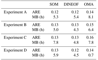
To finish this section, we summarize in Table 4 the results of the ARE and ME of RT averaged over all the RT values. Although ARE is slightly greater in the case of OMA than using SOM and DINEOF, in general these errors are low in all cases, with 0.16 as the maximum ARE obtained over all the experiments. The absolute error is smaller for SOM and DINEOF (between 0.12 and 0.13 for both cases) and slightly larger for OMA (between 0.13 and 0.16). Furthermore, the AREs for SOM-RT and DINEOF-RT are quite identical. In all cases the MBs are positive, meaning that RTs are overestimated. The largest values of MB are found, on average, for OMA-RT (MB ranging from 0.7 h for experiment D to 8.1 h for experiment A), followed by SOM-RT (MB ranging from 5.0 h for experiment B to 7.8 h for experiment C) and finally by DINEOF-RT (MB ranging from 4.3 h for experiment B to 5.4 h for experiment A).
We have investigated the performance of HFR gap-filling methodologies by studying the reliability of some basic Lagrangian metrics for the assessment of coastal dynamical properties when they are computed using reconstructed velocity fields. A sensitivity test has been carried out through four experiments including the most common scenarios of data gaps observed in HFR systems, i.e., hardware failures, communication interruptions, particular environmental conditions affecting the detection of the signal and sea state.
Table 4Mean absolute relative error (ARE) and mean bias (MB) of the RT obtained using reconstructed HFR velocities from the three methodologies with respect to the REF-RT for all the experiments. A total of 156 240 RT values are used in the computations.
In contrast to other comparative studies of different gap-filling methodologies based on Eulerian differences (Fredj et al., 2016; Yaremchuk and Sentchev, 2009), we have focused on the propagation of the errors introduced in the reconstruction of the velocity fields through Lagrangian metrics. We found that the relative errors (up to 43 %, 38 % and 57 % in the case of the SOM, DINEOF and OMA methods, respectively, in the worst gap scenario corresponding to one antenna failure) are reduced in the Lagrangian diagnosis. The largest errors for the LCS computations are up to 22 %, 22 % and 27 % and for the RT up to 13 %, 13 % and 16 % obtained with the SOM, DINEOF and OMA reconstructed velocities, respectively.
The four experiments based on different groupings of missing values demonstrate that even for spatially severe and persistent gaps, the Lagrangian diagnoses obtained from FSLE fields and RT are robust representations of the surface dynamics in coastal basins. Our results show that even when a large number of pixels is missing the FSLE computations still give an accurate picture of oceanic transport properties. The velocity fields filled by the three methods analyzed do not introduce artifacts in the Lagrangian computations. The robustness of the Lagrangian diagnoses against errors in the velocity data could explain the low relative error in the FSLE and LCS computations from the reconstructed velocities (Hernández-Carrasco et al., 2011).
While DINEOF presents the lowest errors in the Eulerian frame, SOM is the method with the lowest errors in the trajectory, LCS and RT computations. The DINEOF and SOM reconstruction methods are based on patterns of the velocity field extracted from statistical concepts. These methods strongly depend on the number of modes and/or neurons used in the reconstruction. The greater the number of modes and/or neurons, the less smoothed the pattern will be. However, even when using a large neural network or number of modes, these methods are prone to filter the velocity field, removing some small-scale dynamical features, and in some cases the resulting patterns are a smoothed representation of the real dynamics. DINEOF and SOM also depend on the choice of the modes or patterns. This could explain the large number of points out of the main cloud in the scatterplot shown in Fig. 5 for DINEOF in experiment C. These outliers can propagate the error in the computations of trajectories, explaining the difference between the Eulerian and Lagrangian comparison of the DINEOF and SOM methods. In the SOM methodology the fact that each neuron is composed of velocity fields at three different times could increase the probability of using a more suitable pattern for the reconstruction, in particular in the cases in which there is a large number of missing points (i.e., experiment C, failure of antenna).
On the other hand, OMA is a geometrical approach that uses a combination of irrotational and incompressible field configurations and the spatial shape of the HFR domain to decompose the HFR velocity field. This technique also depends on the choice of the modes and the number of modes. In general, since only a finite number of modes is computed, an arbitrariness is introduced in the selection of the modes; the real velocity is projected into a subspace of modes that are either tangent to the coastline or to the open boundary. Using a small number of modes could affect the results of the reconstruction, obtaining a velocity field far away from the HFR data but with very simple features. In situations in which the flow patterns are simple and quasi-permanent, the use of a few modes is able to capture these main features. In contrast, if a large number of modes is used, the reconstructed field matches the HFR data, but the data are not sufficiently filtered and smoothed, introducing some dynamical features or even artifacts, which may not exist in the real flow. In our case, the coastline in the area of the HFR coverage is relatively large, originating an increase in the number of modes tangent to the coast to the detriment of the OMA open-boundary modes and therefore conditioning the resulting inferred velocity field. As explained in Sect. 3, the constraints applied in OMA can limit the representation of localized small-scale features and flow structures near open boundaries. As discussed in Kaplan and Lekien (2007), difficulties may arise when the spatial gap size is larger than the smallest resolved length scale, explaining why weaker results are obtained when only data from one antenna are available. The study of the effect of individual sources of errors on the reconstruction is not trivial and depends on the coherence and persistence of the dynamical features as well as on the full knowledge of the dynamical scales involved in the tracer motion. Further analyses are needed to answer these questions, but this is out of scope of this paper and should be addressed in future studies.
In general, regions less affected by missing points are located in the middle of the HFR domain. The large coverage of data can explain this spatial distribution. Moreover, large errors are concentrated in the western part of the HFR domain, likely induced by the high variability of the flow in this region, increasing the effect of velocity error on the trajectories. The low number of gaps in the central part of the HFR domain in experiment B and the separation of the missing points randomly distributed in experiment D can explain the similarity in the Lagrangian diagnosis obtained in these experiments for the three gap-filling methodologies. Experiment C, simulating the failure of one of the two antennas, is the worst-case gap scenario, obtaining the largest errors in all the Lagrangian computations according to the errors found in the Eulerian comparisons.
The time period selected (April) represents the dynamical conditions during springtime. This is a transition period between the winter (when the persistent Iberian Poleward Current dominates) and summer when low energy and stable conditions are observed (Solabarrieta et al., 2014). Applying the methodologies over this period characterized by high dynamical variability allows us to avoid specific circulation patterns, ensuring the application of the results to other areas. However, analysis in different regions and periods is required to corroborate this statement.
Concerning the temporal distribution of gaps, we have introduced gaps in 50 % of the time period, which is much higher than the 10 %–20 % failures accepted in a well-functioning system. Nevertheless, this study is more focused on the spatial gaps and further analysis should be done to analyze the limit of applicability of each method regarding the temporal horizon.
All the results reported in this study cannot be extended to HFR systems working at different frequencies and resolutions. HFR working at different frequencies captures dynamical features at different scales that could be altered during the reconstruction process. Further studies using data from different HFR systems and regions characterized by different dynamical conditions should be performed to address this question. For instance, some SOM and DINEOF modes used in the reconstruction are smoothed representations of the real dynamics and they could remove some small-scale dynamical processes. However, these results are illustrative of the high performance of the gap-filling methodologies in providing reliable HFR velocities for a Lagrangian assessment of ocean coastal dynamics.
Contrary to SOM and, to a lesser extent, to DINEOF, one of the main advantages of using OMA is that this method does not need long time series of data and therefore it can be used immediately after installing the HFR system. Also, OMA allows for the reconstruction of total velocities in areas of large GDOP error, which also represents an advantage since it enables a larger spatial coverage. DINEOF also has the advantage of not requiring long training datasets and of not having subjective parameters. On the other hand, SOM is able to introduce nonlinear correlations in the computation of the patterns.
These experiments also show that the developed SOM methodology is suitable to properly encode the dynamical patterns present in turbulent flows. This is a very promising result and opens up new possibilities for applying this methodology to the inference of HFR currents in periods when data are not available. Although the performance of the SOM and DINEOF methods is high, it is worth noting that in this study we have used a simple algorithm based only on the HFR dataset, which will be improved in future works performing analysis on HFR velocities coupled with other oceanic variables. Moreover, a more rigorous sensitive analysis is required to know the temporal coverage needed to obtain reliable reconstructed velocity fields and to optimize the algorithm in terms of errors and computational cost.
A good approximation to obtain an optimal reconstruction of the velocity field could be the combination of these methodologies. For instance, first filling the gaps of the radial velocities through SOM or DINEOF and then reconstructing the total velocities using OMA would allow us to obtain a wider coverage without removing small-scale features.
Emergency Attention and Meteorology of the Basque Government and AZTI and can be downloaded from http://thredds.cmems-increase.eu/threddsINCREASE/remoteCatalogService?catalog=http://oceandata.azti.es:8080/thredds/catalog/data/RADAR_ORIGEN/INCREASE/catalog.xml (last access: 21 August 2018). Filled HF radar data can be provided upon request by the authors.
The supplement related to this article is available online at: https://doi.org/10.5194/os-14-827-2018-supplement.
IHC conceived the idea of the study with the support of AO, AR and LS; IHC developed the SOM methodology with the support of AO; IHC produced the SOM HFR velocities and conduced all the Lagrangian calculations and comparisons; AO performed the Eulerian comparison; LS and AR developed the method for grouping the gap scenarios, introduced the gaps in the HFR data and provided the OMA HFR velocities; GE provided the DINEOF HFR velocities; IHC wrote the paper with contributions made by LS, AO, AR and GE.
The authors declare that they have no conflict of interest.
This article is part of the special issue “Coastal marine infrastructure in support of monitoring, science, and policy strategies”. It is not associated with a conference.
This study has been supported by the JERICO-NEXT project funded by the
European Union's Horizon 2020 research and innovation program under grant
agreement no. 654410. Ismael Hernández-Carrasco acknowledges the Juan de la Cierva
contract funded by the Spanish government. The work of Anna Rubio was partially
supported by the LIFE-LEMA project (LIFE15 ENV/ES/000252), the Directorate of
Emergency Attention and Meteorology of the Basque Government and the
Department of Environment, Regional Planning, Agriculture and Fisheries of
the Basque Government (Marco Program).
Edited by: Stefania Sparnocchia
Reviewed by: two anonymous referees
Alvera-Azcárate, A., Barth, A., Rixen, M., and Beckers, J. M.: Reconstruction of incomplete oceanographic data sets using empirical orthogonal functions: application to the Adriatic Sea surface temperature, Ocean Model., 9, 325–346, https://doi.org/10.1016/j.ocemod.2004.08.001, 2005. a, b, c, d, e
Alvera-Azcárate, A., Barth, A., Beckers, J. M., and Weisberg, R. H.: Multivariate reconstruction of missing data in sea surface temperature, chlorophyll, and wind satellite fields, J. Geophys. Res.-Oceans, 112, C03008, https://doi.org/10.1029/2006JC003660, 2007. a
Alvera-Azcárate, A., Barth, A., Sirjacobs, D., and Beckers, J.-M.: Enhancing temporal correlations in EOF expansions for the reconstruction of missing data using DINEOF, Ocean Sci., 5, 475–485, https://doi.org/10.5194/os-5-475-2009, 2009. a
Alvera-Azcárate, A., Vanhellemont, Q., Ruddick, K., Barth, A., and Beckers, J.-M.: Analysis of high frequency geostationary ocean colour data using DINEOF, Estuar. Coast. Shelf S., 159, 28–36, https://doi.org/10.1016/j.ecss.2015.03.026, 2015. a
Alvera-Azcárate, A., Barth, A., Parard, G., and Beckers, J.-M.: Analysis of SMOS sea surface salinity data using DINEOF, Remote Sens. Environ., 180, 137–145, https://doi.org/10.1016/j.rse.2016.02.044, 2016. a
Aurell, E., Boffetta, G., Crisanti, A., Paladin, G., and Vulpiani, A.: Predictability in the large: an extension of the Lyapunov exponent, J. Phys. A, 30, 1–26, https://doi.org/10.1088/0305-4470/30/1/003, 1997. a
Barrick, D. E.: Geometrical Dilution of Statistical Accuracy (GDOSA) in Multi-Static HF Radar Networks, Codar Ocean Sensors, available at: http://support.codar.com/Technicians_Information_Page_for_SeaSondes/Docs/Informative/GDOSA_Definition.pdf (last access: 20 August 2018), 2002. a
Barrick, D. E., Evans, M. W., and Weber, B. L.: Ocean Surface current mapped by radar, Science, 198, 138–144, 1977. a, b
Basterretxea, G., Font-Muñoz, J. S., Salgado-Hernanz, P. M., Arrieta, J., and Hernández-Carrasco, I.: Patterns of chlorophyll interannual variability in Mediterranean biogeographical regions, Remote Sens. Environ., 215, 7–17, https://doi.org/10.1016/j.rse.2018.05.027, 2018. a
Bauer, J. E., Cai, W.-J., Raymond, P. A., Bianchi, T. S., Hopkinson, C. S., and Regnier, P. A. G.: The changing carbon cycle of the coastal ocean, Nature, 514, 61–70, https://doi.org/10.1038/nature12857, 2013. a
Beckers, J. M. and Rixen, M.: EOF calculations and data filling from incomplete oceanographic datasets, J. Atmos. Ocean. Tech., 20, 1839–1856, https://doi.org/10.1175/1520-0426(2003)020<1839:ECADFF>2.0.CO;2, 2003. a, b
Beckers, J.-M., Barth, A., Tomazic, I., and Alvera-Azcárate, A.: A method to generate fully multi-scale optimal interpolation by combining efficient single process analyses, illustrated by a DINEOF analysis spiced with a local optimal interpolation, Ocean Sci., 10, 845–862, https://doi.org/10.5194/os-10-845-2014, 2014. a
Bellomo, L., Griffa, A., Cosoli, S., Falco, P., Gerin, R., Iermano, I., Kalampokis, A., Kokkini, Z., Lana, A., Magaldi, M., Mamoutos, I., Mantovani, C., Marmain, J., Potiris, E., Sayol, J., Barbin, Y., Berta, M., Borghini, M., Bussani, A., Corgnati, L., Dagneaux, Q., Gaggelli, J., Guterman, P., Mallarino, D., Mazzoldi, A., Molcard, A., Orfila, A., Poulain, P.-M., Quentin, C., Tintoré, J., Uttieri, M., Vetrano, A., Zambianchi, E., and Zervakis, V.: Toward an integrated HF radar network in the Mediterranean Sea to improve search and rescue and oil spill response: the TOSCA project experience, J. Oper. Oceanogr., 8, 95–107, https://doi.org/10.1080/1755876X.2015.1087184, 2015. a, b
Bettencourt, J., López, C., Hernández-García, E., Montes, I., Sudre, J., Dewitte, B., Paulmier, A., and Garçon, V.: Boundaries of the Peruvian oxygen minimum zone shaped by coherent mesoscale dynamics, Nat. Geosci., 8, 937–940, https://doi.org/10.1038/ngeo2570, 2015. a
Bjorkstedt, E. and Roughgarden, J.: Larval Transport and Coastal Upwelling: An Application of HF Radar in Ecological Research, Oceanography, 10, 64–67, 1997. a
Boffetta, G., Celani, A., Cencini, M., Lacorata, G., and Vulpiani, A.: Non-asymptotic properties of transport and mixing, Chaos, 10, 50–60, https://doi.org/10.1063/1.166475, 2000. a, b
Buffoni, G., Cappelletti, A., and Cupini, E.: Advection-diffusion processes and residence times in semi-enclosed marine basins, Int. J. Numer. Meth. Fl., 22, 1–23, 1996. a
Callies, J. and Ferrari, R.: Interpreting Energy and Tracer Spectra of Upper-Ocean Turbulence in the Submesoscale Range (1–200 km), J. Phys. Oceanogr., 43, 2456–2474, https://doi.org/10.1175/JPO-D-13-063.1, 2013. a
Capet, X., McWilliams, J. C., Molemaker, M. J., and Shchepetkin, A. F.: Mesoscale to Submesoscale Transition in the California Current System. Part I: Flow Structure, Eddy Flux, and Observational Tests, J. Phys. Oceanogr., 38, 29–43, https://doi.org/10.1175/2007JPO3671.1, 2008. a
Cavazos, T., Comrie, A. C., and Liverman, D. M.: Intraseasonal variability associated with wet monsoons in southeast Arizona, J. Climate, 15, 2477–2490, 2002. a
Chapman, R. D., Shay, L. K., Graber, H. C., Edson, J. B., Karachintsev, A., Trump, C. L., and Ross, D. B.: On the accuracy of HF radar surface current measurements: Intercomparisons with ship-based sensors, J. Geophys. Res.-Oceans, 102, 18737–18748, https://doi.org/10.1029/97JC00049, 1997. a
Charantonis, A., F., B., and Thiria, S.: Retrieving the evolution of vertical profiles of chlorophyll-a from satellite observations, by using hidden Markov models and self-organizing maps, Remote Sens. Environ, 163, 229–239, 2015. a
Choi, J., Bracco, A., Barkan, R., Shchepetkin, A., McWilliams, J., and Molemaker, J.: Submesoscale Dynamics in the Northern Gulf of Mexico. Part III: Lagrangian Implications, J. Phys. Oceanogr., 47, 2361–2376, https://doi.org/10.1175/JPO-D-17-0036.1, 2017. a
Chon, T.-S.: Self-Organizing Maps applied to ecological sciences, Ecol. Inform., 6, 50–61, https://doi.org/10.1016/j.ecoinf.2010.11.002, 2011. a
Cianelli, D., D'Alelio, D., Uttieri, M., Sarno, D., Zingone, A., Zambianchi, E., and d'Alcalá, M. R.: Disentangling physical and biological drivers of phytoplankton dynamics in a coastal system, Sci. Rep., 7, 15868, https://doi.org/10.1038/s41598-017-15880-x, 2017. a
Cloern, J. E., Foster, S. Q., and Kleckner, A. E.: Phytoplankton primary production in the world's estuarine-coastal ecosystems, Biogeosciences, 11, 2477–2501, https://doi.org/10.5194/bg-11-2477-2014, 2014. a
Corrado, R., Lacorata, G., Paratella, L., Santoleri, R., and Zambianchi, E.: General characteristics of relative dispersion in the ocean, Sci. Rep., 7, 46291, https://doi.org/10.1038/srep46291, 2017. a, b
Esnaola, G., Sáenz, J., Zorita, E., Lazure, P., Ganzedo, U., Fontán, A., Ibarra-Berastegi, G., and Ezcurra, A.: Coupled air-sea interaction patterns and surface heat-flux feedback in the Bay of Biscay, J. Geophys. Res.-Oceans, 117, C06030, https://doi.org/10.1029/2011JC007692, 2012. a
Fredj, E., Roarty, H., Kohut, J., Smith, M., and Glenn, S.: Gap Filling of the Coastal Ocean Surface Currents from HFR Data: Application to the Mid-Atlantic Bight HFR Network, J. Atmos. Ocean. Tech., 33, 1097–1111, https://doi.org/10.1175/JTECH-D-15-0056.1, 2016. a, b, c
Ganzedo, U., Alvera-Azcárate, A., Esnaola, G., Ezcurra, A., and Sáenz, J.: Reconstruction of sea surface temperature by means of DINEOF: a case study during the fishing season in the Bay of Biscay, Int. J. Remote Sens., 32, 933–950, https://doi.org/10.1080/01431160903491420, 2011. a
Griffa, A., Haza, A., Özgökmen, T., Molcard, A., Taillandier, V., Schroeder, K., Chang, Y., and Poulain, P.-M.: Investigating transport pathways in the ocean, Deep-Sea Res. Pt,.II, 85, 81–95, https://doi.org/10.1016/j.dsr2.2012.07.031, 2013. a
Guanche, Y., Mínguez, R., and Méndez, F. J.: Autoregressive logistic regression applied to atmospheric circulation patterns, Clim. Dynam., 42, 537–552, https://doi.org/10.1007/s00382-013-1690-3, 2014. a
Haidvogel, D., Blanton, J., Kindle, J., and Lynch, D.: Coastal Ocean Modeling: Processes and Real-Time Systems, Oceanography, 13, 35–46, 2000. a
Hales, B., Strutton, P. G., Saraceno, M., Letelier, R., Takahashi, T., Feely, R. A., Sabine, C. L., and Chavez, F.: Satellite-based prediction of pCO2 in coastal waters of the eastern North Pacific, Prog. Oceanogr., 103, 1–15, 2012. a
Haller, G.: Lagrangian Coherent Structures, Ann. Rev. Fluid Mech., 47, 137–162, https://doi.org/10.1146/annurev-fluid-010313-141322, 2015. a
Hastie, T., Tibshirani, R., and Friedman, J.: The Elements of Statistical Learning: Data Mining, Inference, and Prediction, 2nd edn., Springer, Stanford, California, USA, 2009. a, b
Haza, A. C., Poje, A. C., Özgökmen, T. M., and Martin, P.: Relative dispersion from a high-resolution coastal model of the Adriatic Sea, Ocean Model., 22, 48–65, https://doi.org/10.1016/j.ocemod.2008.01.006, 2008. a
Haza, A. C., Özgökmen, T. M., Griffa, A., Molcard, A., Poulain, P.-M., and Peggion, G.: Transport properties in small-scale coastal flows: relative dispersion from VHF radar measurements in the Gulf of La Spezia, Ocean Dynam., 60, 861–882, https://doi.org/10.1007/s10236-010-0301-7, 2010. a, b
Hernández-Carrasco, I. and Orfila, A.: The role of an intense front on the connectivity of the western Mediterranean sea: the Cartagena-Tenes front, J. Geophys. Res.-Oceans, 123, 4398–4422, https://doi.org/10.1029/2017JC013613, 2018. a, b
Hernández-Carrasco, I., López, C., Hernández-García, E., and Turiel, A.: How reliable are finite-size Lyapunov exponents for the assessment of ocean dynamics?, Ocean Model., 36, 208–218, https://doi.org/10.1016/j.ocemod.2010.12.006, 2011. a, b, c
Hernández-Carrasco, I., López, C., Hernández-García, E., and Turiel, A.: Seasonal and regional characterization of horizontal stirring in the global ocean, J. Geophys. Res.-Oceans, 117, C10007, https://doi.org/10.1029/2012JC008222, 2012. a
Hernández-Carrasco, I., López, C., Orfila, A., and Hernández-García, E.: Lagrangian transport in a microtidal coastal area: the Bay of Palma, island of Mallorca, Spain, Nonlin. Processes Geophys., 20, 921–933, https://doi.org/10.5194/npg-20-921-2013, 2013. a
Hernández-Carrasco, I., Rossi, V., Hernández-García, E., Garçon, V., and López, C.: The reduction of plankton biomass induced by mesoscale stirring: A modeling study in the Benguela upwelling, Deep-Sea Res. Pt. I, 83, 65–80, https://doi.org/10.1016/j.dsr.2013.09.003, 2014. a
Hernández-Carrasco, I., Orfila, A., Rossi, V., and Garçon, V.: Effect of small-scale transport processes on phytoplankton distribution in coastal seas, Sci. Rep., 8, 8613, https://doi.org/10.1038/s41598-018-26857-9, 2018. a, b, c, d, e, f
Joseph, B. and Legras, B.: Relation between Kinematic Boundaries, Stirring, and Barriers for the Antartic Polar Vortex, J. Atmos. Sci., 59, 1198–1212, https://doi.org/10.1175/1520-0469(2002)059<1198:RBKBSA>2.0.CO;2, 2002. a
Kalampokis, A., Uttieri, M., Poulain, P. M., and Zambianchi, E.: Validation of HF Radar-Derived Currents in the Gulf of Naples With Lagrangian Data, IEEE Geosci. Remote S., 13, 1452–1456, https://doi.org/10.1109/LGRS.2016.2591258, 2016. a
Kaplan, D. M. and Lekien, F.: Spatial interpolation and filtering of surface current data based on open-boundary modal analysis, J. Geophys. Res.-Oceans, 112, C12007, https://doi.org/10.1029/2006JC003984, 2007. a, b, c, d, e, f, g, h
Klein, P., Hua, B., Lapeyre, G., Capet, X., Gentil, S. L., and Sasaki, H.: Upper ocean turbulence from a high 3-D resolution simulations, J. Phys. Oceanogr., 38, 1748–1763, 2008. a
Kohonen, T.: Self-Organized Formation of Topologically Correct Feature Maps, Biol. Cybern., 43, 59–69, 1982. a
Kohonen, T.: Self-Organizing Maps, 2nd edn., Springer, Heidelberg, Germany, 1997. a
Lacorata, G., Aurell, E., and Vulpiani, A.: Drifter dispersion in the Adriatic Sea: Lagrangian data and chaotic model, Ann. Geophys., 19, 121–129, https://doi.org/10.5194/angeo-19-121-2001, 2001. a, b
Lana, A., Marmain, J., Fernández, V., Tintoré, J., and Orfila, A.: Wind influence on surface current variability in the Ibiza Channel from HF Radar, Ocean Dynam., 66, 483–497, https://doi.org/10.1007/s10236-016-0929-z, 2016. a
Lekien, F., Coulliette, C., Mariano, A. J., Ryan, E. H., Shay, L. K., Haller, G., and Marsden, J.: Pollution release tied to invariant manifolds: A Case study for the coast of Florida, Physica D, 210, 1–20, https://doi.org/10.1016/j.physd.2005.06.023, 2005. a, b
Lipphardt Jr., B., Small, D., Kirwan Jr., A., Wiggins, S., Ide, K., Grosch, C., and Paduan, J.: Synoptic Lagrangian maps: Application to surface transport in Monterey Bay, J. Mar. Res., 64, 221–247, 2006. a, b
Liu, Y. and Weisberg, R. H.: Patterns of ocean current variability on the West Florida Shelf using the self-organizing map, J. Geophys. Res.-Oceans, 110, C06003, https://doi.org/10.1029/2004JC002786, 2005. a
Liu, Y., Weisberg, R. H., and Mooers, C. N. K.: Performance evaluation of the self-organizing map for feature extraction, J. Geophys. Res.-Oceans, 111, C05018, https://doi.org/10.1029/2005JC003117, 2006. a, b
Liu, Y., Weisberg, R. H., Vignudelli, S., and Mitchum, G. T.: Patterns of the loop current system and regions of sea surface height variability in the eastern Gulf of Mexico revealed by the self-organizing maps, J. Geophys. Res.-Oceans, 121, 2347–2366, https://doi.org/10.1002/2015JC011493, 2016. a, b
Lumpkin, R. and Elipot, S.: Surface drifter pair spreading in the North Atlantic, J. Geophys. Res.-Oceans, 115, C12017, https://doi.org/10.1029/2010JC006338, 2010. a
Molcard, A., Poulain, P., Forget, P., Griffa, A., Barbin, Y., Gaggelli, J., Maistre, J. D., and Rixen, M.: Comparison between VHF radar observations and data from drifter clusters in the Gulf of La Spezia (Mediterranean Sea), J. Marine Syst., 78, S79–S89, https://doi.org/10.1016/j.jmarsys.2009.01.012, 2009. a
Nikkilä, J., Törönen, P., Kaski, S., Castrén, J. V. E., and Wong, G.: Analysis and visualization of gene expression data using self-organizing maps, Neural Networks, 15, 953–966, 2002. a
Paduan, J. D. and Washburn, L.: High-frequency radar observations of ocean surface currents, Ann. Rev. Mar. Sci., 5, 115–136, https://doi.org/10.1146/annurev-marine-121211-172315, 2013. a
Pauly, D., Alder, J., Booth, S., Cheung, W., Christensen, V., Close, C., Sumaila, U., Swartz, W., Tavakolie, A., Watson, R., Wood, L., and Zeller, D.: Fisheries in Large Marine Ecosystems: Descriptions and Diagnoses, in: The UNEP Large Marine Ecosystem Report: a Perspective on Changing Conditions in LMEs of the World's Regional Seas. UNEP Regional Seas Reports and Studies No. 182, edited by: Sherman, K., and Hempel, G., Nairobi, Kenya, 23–40, 2008. a
Poje, A. C., Özgökmen, T. M., Lipphardt, B. L., Haus, B. K., Ryan, E. H., Haza, A. C., Jacobs, G. A., Reniers, A. J. H. M., Olascoaga, M. J., Novelli, G., Griffa, A., Beron-Vera, F. J., Chen, S. S., Coelho, E., Hogan, P. J., Kirwan, A. D., Huntley, H. S., and Mariano, A. J.: Submesoscale dispersion in the vicinity of the Deepwater Horizon spill, P. Natl. Acad. Sci. USA, 111, 12693–12698, https://doi.org/10.1073/pnas.1402452111, 2014. a
QARTOD: Manual for Real-Time Quality Control of In-Situ Surface Wave Data: a Guide to Quality Control and Quality Assurance of In-Situ Surface Wave Observations Version 2.0., U.S. Department of Commerce, National Oceanic and Atmospheric Administration, National Ocean Service, Integrated Ocean Observing System, Silver Spring, MD, USA, 2015. a
Richardson, A. J., Risien, C., and Shillington, F. A.: Using self-organizing maps to identify patterns in satellite imagery, Prog. Oceanogr., 59, 223–239, 2003. a
Rubio, A., Reverdin, G., Fontán, A., González, M., and Mader, J.: Mapping near-inertial variability in the SE Bay of Biscay from HF radar data and two offshore moored buoys, Geophys. Res. Lett., 38, L19607, https://doi.org/10.1029/2011GL048783, 2011. a
Rubio, A., Mader, J., Corgnati, L., Mantovani, C., Griffa, A., Novellino, A., Quentin, C., Wyatt, L., Schulz-Stellenfleth, J., Horstmann, J., Lorente, P., Zambianchi, E., Hartnett, M., Fernandes, C., Zervakis, V., Gorringe, P., Melet, A., and Puillat, I.: HF Radar Activity in European Coastal Seas: Next Steps toward a Pan-European HF Radar Network, Frontiers in Marine Science, 4, 8, https://doi.org/10.3389/fmars.2017.00008, 2017. a
Rubio, A., Caballero, A., Orfila, A., Hernández-Carrasco, I., Ferrer, L., González, M., Solabarrieta, L., and Mader, J.: Eddy-induced cross-shelf export of high Chl-a coastal waters in the SE Bay of Biscay, Remote Sens. Environ., 205, 290–304, https://doi.org/10.1016/j.rse.2017.10.037, 2018. a, b
Schmidt, R. O.: Multiple emitter location and signal parameter estimation, IEEE T. Antenn. Propag., 34, 276–280, 1986. a
Schroeder, K., Haza, A., Griffa, A., Özgökmen, T., Poulain, P., Gerin, R., Peggion, G., and Rixen, M.: Relative dispersion in the Liguro-Provençal basin: From sub-mesoscale to mesoscale, Deep-Sea Res. Pt. I, 58, 209–228, https://doi.org/10.1016/j.dsr.2010.11.004, 2011. a
Shadden, S. C., Lekien, F., Paduan, J., Chavez, F., and Marsden, J. E.: The correlation between surface drifters and coherent structures based on high-frequency radar data in Monterey Bay, Deep-Sea Res. Pt. II, 56, 161–172, 2009. a, b
Solabarrieta, L., Rubio, A., Castanedo, S., Medina, R., Fontán, A., González, M., Fernández, V., Charria, G., and Hernández, C.: Surface water circulation patterns in the southeastern Bay of Biscay: New evidences from HF radar data, Cont. Shelf Res., 74, 60–76, 2014. a, b
Solabarrieta, L., Rubio, A., Cárdenas, M., Castanedo, S., Esnaola, G., Méndez, F. J., Medina, R., and Ferrer, L.: Probabilistic relationships between wind and surface water circulation patterns in the SE Bay of Biscay, Ocean Dynam., 65, 1289–1303, https://doi.org/10.1007/s10236-015-0871-5, 2015. a
Solabarrieta, L., Frolov, S., Cook, M., Paduan, J., Rubio, A., González, M., Mader, J., and Charria, G.: Skill Assessment of HF Radar-Derived Products for Lagrangian Simulations in the Bay of Biscay, J. Atmos. Ocean. Tech., 33, 2585–2597, https://doi.org/10.1175/JTECH-D-16-0045.1, 2016. a
Stewart, R. H. and Joy, J. W.: HF radio measurements of surface currents, Deep Sea Research and Oceanographic Abstracts, 21, 1039–1049, https://doi.org/10.1016/0011-7471(74)90066-7, 1974. a
Tew Kai, E., Rossi, V., Sudre, J., Weimerskirch, H., López, C., Hernández-García, E., Marsac, F., and Garçon, V.: Top marine predators track Lagrangian coherent structures, P. Natl. Acad. Sci. USA, 106, 8245–8250, https://doi.org/10.1073/pnas.0811034106, 2009. a
Ullman, D. S., O'Donnell, J., Kohut, J., Fake, T., and Allen, A.: Trajectory prediction using HF radar surface currents: Monte Carlo simulations of prediction uncertainties, J. Geophys. Res.-Oceans, 111, C12005, https://doi.org/10.1029/2006JC003715, 2006. a
Vatanen, T., Osmala, M., Raiko, T., Lagus, K., Sysi-Aho, M., Oresic, M., Honkela, T., and Lähdesmäki, H.: Self-organization and missing values in SOM and GTM, Neurocomputing, 147, 60–70, https://doi.org/10.1016/j.neucom.2014.02.061, 2015. a
Vesanto, J., Himberg, J., Alhoniemi, E., and Parhankangas, J.: SOM toolbox for Matlab 5, report, Helsinki Univ. of Technol., Helsinki, Finland, 2000. a
Volpe, G., Nardelli, B. B., Cipollini, P., Santoleri, R., and Robinson, I. S.: Seasonal to interannual phytoplankton response to physical processes in the Mediterranean Sea from satellite observations, Remote Sens. Environ., 117, 223–235, https://doi.org/10.1016/j.rse.2011.09.020, 2012. a
Yaremchuk, M. and Sentchev, A.: Mapping radar-derived sea surface currents with a variational method, Cont. Shelf Res., 29, 1711–1722, https://doi.org/10.1016/j.csr.2009.05.016, 2009. a, b, c
- Abstract
- Introduction
- HF radar data
- Gap-filling methods
- Experiments: catalog of HFR gaps
- Definitions and statistical metrics used for the filled original current comparison
- Results
- Discussion and conclusions
- Data availability
- Author contributions
- Competing interests
- Special issue statement
- Acknowledgements
- References
- Supplement