the Creative Commons Attribution 4.0 License.
the Creative Commons Attribution 4.0 License.
 | 10 Sep 2018
A model perspective on the dynamics of the shadow zone of the eastern tropical North Atlantic – Part 1: the poleward slope currents along West Africa
Lala Kounta
Xavier Capet
Julien Jouanno
Nicolas Kolodziejczyk
Bamol Sow
Amadou Thierno Gaye
The West African seaboard is one of the upwelling sectors that has received the least attention, and in situ observations relevant to its dynamics are particularly scarce. The current system in this sector is not well known and understood, e.g., in terms of seasonal variability, across-shore structure, and forcing processes. This knowledge gap is addressed in two studies that analyze the mean seasonal cycle of an eddy-permitting numerical simulation of the tropical Atlantic. Part 1 is concerned with the circulation over the West African continental slope at the southernmost reach of the Canary Current system, between ∼8 and 20∘ N. The focus is on the depth range most directly implicated in the wind-driven circulation (offshore and coastal upwellings and Sverdrup transport) located above the potential density σt=26.7 kg m−3 in the model (approx. above 250 m of depth). In this sector and for this depth range, the flow is predominantly poleward as a direct consequence of positive wind stress curl forcing, but the degree to which the magnitude of the upper ocean poleward transport reflects Sverdrup theory varies with latitude. The model poleward flow also exhibits a marked semiannual cycle with transport maxima in spring and fall. Dynamical rationalizations of these characteristics are offered in terms of wind forcing of coastal trapped waves and Rossby wave dynamics. Remote forcing by seasonal fluctuations of coastal winds in the Gulf of Guinea plays an instrumental role in the fall intensification of the poleward flow. The spring intensification appears to be related to wind fluctuations taking place at shorter distances north of the Gulf of Guinea entrance and also locally. Rossby wave activity accompanying the semiannual fluctuations of the poleward flow in the coastal waveguide varies greatly with latitude, which in turn exerts a major influence on the vertical structure of the poleward flow. Although the realism of the model West African boundary currents is difficult to determine precisely, the present in-depth investigation provides a renewed framework for future observational programs in the region.


Figure 1Seasonal climatology of Sverdrup transport (m2 s−1; excluding the Ekman flow in the surface layer) computed from the DFS5.2 wind forcing fields averaged for January–March (a), April–June (b), July–September (c), and October–December (a). The main regional flow, thermohaline features, and capes are indicated in panel (a): the Canary Current (CC), North Equatorial Current (NEC), North Equatorial Counter Current (NECC), north Equatorial Undercurrent (NEUC), Guinea dome (GD), and Cape Verde frontal zone (CVFZ), which separates the realm of the North Atlantic Central Waters (NACWs) and South Atlantic Central Waters (SACWs). The TROP025 100 m isobath along which several analyses are made is shown in black. Three geographical limits used to define the integrated upwelling indices computed in Sect. 5 are shown with blue dots.
The meridional extent of the Canary Current system (CCS) is one of its remarkable features. The northern (southern) extreme is the northern tip of the Iberian peninsula at ∼40∘ N (Cape Roxo at ∼ 12∘ N). Between approximately 35 and 20∘ N the system is aptly named. The Canary Current is the slow southward return flow of the North Atlantic subtropical gyre flowing offshore of northwest Africa (see setting in Fig. 1a). About Cap Blanc (21∘ N) the Canary Current bifurcates toward the southwest, away from the African continent, and feeds the North Equatorial Current (NEC). Between ∼20 and 12∘ N, the southern end of the CCS is well separated from the northern CCS (nCCS) by the Cape Verde frontal zone (CVFZ) along which flows the NEC. Down to ∼200–300 m, major contrasts exist across the CVFZ in terms of water masses: North Atlantic Central Water (NACW) to the north and fresher South Atlantic Central Water (SACW) to the south. At depths greater than ∼300 m, NACWs are found further south and the water mass contrast fades away (Fraga, 1974; Peña-Izquierdo et al., 2015; Tomczak Jr., 1981). Note that water masses are traditionally separated into surface waters (potential density anomaly σt lower than 26.3), upper central waters (26.3<σt<26.8), and lower central waters (26.8<σt<27.15) (Elmoussaoui et al., 2005; Kirchner et al., 2009; Peña-Izquierdo et al., 2015; Rhein and Stramma, 2005). South of the CVFZ, the southern Canary Current system will in this study be referred to as the eastern tropical North Atlantic (ETNA) to underscore its distinct character and avoid overemphasizing oceanic connection and dynamical similarities with the nCCS (to the contrary we will highlight the importance of the connections with the tropical sector situated further south).
As we define it the ETNA is further delimited by the West African (WA) shores and to the south by the Northern Equatorial Counter Current (NECC), which is surface intensified and feeds the area with waters of equatorial origin (Blanke et al., 1999; Richardson and Reverdin, 1987). The latitudinal position of the NECC undergoes seasonal fluctuations as a consequence of the shift in the Intertropical Convergence Zone (ITCZ) and trade wind position (Richardson and Reverdin, 1987; Yang and Joyce, 2006). The NECC northernmost position at N is reached in late summer–early fall as the flow reaches maximal intensity. The wind regime exhibits important contrasting specificities in the nCCS and ETNA. From the vicinity of Cap Blanc up to ∼25–30∘ N, wind is upwelling favorable all year. Further north, upwelling winds are increasingly restricted to the summer period. Conversely, the upwelling season is limited to the winter–spring period between November and May in the ETNA, albeit less so when approaching Cap Blanc. Important contrasts are also found in terms of wind stress curl (WSC; not shown, but Sverdrup transport presented in Fig. 1 largely reflects WSC). Except nearshore where coastal wind drop-off can be responsible for positive values, WSC is robustly negative over the nCCS (Risien and Chelton, 2008), which belongs to the North Atlantic subtropical gyre. Conversely, ETNA WSC is predominantly positive because sea–land contrasts and the shape of the African continent produce a curvature of the trade winds favorable to cyclonic rotation, and also because the ETNA is a transition region toward the ITCZ (i.e., the trade wind intensity gradually drops southward).
East of 23∘ W, the ETNA has historically received limited attention compared to the northern part of the CCS (and other eastern boundary regions) and the regional circulation still suffers from important knowledge gaps. Recently, the issue of the maintenance and possible expansion of the North Atlantic deep oxygen minimum zone has prompted some studies concerned with the density range 26.5–27.2 (Brandt et al., 2015; Peña-Izquierdo et al., 2015; Rosell-Fieschi et al., 2015) within which low dissolved oxygen concentrations are found. In this study our focus will be on the ETNA circulation and dynamics in a distinct, slightly lighter density class σt≤26.7. This density class, straddling the so-called surface and upper central water ranges, is important because it feeds the coastal upwellings present along Senegal, Gambia, Mauritania, and the southern part of Morocco (Glessmer et al., 2009). As part of a research effort aimed at implementing an ecosystem approach to managing the WA marine environment and fisheries, we are concerned with the origin of those upwelled waters, the pathways they follow to reach the WA shore, and the dynamics that underlie the existence of these pathways. In addition, note that the relatively low dissolved oxygen concentrations found in this density range have important implications since they contribute to anoxia or hypoxia over the WA continental shelves through coastal upwelling (Brandt et al., 2015; Machu et al., 2018). This element of the biogeochemical context is an important motivation for this work.
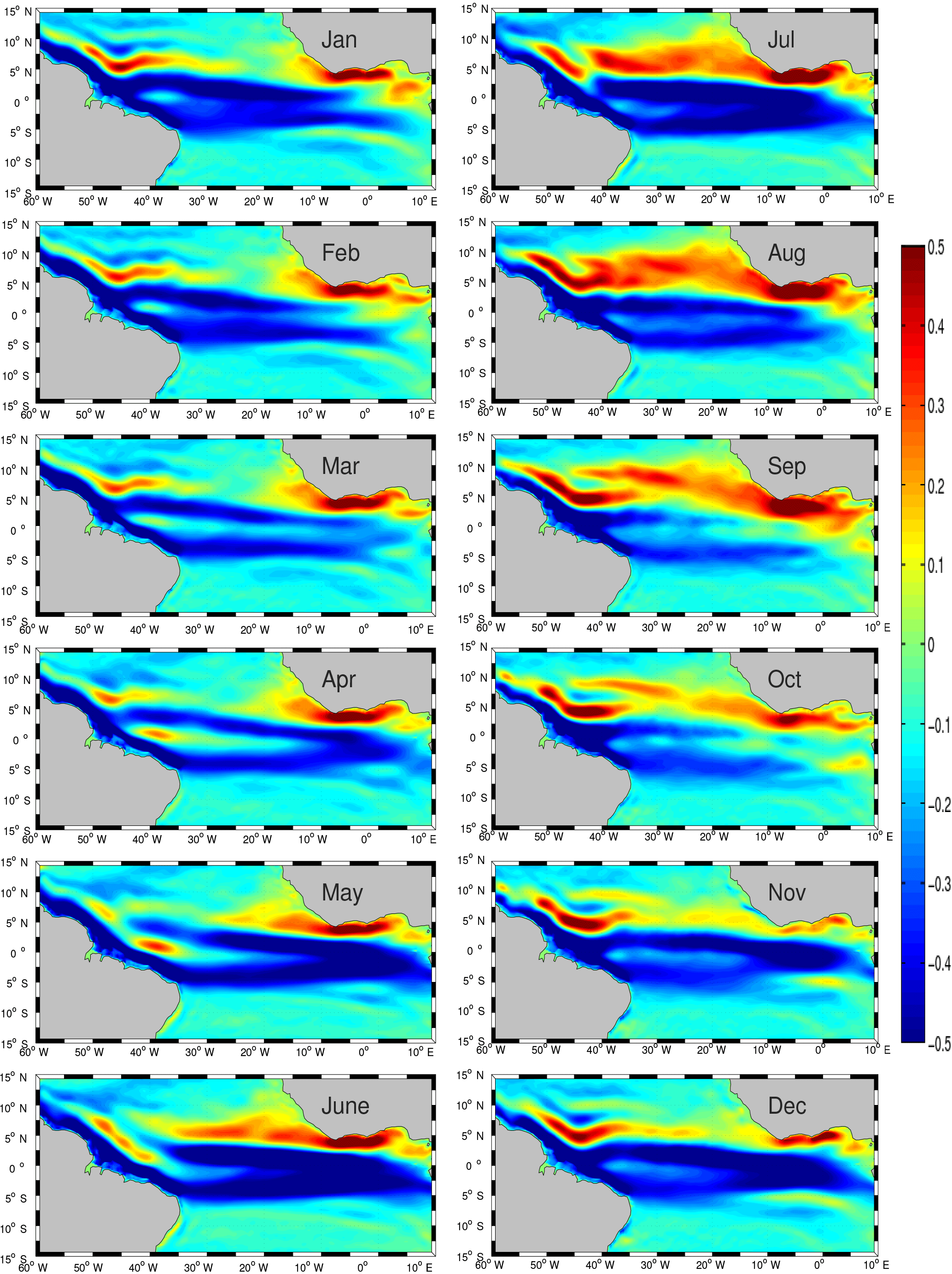
Figure 2Model monthly climatology of zonal velocity at the ocean surface (m s−1). This figure should be compared with Fig. 6 in Rosell-Fieschi et al. (2015).
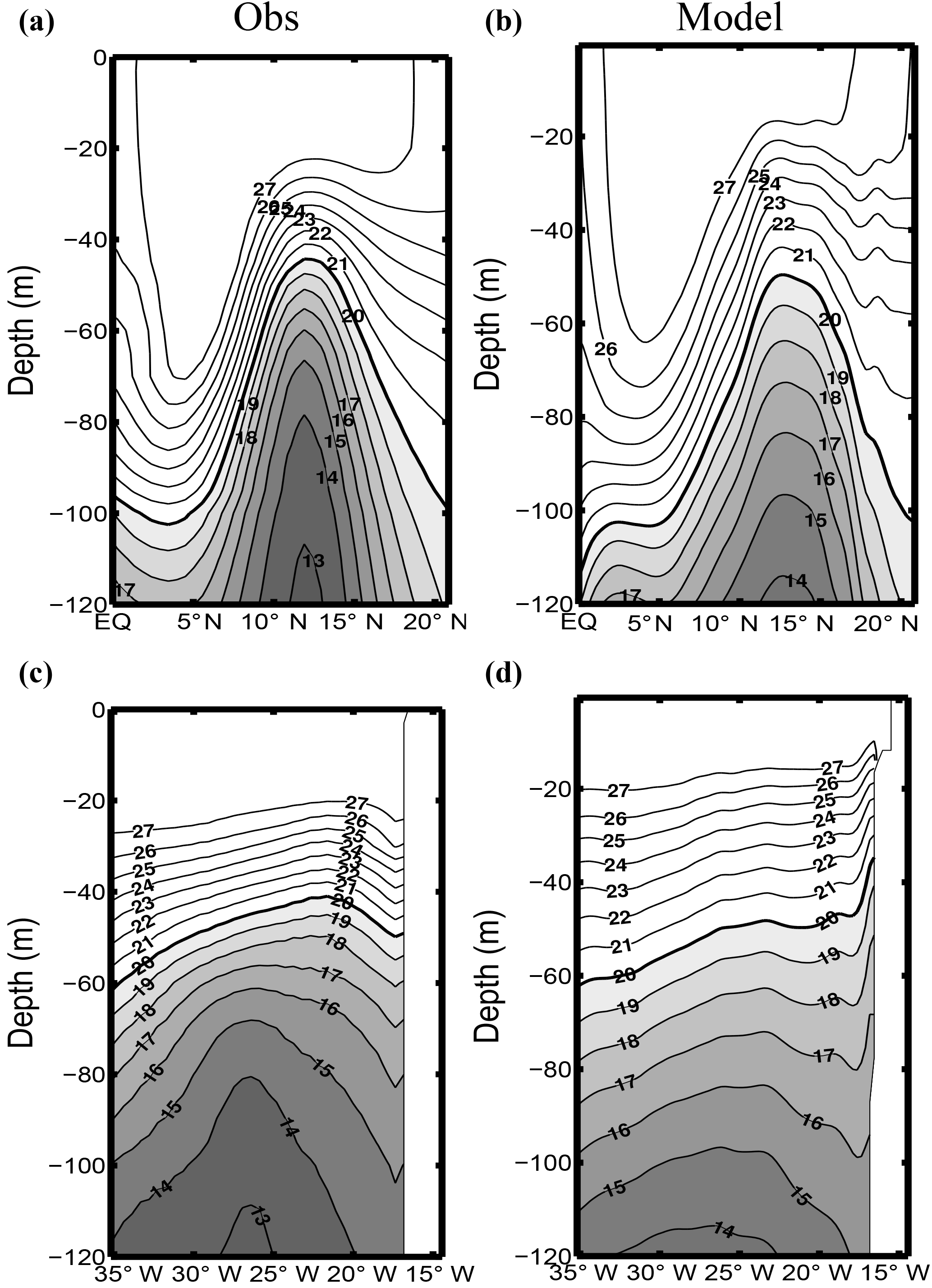
Figure 3Meridional (zonal) section at 26∘ W (a, b) (13∘ N; c, d) for temperature (∘C) averaged during September–October. Observations and models respectively correspond to panels (a, c) and (b, d).
The ETNA broadly coincides with the shadow zone of the North Atlantic subtropical gyre. In classical wind-driven circulation theories it is a place of weak circulation, owing to the no-flow condition at the eastern boundary (Luyten et al., 1983). This means that thermocline waters, including those in our density class of interest, are not directly ventilated even though they outcrop overwhelmingly north of 20∘ N in the negative WSC region (Malanotte-Rizzoli et al., 2000). Strictly speaking though, the ETNA is not part of the subtropical gyre. As mentioned above, it is characterized by regional positive WSC, positive Ekman pumping, and, in virtue of the Sverdrup relation, northward flow (the vertical distribution of which is not well known and will be an important aspect of the present work). Two main dynamical features have been identified in the region that are consistent with these expectations: the Guinea thermal dome and the Mauritanian current.
The Guinea dome has been described in numerous studies (Siedler et al., 1992; Stramma et al., 2005) as a permanent quasi-stationary feature on the eastern side of a quasi-zonal thermal ridge present over most of the basin at ∼12–14∘ N. The dome is characterized by a rise of isotherms in the depth range 50–300 m. Voituriez and Herbland (1982) relate the Guinea dome to the cyclonic rotation of the NECC when approaching the eastern end of the basin, from eastward to northward and then westward as the flow connects to the NEC. Their claim is that the quasi-zonal thermal ridge associated with the NECC is reinforced by this cyclonic rotation, thereby giving rise to the dome structure. Note, though, that the thermal ridge is much more visible (in meridional cross sections; Fig. 3a, b) than the thermal dome (in zonal cross sections; Fig. 3c, d). Despite its supposed importance in conveying waters rich in dissolved oxygen toward the North Atlantic OMZ (Peña-Izquierdo et al., 2015), the Guinea dome remains to this date an elusive circulation feature, with limited and contradictory results on its position, dynamics, and variability, as this overview of the literature indicates. Siedler et al. (1992) analyze the Guinea dome structure and seasonal variability using in situ observations and a primitive equation model. Based on temperature distribution and geopotential anomaly fields, they conclude that the Guinea dome is a permanent feature with some seasonal variability, the upper thermocline center of the dome being found at about 9∘ N, 25∘ W in summer and 10.5∘ N, 22∘ W in winter. Their conclusions partly contradict earlier studies that could not identify the upper thermocline expression of the dome in winter (Voituriez, 1981) and the issue has not been settled since then (Lázaro et al., 2005). Finally, note that ADCP measurements (Stramma and Schott, 1999; Stramma et al., 2005, 2008) or averaged float drifts (Stramma et al., 2008) show weak signs of westward flow on the northern side of the Guinea dome in contrast to many schematic representations of the circulation associated with the Guinea dome (Brandt et al., 2010; Stramma and Schott, 1999; Stramma et al., 2005).
Modeling has not led to much clarification, perhaps because the Guinea dome is seldom reproduced with fidelity. The doming of the isopycnals along zonal sections is clearly insufficient in the models of Siedler et al. (1992), Yamagata and Iizuka (1995), Stramma et al. (2005), and in ours (see below). In contrast, OFES simulations presented by Doi et al. (2009) tend to overestimate the doming (see their Fig. 2c and d). More problematically, these simulations exhibit ETNA thermohaline uplifts that have distinct characteristics compared to the real Guinea dome. For instance, in Yamagata and Iizuka (1995) the subsurface temperature field exhibits a cold coastal tongue between 10 and 25∘ N that protrudes offshore around 15∘ N (their Fig. 3). The cold tongue is quasi-stationary, while the protrusion is subjected to an important seasonal modulation. Neither the model cold tongue nor the protrusion can unambiguously be identified to match the observed Guinea dome structure.
In terms of dynamical interpretation, the Guinea dome is being systematically related to WSC forcing, but two variant explanations can be found in the literature: local forcing (Mittelstaedt, 1976; Yamagata and Iizuka, 1995) or large-scale forcing with some Rossby wave effects (Siedler et al., 1992). Historically, this disagreement has flourished in a context of large uncertainties on the WSC patterns (Townsend et al., 2000). The QuikSCAT climatology now allows us to unambiguously demonstrate that the Guinea dome position does not coincide with that of a WSC extremum so the dynamical rationalization for the existence and position of the dome remains to be improved. In Part 2 the Guinea dome will be considered in the regional circulation context. Herein we focus on the flow over the WA continental slope (also referred to as coastal flow given the regional perspective of this work) in the ETNA region, i.e., between approximately 8 and 20∘ N.
In this latitude range, the existence of upper ocean poleward currents over the WA continental slope has been reported for a long time but only the basic aspects of their structure (vertical and horizontal) and seasonal variability are known. Two seasons of intensified poleward flow can be inferred from the literature (Barton, 1989; Wooster et al., 1976). During the upwelling season (winter–spring), a poleward undercurrent naturally develops as also found in the other upwelling systems (Barton, 1998; Hughes and Barton, 1974). In summer–fall another poleward flow intensification occurs (Mittelstaedt, 1991). In contrast to the earlier one, the flow is surface intensified and the surface part of the flow is sometimes referred to as the “Mauritanian current” following Kirichek (1971). This characteristic and an approximate coincidence in time has led to the suggestion that this poleward flow pulse results from the bifurcation of the summertime northern branch of the NECC as it approaches WA (Kirichek, 1971; Lázaro et al., 2005; Mittelstaedt, 1991). But the specifics of the flow bifurcation (from zonal to meridional) have, to our knowledge, never been described in dynamical terms. Alternatively or complementarily, some authors invoke upwelling wind relaxation south of ∼21∘ N (Mittelstaedt, 1991) as the driving process for the summer–fall pulse of poleward flow. Older studies tend to insist on an origin in the Gulf of Guinea for the summer pulse (Kirichek, 1971; Mittelstaedt et al., 1975) but this process has not been revisited for a long time. In his 1989 review study Barton qualifies the knowledge of the poleward undercurrent along the eastern boundary of the North Atlantic as sketchy: “the arguments for its existence as a continuous entity are based upon relatively few direct current observations, some interpretations of temperature and salinity data, and a degree of speculation”. Almost 30 years later, the situation is virtually unchanged with only a few irregular ship ADCP transects to describe the boundary current system (Peña-Izquierdo et al., 2012; Schafstall et al., 2010). In particular, the works of Kirichek (1971), Mittelstaedt (1972), Hughes and Barton (1974), and a few follow-up (Tomczak, 1989) and review studies remain the main sources of observational knowledge about the WA slope currents between 10 and 20∘ N (between 5 and 10∘ N observations are even fewer).
In this context the point raised by Barton (1989) about whether the poleward undercurrent and the more seasonally intermittent surface countercurrent (also called the Mauritanian current) are dynamically distinct entities is still pending. The use of two different names to describe the poleward flow depending on depth range implicitly suggests they are dynamically distinct. We instead will prefer to use the unique and neutral terminology “WA poleward boundary current” (or WABC in short) to refer to the northward flow present over or in the vicinity of the WA continental slope.
This overview strongly suggests that clarifications are needed on ETNA circulation and dynamics. The present study and a companion paper (Part 2) are a contribution to this needed effort. The focus is on waters within the density class that most strongly responds to wind forcing because they are transported by the Sverdrup flow and/or actively contribute to upwelling in the ETNA sector, driven by Ekman pumping or coastal divergence. Due to the sparseness of observations in this region modeling can be an invaluable source of information. Our approach will essentially be based on the careful analysis of an eddy-permitting NEMO model simulation (Madec, 2014). In this Part 1, the realism of the modeled circulation and thermohaline structure is evaluated in Sect. 3 and will be deemed sufficient to inform several related aspects of the WA ocean dynamics. The seasonal cycle of the WABC will then be presented (Sect. 4). Its underlying dynamics will subsequently be explored and discussed over the continental slope in relation to wind-forced coastal trapped wave theory (Sect. 5) and offshore in relation to Rossby wave theory (Sect. 6). In light of these results and interpretations, a general assessment of the knowledge, knowledge gaps, and model biases pertaining to the WA boundary current will be proposed (Sect. 7). The source pathways for WA coastal upwelling waters and the broader regional circulation (which turns out to be of key relevance to understanding these pathways) will be examined in Part 2.
In this study, we use a numerical model, the oceanic component of the Nucleus for European Modelling of the Ocean program (Madec, 2014). It solves the three-dimensional primitive equations discretized on an Arakawa C grid at fixed vertical levels (z coordinate). The grid horizontal resolution is 1∕4∘ and the configuration (referred to as TROP025 hereafter) generously covers the tropical Atlantic (35∘ S–35∘ N, 100∘ W–15∘ E). TROP025 has 75 vertical levels, 12 (24) being concentrated in the upper 20 m (100 m). It is forced at its lateral boundaries with daily outputs from the MERCATOR global reanalysis GLORYS2V3 (Masina et al., 2015). The open boundary conditions radiate perturbations out of the domain and relax the model variables to 1-day averages of the global experiment. Details on the numerical methods are given in Madec (2014). At the surface, the atmospheric fluxes of momentum, heat, and freshwater are provided by bulk formulae (Large and Yeager, 2004). The simulation is forced with the Drakkar Forcing Set DFS5.2 (Dussin et al., 2014), which is mainly based on the ERA-Interim reanalysis (Dee et al., 2011). DFS5.2 consists of 3-hourly fields for wind speed, atmospheric temperature, and humidity and daily fields for longwave radiation, shortwave radiation, and precipitation.
Some model–data comparisons are available in Da-Allada et al. (2017) and Jouanno et al. (2017). Additional evaluation directly related to this study is presented in the next section. It largely relies on the gridded version of the Coriolis dataset for reanalysis version 4.2 (hereafter CORA4.2, http://www.seanoe.org/data/00351/46219/, last access: 18 August 2018) for potential temperature and salinity over the period 1990–2014. Its resolution is but the gridding software ISAS (Gaillard et al., 2016) involves correlation length scales that far exceed this mesh grid size, which is detrimental to the representation of boundary currents such as the one we are interested in. CORA4.2 includes the vast majority of available ARGO profiles and offers a state-of-the-art description of the recent oceanic thermohaline state. The model solution corresponds to a longer period (1979–2015) but this is deemed inconsequential given the limited regional low-frequency variability. In addition, note that a 15–20 % fraction of the CORA bins within 1000 km from the WA shore have their monthly climatology built with less than 20 T–S vertical profiles (not shown). There are thus substantial uncertainties in the true ETNA climatological state irrespective of the period. For more information on CORA4.2 readers are referred to Cabanes et al. (2013).
Mathematical symbols have their usual meaning. T, S, σt, and ρ respectively refer to potential temperature, salinity, potential density anomaly, and in situ density. The variables x (y) and u (v) refer to zonal (meridional) directions and velocity. At any (x, y) position, we define the depth anomaly for a specific isotherm T0 as the depth of that isotherm minus that of its long-term climatological mean.
Many diagnostics involve vertical integration between the surface and the isopycnal surface σt=26.7 kg m−3. U26.7 and V26.7 are vertically integrated zonal and meridional transports over that depth range. The geostrophic part of the transport is noted with a “g” subscript. At this stage the choice of 26.7 may seem arbitrary but it will be justified by several model analyses below and in Part 2. In particular, it will be shown that the layer above σt= 26.7 includes an overwhelming fraction of the Sverdrup and upwelling circulation in the model. σt=26.7 is also convenient because subsurface waters lighter than this value are overwhelmingly of the SACW type, in contrast to deeper waters (Peña-Izquierdo et al., 2012, 2015).
For reference, the geostrophic part of the Sverdrup volume transport denoted Vsv is defined as (Cushman-Roisin and Beckers, 2011)
where f is the Coriolis parameter, its derivative with respect to the meridional coordinate, ρ0 is a reference density equal to 1025 kg m−3, and (τx, τy) is the surface wind stress (in N m−2).
Dynamic heights are presented in Sect. 3. They are calculated at 50 dbar relative to 500 dbar according to the standard formula (Talley, 2011)
with the additional assumption that pressure and depth are equivalent. The associated geostrophic flow is classically given by
Potential vorticity (PV) is examined in the context of Rossby wave dynamics in Sect. 6. It is expressed in density coordinates for a fluid layer of thickness h between the potential density surfaces σ1 and σ2 (Cushman-Roisin and Beckers, 2011):
where ξ is the vertical component of relative vorticity for the flow in this fluid layer, which can be neglected given the smallness of the Rossby number associated with the eastern boundary conditions under consideration.
In several instances, we wish to rotate the flow or wind at the model shelf break to isolate their alongshore and/or along-slope component. To do so velocities are rotated with respect to the orientation of the shelf break. This orientation is computed at every grid point following the 100 m isobath using centered differences. A total of 15 passes of a three-point filter with coefficients (0.25, 0.5, 0.25) are subsequently applied to ensure some smoothness to the angle used for the along-slope projection.
In this section we carefully evaluate our simulation with respect to available observations, mainly from the CORA4.2 database. As mentioned in the previous section, time periods for the model and observations do not match precisely. In addition observations are not particularly dense in our region of interest (although many of the bins have ∼100 measurements per climatological month) so we are concerned with a qualitative assessment of model realism.
We start by comparing the monthly climatology of surface zonal currents in TROP025 with the climatology derived from ARGO drifts obtained by Rosell-Fieschi et al. (2015). The agreement is quite remarkable both in terms of spatiotemporal patterns and current magnitude (compare Fig. 2 with their Fig. 6). The model captures the northern and equatorial branch of the South Equatorial Current whose separation is most clear in boreal spring, as also found in the observations. More importantly for our study, the NECC seasonal cycle is realistic both in terms of north–south displacement (northernmost extension and widest latitude range in August–September) and change in flow magnitude (swiftest currents >0.3 m s−1 found in July–August). Note though that peak NECC currents in TROP025 seem a bit weaker than observed. The eastward-flowing Guinea current, whose seasonal variability will turn out to be of relevance for the WABC, is also adequately represented. It is intensified between 10 and 0∘ W with a slight peak in boreal summer and a marked decrease in flow speed from September (when the Guinea current is strongest) to November. North of 10∘ N within 5–10∘ from the West African coast observed zonal velocities are weak and variable but generally oriented westward. This westward tendency is less marked for model velocities. This discrepancy may at least partly be related to Stokes drift, which is mainly zonal, can reach about 0.05 m s−1 in that region, and affects surfacing ARGO floats (Rosell-Fieschi et al., 2015).
Outside the equatorial region where TROP025 behaves adequately (Da-Allada et al., 2017) we cannot more precisely evaluate the model circulation from direct observations but the equatorial and tropical Atlantic thermohaline structure is overall quite well represented. This is evident from a model–data comparison of climatological temperature along two vertical sections (Fig. 3) at 13∘ N and 26∘ W. The latter crosses the thermal ridge associated with the NECC. The position of the zonal section is chosen at the latitude typically associated with the Guinea dome. Following Siedler et al. (1992) and Doi et al. (2009) these fields are shown for the September–October period during which the Guinea dome is supposed to be most marked, but model–data agreement and differences are quite similar for other months. Along 26∘ W thermocline displacements with latitude are quite faithfully reproduced. For example, the deepening of the 20 ∘C isotherm from 12∘ N at the top of the thermal ridge to 20∘ N is ∼55 m in the observations vs. 50 m in TROP025. The main bias concerns the sharpness of the thermocline, which is insufficient, presumably as a consequence of an overly strong model diapycnal diffusivity. As a consequence, temperature is 1.5 ∘C too high at 100 m of depth in the vicinity of the thermal ridge. A similar bias is found along 13∘ N where the model thermocline is too diffuse. Along that section, the dome structure is manifest in the model with a deepening of the isotherms colder than ∼20 ∘C toward the coast, albeit with less amplitude than found in the observations. As in the observations the longitude east of which the deepening occurs shifts westward for colder isotherms. On the other hand, TROP025 is unable to produce the limited vertical displacement observed east of 20∘ W for isotherms above 20∘. So overall, the modeled Guinea dome present in TROP025 is weaker than observed. This model bias is common (Siedler et al., 1992; Yamagata and Iizuka, 1995), with the notable exception of Doi et al. (2009). We suspect that this bias is also reflected in the intensity of poleward velocities that may be underestimated in TROP025.

Figure 4Summer (June–September, a, b) and winter (December–February, c, d) mean dynamic height at 50 m relative to 500 m (m2 s−2). The contour interval is 1 m2 s−2. The associated geostrophic circulation is also shown (vectors). Panels (a, c) are for observations (TROP025). To ease comparison with the observations, 3 m2 s−2 was uniformly subtracted from the model fields.
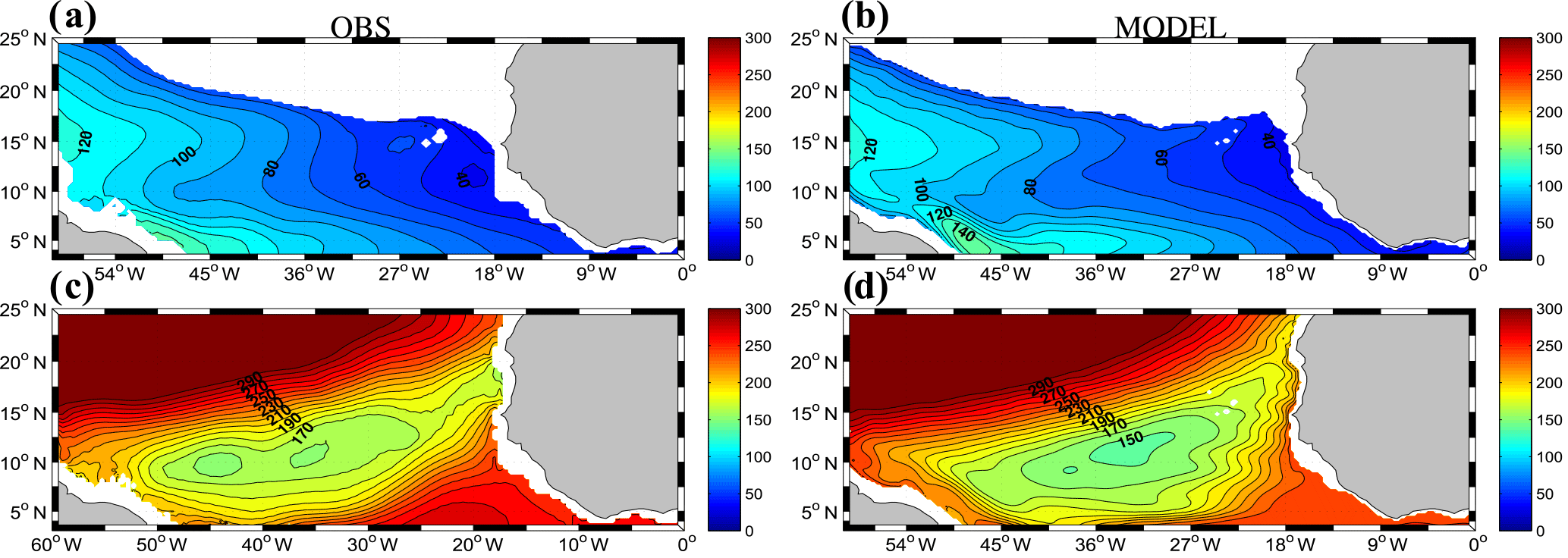
Figure 5Depth (m) of the isopycnal density surface σt=25.2 (a, b) and σt=26.7 (c, d) in CORA (a, c) and TROP025 (b, d).
Seasonal climatologies of dynamic height ΔD50∕500 (see mathematical definition in Sect. 2) shown in Fig. 4 for winter and summer confirm this suspicion. Model and observation general patterns are consistent with each other on the NEC and NECC signatures and their winter–summer changes. The position and intensity of the NECC is quite similar over most of the domain for both seasons, particularly in summer. In winter, the precise form of the cyclonic circulation around the Guinea dome is less well reproduced by the model. The main differences are east of 24∘ W where the model NECC exhibits some meanders not seen in the observations. A northward branch is evident in the model and observations but the model flow turns more gradually, starting from further to the west at ∼25∘ W than in the observations (e.g., compare geopotential lines 63 in summer). East of 20∘ W the tilt of the geopotential lines is noticeably different in the model and the observations. The regional-scale meridional gradient of geopotential in the ETNA is significantly stronger in the observations than in TROP025, respectively 7 vs. 4 m2 s−2 in summer and 6 vs. 2.5 m2 s−2 in winter. Implications of this bias will be discussed in Part 2, but we note again that model regional circulation is in good qualitative agreement with observations.
Our analyses will systematically use the isopycnal surfaces σt=26.7 and, more infrequently, σt=25.2 because they approximately limit the range of subsurface waters involved in the model WA coastal upwellings and meridional transport. In Fig. 5 we show the climatological depth of these two isopycnal surfaces in the model and CORA observations. Qualitative agreement between the two is evident, e.g., in terms of outcrop line position, east to west deepening tendency for σt=25.2, and shape and amplitude of the σt=26.7 doming in the central part of the basin. Very close to shore along WA the model σt=26.7 isopycnal surface is not close enough to the surface, presumably because our eddy-permitting resolution is insufficient to adequately resolve the coastal upwelling per se (Capet et al., 2008). However, this bias is limited to ∼20 m and is not crucial for the present continental slope and open ocean investigation.
In attempting to explain the WABC seasonal cycle we will focus on the dynamics along the coast of the Gulf of Guinea. Therefore, a model evaluation is conducted at 4∘ N, 5∘ W, i.e., over the continental slope south of Abidjan, Ivory Coast. The seasonal cycle of temperature T(z) at this location was reported by Picaut (1983) for the period 1957–1964 (see his Fig. 15b). Comparison with our Fig. 6 reveals the good level of realism of TROP025. Most noticeably, the model produces a semiannual oscillation of the thermocline that is most pronounced in the depth range 50–150 m with the highest (lowest) temperatures reached in April and October–November (August and January). Model oscillations resemble the observations in terms of phase, upward propagation of the summer–fall doming tendency, and contrast in amplitude between the winter–spring (weak) and summer–fall (strong) oscillations. On the other hand, a quantitative difference concerns the amplitude of the oscillations, which are underestimated by 50 % or more in the model, e.g., 30 m (50 m) peak to peak amplitude for the seasonal cycle of δz16 in TROP025 (in the observations). This bias is particularly pronounced below 150 m. Finally, we note that the marked deepening phase between July and October is better captured than the preceding shallowing phase. The latter occurs more rapidly in the observations, e.g., over a 2-month period in June–July for the 16 ∘C isotherm vs. 3–4 months in the model. To put these biases into perspective it would be useful to know the degree to which the very local conditions at 4∘ N, 5∘ W that TROP025 does not represent (e.g., fine-scale irregularities of the shoreline or continental shelf–slope bathymetry) contribute to the observed seasonal cycle.
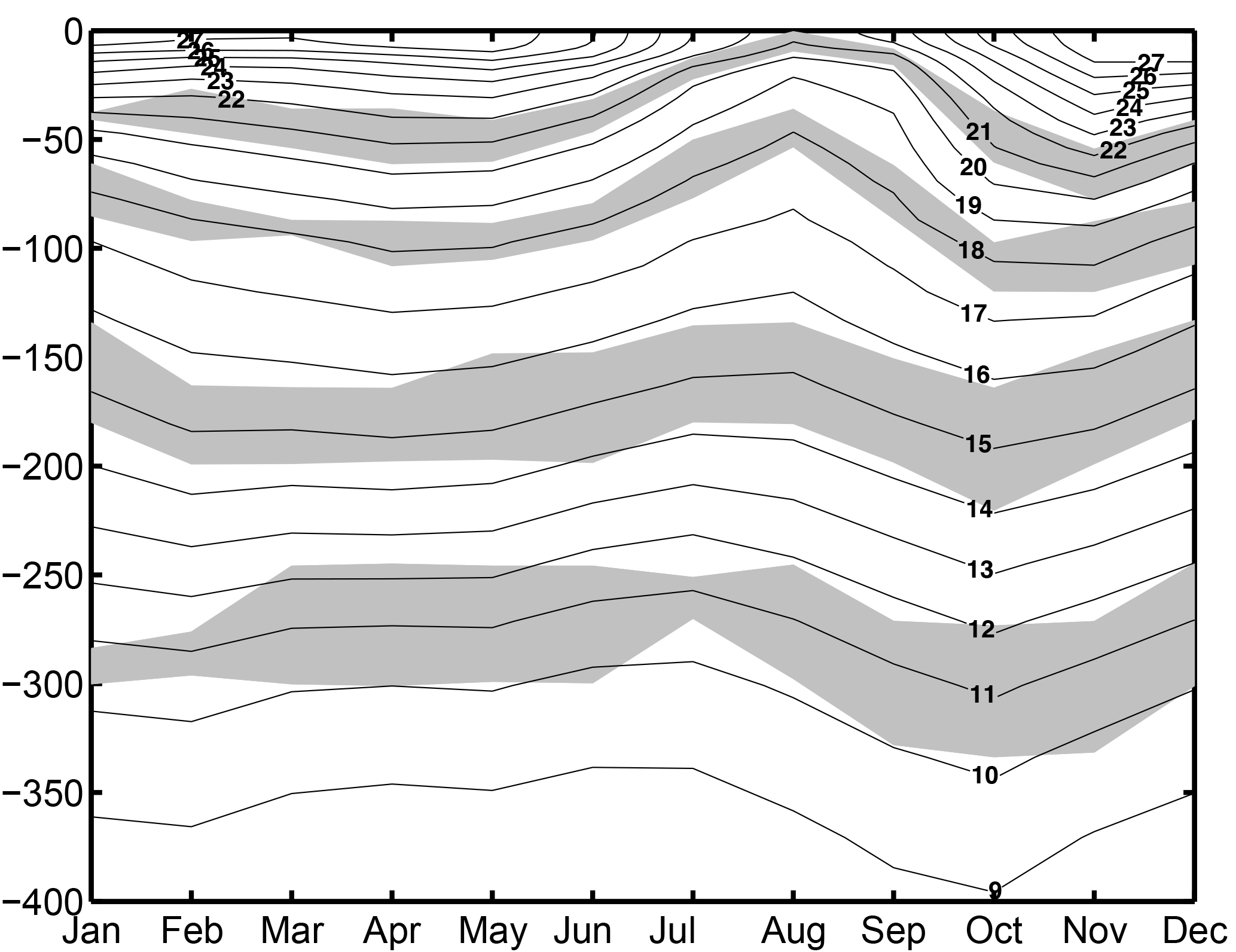
Figure 6Time–depth representation of TROP025 climatological temperature (∘C) at 4∘ N–5∘ W over the period 1982–2012. This figure should be compared with the climatological cycle observed at the same location between 1957 and 1964 (Picaut, 1983). To evaluate uncertainty 24 model climatologies were computed using 8-year averaging periods as in the observations (with starting years from 1982 to 2005); the shallowest and deepest positions of four isotherms (11, 15, 18, and 21 ∘C) over this ensemble are shown with gray shading and indicate the limited role played by interannual variability, particularly for the 18 and 21 ∘C isotherms.
Overall, the model climatological traits and dominant patterns of seasonal variability are quite realistic, both at basin scale and more locally in the ETNA. Our conclusion is thus that the model circulation and thermohaline structure possesses a sufficient degree of realism to warrant further in-depth analysis. In our discussion of the real ETNA dynamics and circulation (Sect. 7 and likewise in Part 2) we will keep in mind the biases that have also been identified, including the relative weakness of the model poleward flow along WA.
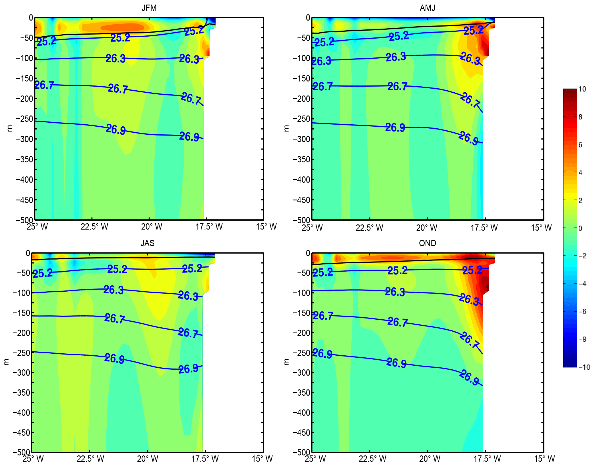
Figure 7Seasonally averaged vertical–zonal section of meridional velocity (in colors; cm s−1), σt (blue lines; kg m−3), and mixed layer depth (black line; in meters) averaged between 13 and 15∘ N.
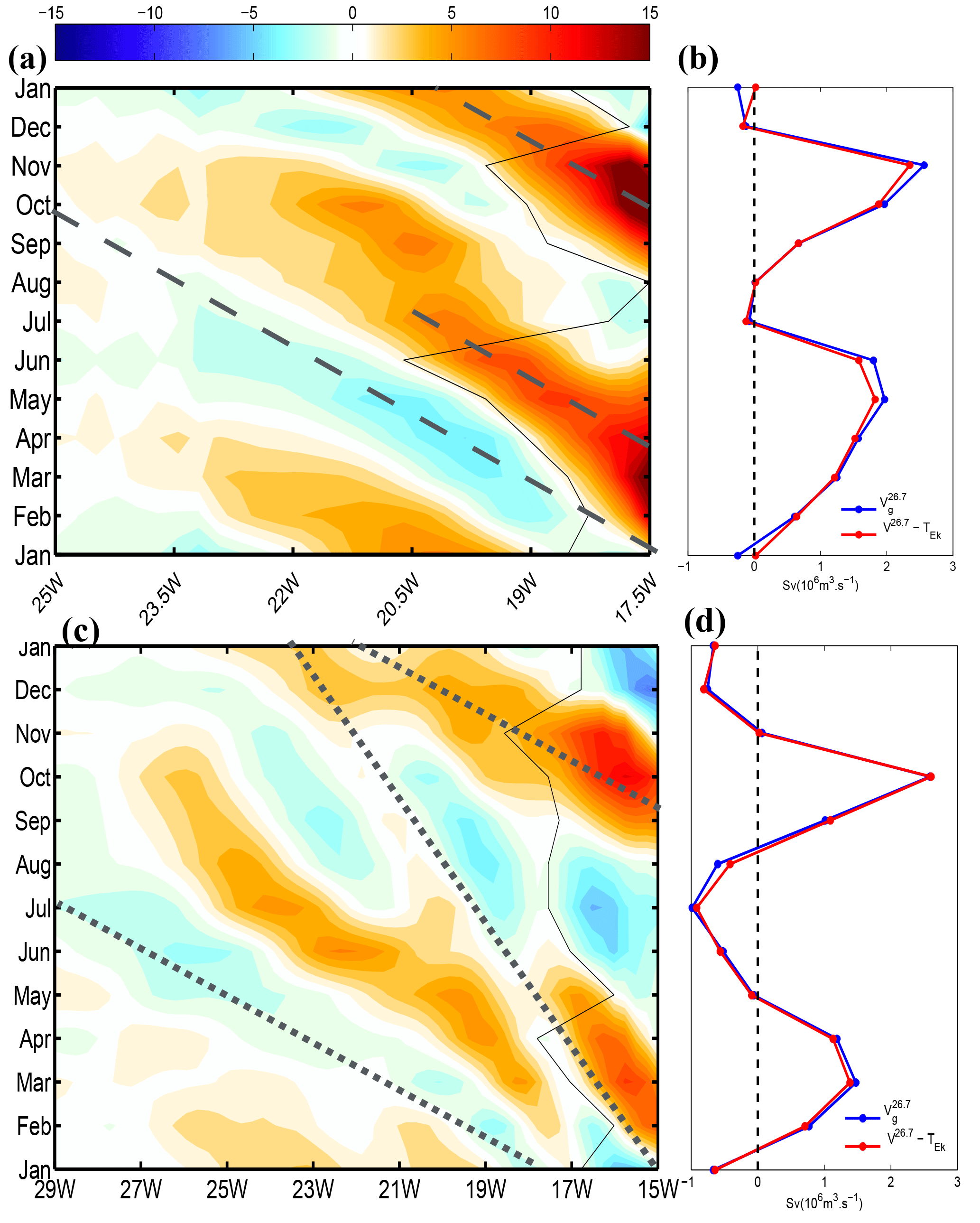
Figure 8(a, c) Time–longitude diagram of vertically integrated meridional transport (m2 s−1) averaged along-slope between 13 and 15∘ N (a) and between 7 and 9∘ N (c). Propagation speed at 3.5 cm s−1 (a) as well as 7.4 and 3 cm s−1 (c) is shown with dashed lines. These values are the ones we choose as most appropriate to describe the propagation of patterns in the diagrams. (b, d) Associated climatologies of meridional transport integrated vertically and across-shore. Vertical integration is performed from the isopycnal surface σθ=26.7 up to the bottom of the mixed layer (a, c and red curve in b, d) or up to the surface but excluding Ekman transport; i.e., we only take into account the geostrophic flow (blue curve in b, d). Across-shore integration is performed from the shoreline to the first location where vertically integrated transport vanishes with a maximum longitude range of 3∘ (integration limit is indicated with the thin solid line in a and c).
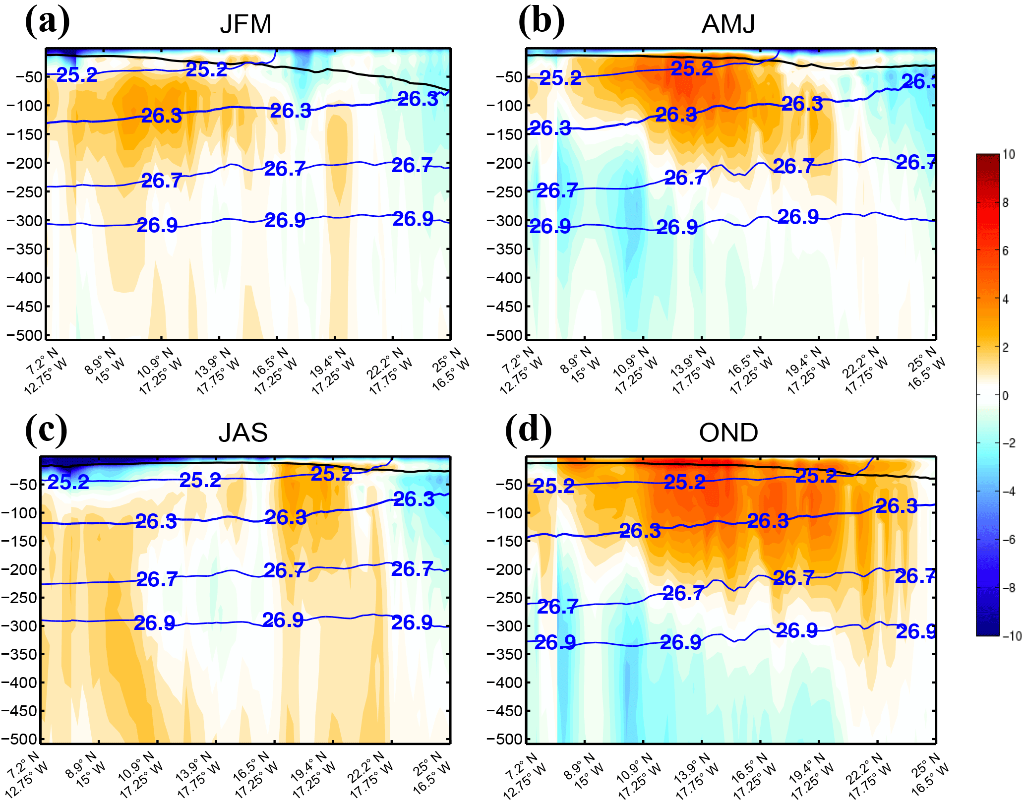
Figure 9Seasonally averaged vertical section of along-slope velocity (in colors; cm s−1), σt (blue lines; kg m−3), and mixed layer depth (black line; in meters) following the shelf break (across-shore averaging between the 100 m isobath and six grid points 150 km offshore).

Figure 10Monthly climatology of meridional transport (m2 s−1) integrated between the isopycnal surfaces σt=26.7 and the surface, excluding wind-driven Ekman transport calculated from TROP025 wind fields. The two thin dashed lines represent the location where zero PV gradients are found in Fig. 17.
Poleward boundary currents are ubiquitous along eastern boundary continental slopes (Brink et al., 1983; Connolly et al., 2014; Huyer, 1983), particularly those subjected to upwelling-favorable winds for which subsurface undercurrents are essential flow features (McCreary, 1981; McCreary et al., 1987; Philander and Yoon, 1982). WA is no exception (Barton, 1989). Poleward currents are present in TROP025 as revealed by the seasonally averaged zonal transects of v (Fig. 7). Figures 8–10 offer complementary views of the structure and seasonality of the WABC.
At 14∘ N (i.e., at a central location in the ETNA) a poleward undercurrent is visible over the continental slope for all seasons except in summer (July–September) but it is most marked in fall and to a lesser extent in spring (Fig. 7; hereafter we refer to these two poleward flow intensification periods as Pf and Ps, respectively). The undercurrent appears to be strongly baroclinic with deviations of the isopycnals changing sign in the vertical: upward toward the shore above ≈75 m of depth and downward below. Isopycnal displacements reach ∼100 m for the 26.7 isopycnal between 25 and 17.5∘ W. The core of the undercurrent is located at 50 to 100 m of depth with peak velocities reaching 6–8 cm s−1. In fall surface currents are oriented poleward. The absolute flow maximum is found at ∼18∘ W and coincides with the mixed layer base. This surface-intensified flow is the model “Mauritanian current”. A near-surface secondary maximum is also present in spring at approximately the same longitude and depth. In winter and summer a core of weak poleward flow present a few hundred kilometers from shore is suggestive of the radiation of westward-propagating Rossby waves from the continental slope as also found in other regions (Colas et al., 2008; Ramos et al., 2006; Rao et al., 2010; Vega et al., 2003), particularly in the tropics. This is confirmed with a time–longitude diagram of vertically integrated meridional geostrophic transport at about 14∘ N (integration bounds for the integral follow the isopycnal surface σt=26.7 and surface; see Sect. 2). The former broadly coincides with the bottom of the poleward flow. The diagram (Fig. 8a) exhibits clear signs of westward propagation with a speed around 3.5 cm s−1 and a dominant wavelength of about 650 km. The signal amplitude decreases dramatically over 3–5∘ of longitude. Similar or even shorter scales of attenuation are obtained for other semiannual Rossby signals emanating from eastern boundary systems (Dewitte et al., 2008; Gómez-Valdivia et al., 2017).
At 8∘ N (i.e., the southern end of our study region), the time–longitude variability of the meridional transport is more complex. Two propagation speeds can be identified (Fig. 8c) but the patterns are not those expected from a simple superposition of two waves. The processes at stake in the generation of the ETNA Rossby wave field and the possible reasons underlying their rapid offshore attenuation at 14∘ N are discussed in Sect. 6.
As a future point of comparison to other transport estimates, we compute the meridional transport vertically and zonally integrated at 8 and 14∘ N. Zonal integration is performed from the coast to the first offshore location where the flow changes direction with a maximum longitude range of 3∘, so the width over which this transport is achieved varies in time. At 14∘ N, the flow is poleward all year except for two brief periods of weak equatorward flow in January and July. The poleward transport along the WA boundary is seasonally variable with peak values reaching 2 Sv or more during the two peak seasons in May–June and September–November, with differences between Ps and Pf being around 20 % (2 Sv in spring vs. 2.5 Sv in fall). Compared to 14∘ N, the transport seasonal cycle at 8∘ N is more symmetric around 0 (equatorward flow is marked in summer and late fall to early winter; spring intensification is weaker) with the notable exception that the fall intensification reaches similar values in both latitude ranges.
Along-slope vertical sections of seasonally averaged along-slope current are shown in Fig. 9. For each latitude, the current intensity is obtained by across-slope averaging the along-slope flow between the 100 m isobath and 150 km offshore (six grid points); i.e., Fig. 9 is representative of the flow over the continental slope. The regional-scale coherence of the WABC is clearly visible although some minor flow discontinuities result from meandering and eddy formation in the vicinity of the major capes as better seen in Fig. 10 (Djakouré et al., 2014). The northern bound of the poleward flow varies significantly between Ps and Pf (20∘ N vs. 25∘ N, respectively). The surface flow is stronger during the latter but poleward currents are otherwise found over a relatively similar depth range that deepens poleward, being located above 100 m (250 m) of depth south of 10∘ N (between 10 and 20∘ N). In fall when the poleward flow reaches further north it extends down to 350–400 m north of 20∘ N. Note that for latitudes between 10 and 20∘ N, σt=26.7 corresponds quite accurately with the bottom depth of the WABC, which partly motivated our choice of this isopycnal.
In winter weak but coherent poleward flow is still present over the latitudinal range 7–15∘ N. Equatorward flow is mainly found north of 20–22∘ N in the nCCS (where the Canary Current hugs the coast) and in the subsurface below the WABC during Ps and Pf. This highlights the importance of baroclinic effects in the dynamics of the flow. In winter and summer intense near-surface equatorward flow is found south of ≈10∘ N, but it is confined to within 50 m of the surface.
The spatiotemporal complexity of the WABC behavior is further revealed in Fig. 10, which shows vertically integrated geostrophic flow from the surface down to σt=26.7. We make several important observations. First, the general coherence of the flow in the meridional direction (timing of the poleward flow intensifications and their relaxation) is noticeable as is a general westward propagation tendency. The meridional flow is organized in strips that appear at the coast and move offshore. The strips become increasingly tilted in the northeast–southwest direction as they move offshore, consistent with a faster westward propagation speed closer to the Equator. This is particularly evident in March and October when examining the two “phase lines”1 corresponding to Ps and Pf, separated by a thin band of equatorward flow. Propagation becomes increasingly ambiguous when approaching Cap Blanc at about 20∘ N.
Finally, although this description of the WABC seasonal cycle strongly suggests the importance of its semiannual cycle2, note that a perfect semiannual oscillation would translate into an exact correspondence between the left and right panels in Fig. 10. In contrast, the winter time interval from Pf to Ps appears to be a bit shorter than the summer interval from Ps to Pf (e.g., poleward transport is present nearshore in February but still absent in August). This is confirmed at 14∘ N by inspection of Fig. 8a. Asymmetry between the meridional flow during Ps and Pf is more generally confirmed by Fig. 8b, which reveals a sharper peak of northward transport for the latter period.
In the ETNA, positive WSC input is a priori a fundamental ingredient in the generation of poleward flow both nearshore (Fig. 10; see Capet et al., 2004; Small et al., 2015, for similar effects in other eastern boundary systems) and at larger scale (Sverdrup, 1947). To be more quantitative, we compare the theoretical Sverdrup transport Tsv and geostrophic WABC transport in TROP025 over the continental slope (Table 1). Geostrophic model transports above 500 and 1000 m of depth, as more commonly estimated in past studies (Marchesiello et al., 2003; Small et al., 2015), are also given. Results differ strongly between the southern, central, and northern ETNA. At 14∘ N, all model estimates correspond to over 75 % Tsv with limited changes when increasing the range of integration. In contrast, model transport increases steadily with the range of integration at 20∘ N, reaching 70 % Tsv when integration goes down to 1000 m. At 8∘ N Tsv is significantly weaker (see also Fig. 1). There, the model transport also increases steadily with depth but with values in systematic excess of the Sverdrup transport estimate, reaching twice Tsv when integration goes down to 1000 m.
Table 1Climatological Sverdrup transport Tsv (geostrophic part, see Sect. 2) computed from DFS5.2 winds over across-shore sectors from the shelf break to 150 km offshore for three different latitudes ranges (2∘ wide centered over the latitude reported in the first column). Model geostrophic transports computed over the same areas are indicated as a percentage of Tsv for three different ranges of vertical integration from the surface to σt=26.7 (, third column), 500 m (V500 m, fourth column), or 1000 m (V1000 m, fifth column).
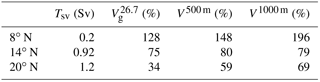
There are several reasons why the percentages in Table 1 are not strict determinations of the fraction of WABC transport that can be attributed to WSC. First, the cross-shore width and transport of the WABC is not uniquely defined because it varies as a function of latitude and time of the year (see our estimation procedure used in Fig. 8b). Bottom pressure torque can also cancel part of the WSC contribution to the barotropic vorticity balance (Molemaker et al., 2015). In addition, momentum fluxes by mesoscale eddies are known to redistribute WSC input, particularly in the across-shore direction (Marchesiello et al., 2003). Most importantly, the Sverdrup balance is a constraint on the total barotropic flow. Thus, although Sverdrup flow tends to be concentrated in the thermocline and above (Anderson and Gill, 1975), the WABC transport as we define it (above σt=26.7) does not solely reflect the Sverdrup balance, but also baroclinic processes and how they vary in time (e.g., on seasonal scales; Fig. 7) and space (e.g., the meridional changes in baroclinic structure; Fig. 9 and Table 1). In this context and pending further progress with model sensitivity experiments we hypothesize that mean poleward transport in the vicinity of the WA continental slope arises from local wind stress curl driving Sverdrup flow plus a combination of baroclinic response to remote wind forcing (McCreary, 1981; Yoon and Philander, 1982) as far as the equatorial band, baroclinic response to meridional gradients of the Coriolis frequency (Hurlburt and Thompson, 1973), and alongshore gradient in wind stress curl (Oey, 1999).
We now turn to the seasonal cycle of the WABC about which more can be said based on the TROP025 experiment alone. The main processes underlying Ps- and Pf-intensified poleward transport could a priori result from four distinct (not mutually exclusive) processes: (i) local generation of a poleward undercurrent in conjunction with variable coastal upwelling conditions, (ii) remote forcing of poleward flow with subsequent propagation in the form of coastal trapped waves, (iii) local modulation of the nearshore Sverdrup transport in relation to the seasonal cycle of the wind stress curl, and (iv) excitation of free Rossby wave modes at the semiannual frequency, e.g., by processes (i)–(iii) if their associated wavenumber–frequency match the dispersion relation.
As mentioned above, large deviations from the Sverdrup balance are possible at fine temporal scale (e.g., sub-annual) (Thomas et al., 2014; Wunsch, 2011), particularly near lateral ocean boundaries (Small et al., 2015). One striking discrepancy between the WABC and corresponding Sverdrup transport concerns their respective seasonal cycles that bear no resemblance, as illustrated in Fig. 11 at 14 and 20∘ N. Over the continental slope at 14∘ N, Sverdrup transport is dominated by an annual cycle that sharply contrasts with the semiannual cycle of (a similar contrast is found for the geostrophic meridional transport computed with integration limits at 500 or 1000 m of depth; not shown). At 20∘ N, the semiannual cycle of the meridional transport is less prominent but differences with the local Sverdrup transport remain important. These arguments lead us to exclude process (iii) as a process responsible for the semiannual cycle of the WABC. In the remainder of this section the respective roles of (i) and (ii) are considered, while the possible role of (iv) will be discussed in the next section.
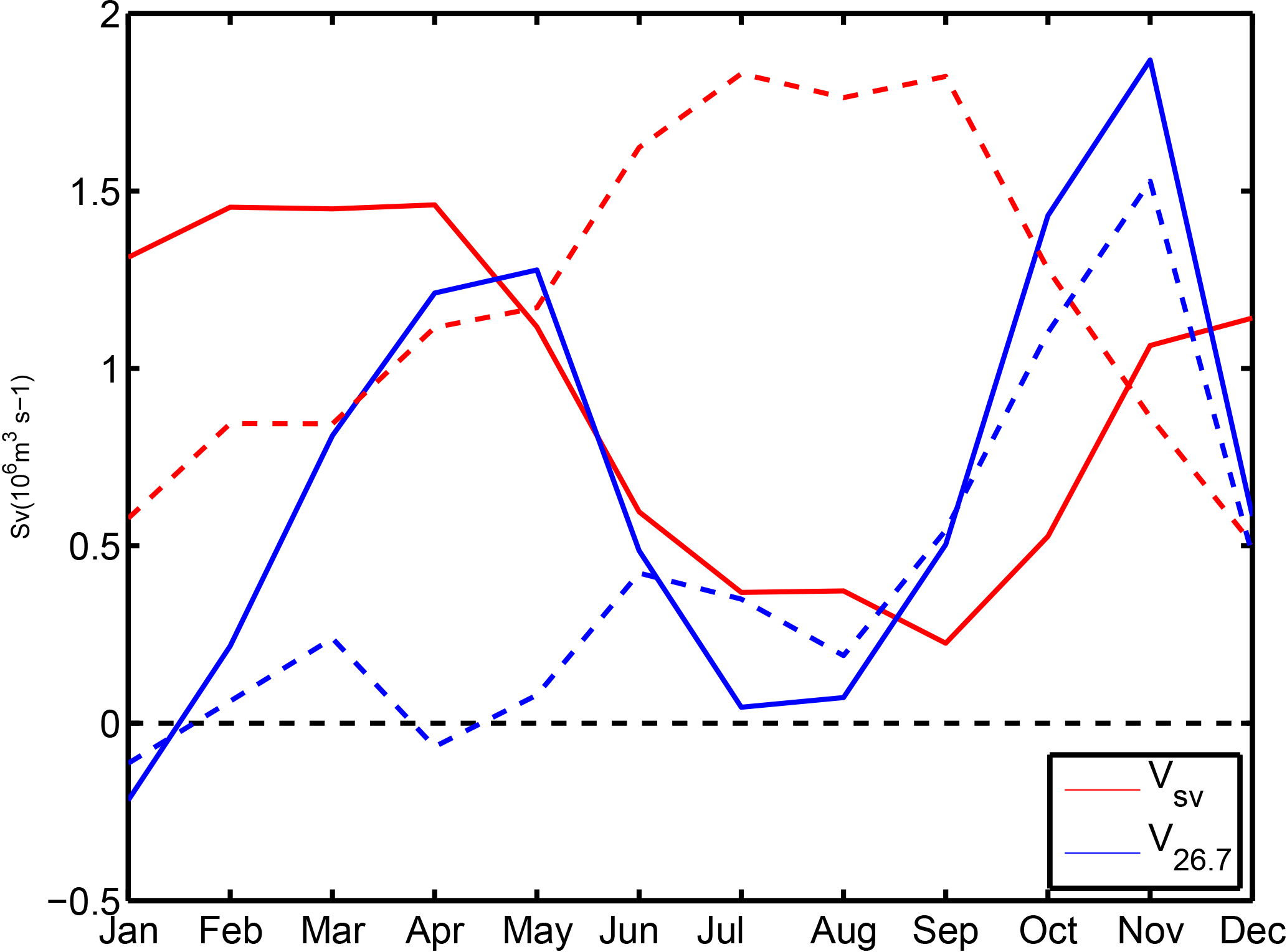
Figure 11Seasonal cycle of Sverdrup transport (red lines) and meridional geostrophic transport vertically integrated between σt=26.7 and the surface (blue lines). Both transports are across-shore integrated between the 100 m isobath and six grid points offshore. Solid lines are for the Cape Verde region (13–15∘ N), while dashed lines are for the Cap Blanc region (19–21∘ N).
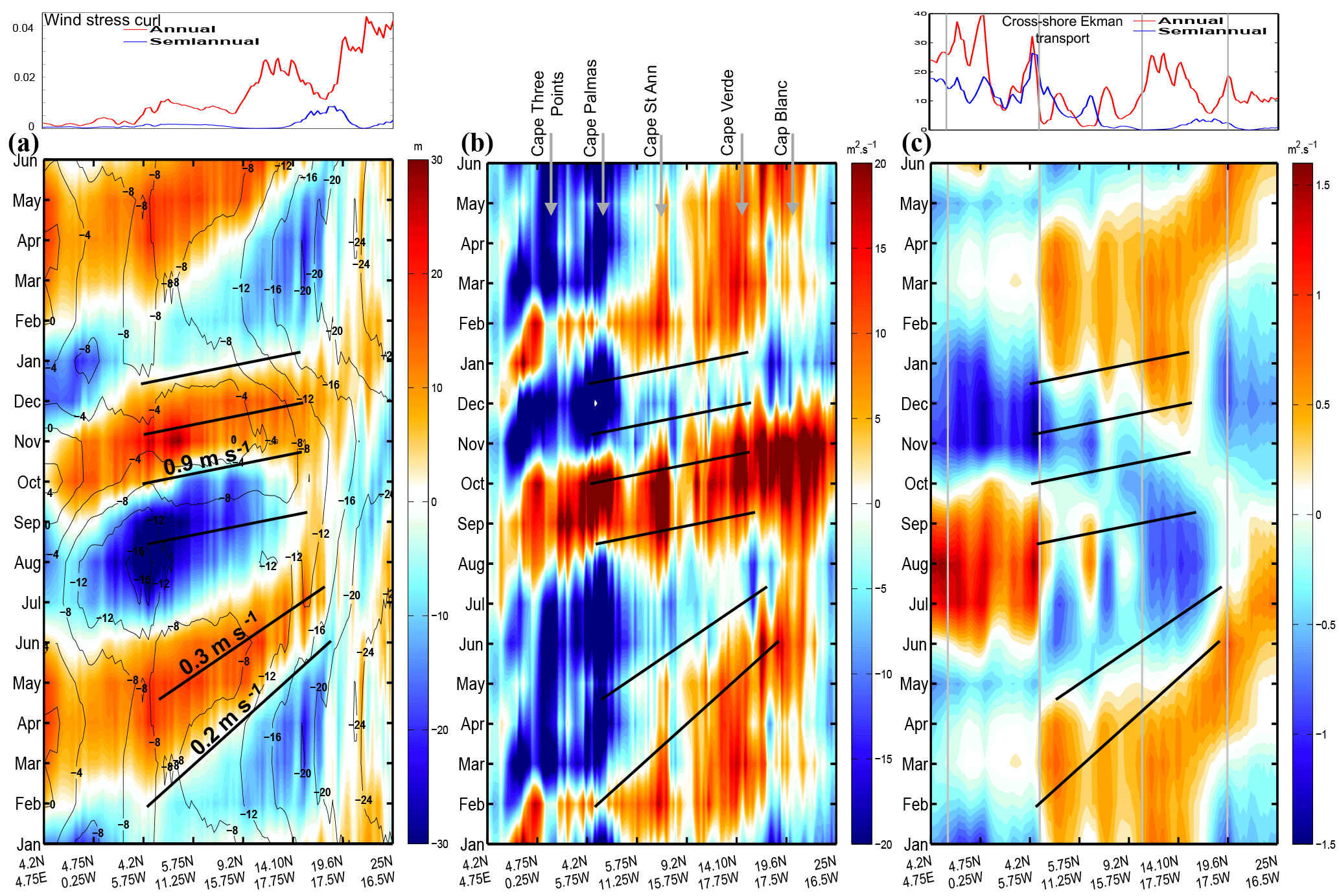
Figure 12Time–along-slope distance diagram following the 100 m isobath (see location in Fig. 1) for the TROP025 climatological seasonal cycle of (a) the depth anomaly of the 18∘ isotherm δz18 (colors; in meters) and SLA (contours; cm), (b) along-slope geostrophic transport between σt=26.7 and the surface (m2 s−1), and (c) across-shore Ekman transport anomaly. Oblique solid black lines correspond to propagation speeds of 0.2–0.3 (February–June) and 0.9 m s−1 (August–January). They are subjectively drawn in (a) (and repeated in b and c) to indicate where spatiotemporal patterns are suggestive of along-slope propagation. In panel (c), vertical gray lines delineate the sectors over which sector upwelling indices are computed (see Fig. 13). Power spectral densities associated with the annual and semiannual harmonics of the wind stress curl and cross-shore Ekman transport along the 100 m isobath are displayed above (a) and (c), respectively.
The significance of semiannual fluctuations has been established for the circulation of several regions of the equatorial and tropical ocean (Clarke and Liu, 1993). In a nutshell, this arises from having the ITCZ pass twice a year over these regions. The central and eastern equatorial Atlantic receives significant semiannual forcing from the winds (Busalacchi and Picaut, 1983). Variability at this frequency is further enhanced by abrupt temporal changes in zonal winds (Philander and Pacanowski, 1986) and basin-mode quasi-resonance (Brandt et al., 2016; Ding et al., 2009). The equatorial response can then be propagated poleward along eastern boundaries by coastal trapped waves, as occurs in the northern and southern Pacific (Gómez-Valdivia et al., 2017; Ramos et al., 2006), for instance. The Northern Atlantic is peculiar in that coastal trapped waves generated by the reflection of equatorial Kelvin waves in the eastern Gulf of Guinea (GG) have to propagate along a long and corrugated stretch of coastline to reach WA latitudes, with a significant part of the coastline being situated on the edge of the equatorial band at ∼4∘ N. This basin geometry is not prone to the coastal transmission of equatorial signals (Philander and Pacanowski, 1986; Polo et al., 2008). Despite some controversies, several studies have dismissed a connection between the equatorial region and the northern GG (Clarke, 1979; Houghton, 1983). To gain further insight into the possible remote sources of semiannual poleward flow off WA, we computed time–along-slope distance diagrams (i.e., following the continental slope) for the climatological cycle of 18∘ isotherm depth anomalies (δz18, a proxy for thermocline depth anomaly) and anomalies (Fig. 12). The along-slope coordinate covers from 4.2∘ N, 4.75∘ E (inside the GG) to 25∘ N, 16.5∘ W. A diagram for climatological anomalies of across-shore Ekman transport is also presented.
Overall, we observe clear signs of long-range poleward propagation for thermocline depth and along-slope flow but this assertion should be qualified for the following reasons: (1) propagation is more clearly visible for δz18 than for (which is considerably noisier) and sea level anomaly (SLA; contours in Fig. 12a) ; (2) propagation is more evident during Pf than Ps, with distinct time–space patterns for the two periods; (3) examination of Fig. 12 reveals an off-equatorial maximum in poleward flow and thermocline depression in the longitude range 4–14∘ W (i.e., in the GG) with no clear connection to the area east of 0∘ W; (4) the temporal lag between thermocline depth anomaly (δz18) and geostrophic velocity () seasonal fluctuations is not consistent with Kelvin wave theory; and (5) propagation becomes increasingly ambiguous north of Cape Verde at ≈15∘ N.
To help with the discussion of reasons (2) and (3), Fig. 13 displays the seasonal cycle of the upwelling index (i.e., Ekman transport) integrated over the stretch of coastline between 3∘ E and 7.5∘ W:
where α is the angle between the north and the tangent to the coastline leaving land on the right and s is the curvilinear coordinate following the 100 m isobath. UIWAC (UIWA) is similarly defined for the longitude (latitude) band 7.5–17∘ W (10–20∘ N), corresponding to the “West African corner” between Cape Palmas and Cape Roxo (West Africa between Cape Roxo and Cap Blanc; see Fig. 1 for locations). All three sectors are of comparable length.
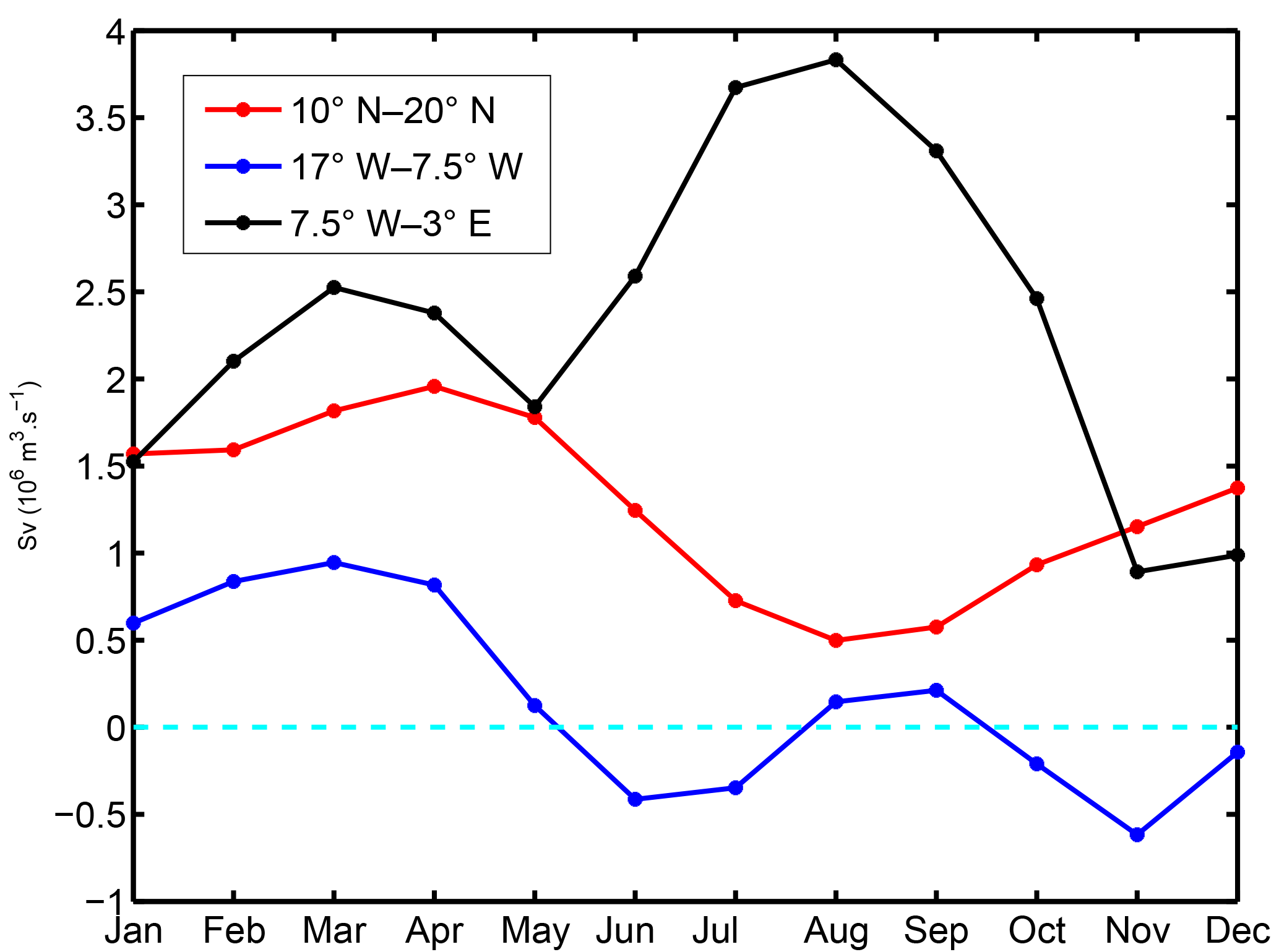
Figure 13Monthly mean climatology of across-shore Ekman transport (Sv) integrated along the 100 m isobath for three sectors: in the Gulf of Guinea between longitudes 3.5∘ E and 7.5∘ W (black; GG), further west between 7.5 and 17∘ W (blue; WAC), and between 10 and 20∘ N (red; WA). The position of these sectors, which are of comparable length, is indicated in Figs. 1a and 12c.
Reason (1) is partly expected because along-slope velocities associated with coastal trapped waves should be approximately geostrophic, and hence they depend on the across-shore derivative of δz18 (Cushman-Roisin and Beckers, 2011). Note also that standing meanders of the WABC past topographic irregularities can produce substantial excursions of the flow away from the shelf break and hence rapid along-slope changes of (see Fig. 10; the position in the main capes is indicated in Fig. 12). The lack of clear propagation tendency found for SLA was previously noticed by Polo et al. (2008) and reflects the fact that sea level over the slope area is at least partly decoupled from δz18 (and also from ). This limits the utility of altimetry to investigate remotely forced dynamics off WA.
Regarding reason (2), we note that south of 15∘ N a propagation phase speed can be identified with reasonable confidence during Pf, especially for δz18. We estimate c at ≈ 0.9 m s−1 in Fig. 12a and this value is also applicable to . This is compatible with low vertical-mode coastal trapped wave propagation and, more importantly, consistent with the propagation speed inferred by Picaut (1983) for the GG coastal upwelling signals (0.7–0.8 m s−1).3
On the other hand, the coherence of the signals expected from poleward propagation is weaker around Ps, especially for . Even for δz18 propagation speed is ambiguous and seems to change with time (≈0.2 m s−1 at the transition between negative and positive δz18 anomalies but a bit faster toward the downwelling peak (∼0.3 m s−1), which roughly coincides with a sign change of north of Cape St Ann (Fig. 12). Such values are untypical for coastal trapped waves. The slow northward shift of the downwelling signal (negative δz18 and strong poleward flow) may alternatively be attributed to the progressive seasonal migration of the upwelling wind region (related to the seasonal displacement of the ITCZ) but the correspondence between panels (a), (b), and (c) in Fig. 12 is only partially supportive of this. In addition, propagation at ≈0.9 m s−1 may also be present, e.g., toward the end of Ps in May. This suggests that both local and remote responses to winds combine to produce the winter–spring WABC intensification. Examination of Fig. 13 reveals a complex picture in which each separate coastal sector contributes to Ps upwelling relaxation over a slightly different time period: April to August for WA; March to June for WAC; and March to May for GG. Also note that the GG relaxation is immediately followed by marked increasing upwelling tendency from May to July. Overall, forcings over the different sectors largely oppose each other; hence the weakness of propagating oceanic signals and perhaps also the weakness of the poleward flow relative to Pf.
With respect to Pf and reason (3), our analyses suggest the existence of a remote origin for the WABC intensification off WA, with an evident off-equatorial maximum in poleward flow and thermocline depression in the longitude range 4–14∘ W, i.e., in the GG (Fig. 12). For the period October–December, the largest positive values are found in this longitude range. On the other hand, Hovmüller diagrams for δz18 and exhibit some pattern changes at ≈0∘ W near the left edge of Fig. 12. We take this as an indication that the equatorial region is not implicated in the generation of the Pf CTW signal4. Examination of 2-D monthly regional maps for δz18 (not shown) confirm the absence of oceanic signal propagation between the Equator and the northern part of the GG. Figure 13 confirms the importance of the GG sector as a forcing region for poleward flow during Pf. An abrupt upwelling relaxation takes place in the GG from August to November when the ITCZ approaches and passes over this sector (Schneider et al., 2014). This relaxation is far steeper than the boreal winter one (compare the two drops in upwelling index UIGG in Fig. 13 and the corresponding local thermal response in Fig. 6 and Picaut, 1983, his Fig. 15b). To our knowledge, there has been no previous mention of the role played by the GG wind cycle as a source of remote forcing for the poleward flow in the southern part of the Canary Current system (although remote forcing from equatorial origin has been invoked to explain the seasonal cycle of subsurface temperature off Dakar; Busalacchi and Picaut, 1983; McCreary et al., 1984). UIWAC also decreases during Pf, so winds in the WAC sector must contribute to WABC intensification, but the amplitude of the relaxation is smaller by a factor close to 4. The relative importance of the remote forcing associated with each sector depends on their along-slope decay scale, which is poorly constrained and may depend on a number of factors. Limited insight into this question can be gained by comparing Pf and Ps remote forcings.
During Ps the WAC wind relaxation is about twice as intense as during Pf and combines (between April and June) with the local relaxation of WA winds. However, the ocean response in terms of poleward flow is significantly weaker than the one during Pf both in terms of current magnitude and meridional extent. GG winds are thus plausibly instrumental in driving the model WABC intensification in fall and, conversely, opposing intensification during most of Ps. Further analyses will be needed to clarify this because the seasonal cycle of other environmental parameters may also be involved, e.g., the near-surface density gradient along the waveguide, which is larger in spring than in fall (Fig. 9).
With respect to reason (4), δz18 and are not precisely in phase as they are expected to be for theoretical Kelvin waves in a model for a single baroclinic mode (Cushman-Roisin and Beckers, 2011). A phase shift of the order of 1 month exists between the two variables with δz18 lagging; i.e., Pf poleward flow intensification initiates while the thermocline is still in an uplifted position (Fig. 12). A similar discrepancy has been noted before for the California undercurrent and attributed to the effects of Rossby waves dynamics (Oey, 1999). Radiation of Rossby waves from the coastal waveguide implies that pressure disturbances associated with CTW dynamics propagate offshore. In turn, this modulates the along-slope flow, which depends on the nearshore–offshore pressure difference. In particular, this produces a phase lead for compared to the thermocline depth at the coast (Oey, 1999). We will discuss the Rossby wave activity offshore of WA in the next section and add support to this explanation.
With respect to reason (5), the propagation of thermocline depth anomalies associated with Pf becomes progressively elusive beyond Cape Verde5. This would not be inconsistent with the major influence exerted by this cape on the poleward flow (Alpers et al., 2013; Capet et al., 2017) and its dispersive effect on coastal trapped waves (Crépon et al., 1984). The area located between 15 and 20∘ N (i.e., Cape Verde and Cap Blanc, respectively) is also characterized by a rapid shift in the dominant periodicity of δz18 and fluctuations (Figs. 11 and 12) from semiannual to annual. In particular, δz18 variability becomes increasingly complex with reduced magnitude when approaching Cap Blanc where upwelling is permanent. Overall, TROP025 suggests the existence of a transition in this latitude range despite the fact that the WABC can be present up to ∼25∘ N in fall.
Overall, no significant forcing in a semiannual period is present north of Cape Palmas (see frequency decomposition of across-shore Ekman transport in Fig. 12) and our analyses indicate that the WABC seasonal cycle is made of two parts that are distinct in terms of forcing mechanism. The strongest poleward flow intensification occurs in fall, both in terms of flow speed and also poleward extent (25∘ N vs. 20–22∘ N in the model). Such differences seem consistent with existing WABC observations (see Sect. 7) and presumably reflect the strength of remote forcing processes. In fall, poleward flow intensification has been related to a major upwelling wind relaxation in the Gulf of Guinea. In contrast, Ps flow intensification appears to be a more complex combination of local and remote responses with time lags resulting in partial compensations.
As presented above, the across-shore structure of the WABC and its seasonal evolution are strongly suggestive of the important role played by westward Rossby wave propagation. So is the seasonal evolution of the meridional flow patterns that increasingly tilt away from the north–south axis in a clockwise manner as they progress westward (Fig. 10) owing to the rapid change in Rossby wave phase speed in the tropics (Chelton and Schlax, 1996). More precisely, Figs. 7, 8, and 10 are consistent with the generation of semiannual Rossby waves at the WA eastern boundary via the scattering of coastal waves due to the meridional gradient of the Coriolis parameter (McCalpin, 1995; Ramos et al., 2006). Elements of linear theory are recalled first as a starting point (Cushman-Roisin and Beckers, 2011). Assuming no meridional structure to the wave, i.e., the horizontal wavenumber is , the Rossby wave dispersion relation is
where Rn is the deformation radius for a given vertical mode n. Rn can also be expressed as a function of the gravity wave speed cn for that mode: . The (zonal) phase speed of a monochromatic wave of frequency ω and zonal wavenumber k is thus
More complex perturbations propagate at the group velocity
Finally, for a given deformation radius and wave period there is a critical latitude λn(ω) beyond which the free Rossby wave mode is evanescent because the associated wavenumber solution to the quadratic Eq. (6) has a nonzero imaginary part. At this critical latitude so λn is defined by the fact that where RT is the Earth radius.
In what follows baroclinic mode characteristics are determined based on the TROP025 stratification computed on the model 75 grid levels. The calculation is made with the dynmode program available at https://woodshole.er.usgs.gov/operations/sea-mat/klinck-html/index.html (last access: 18 August 2018). Using the gravity phase speeds computed at 14∘ N and indicated in Fig. 16, we find 22, 11, and 7∘ N for the critical latitudes corresponding to the semiannual frequency and vertical modes 1, 2, and 3, respectively. These estimates are in good agreement with those of Clarke and Shi (1991). The gravity phase speed of mode 3 is slightly higher around 7∘ N than at 14∘ N (0.85 m s−1 at 8∘ N vs. 0.70 at 14∘ N), so a more accurate estimation of λ3 is 9.5∘ N.
Table 2Parameters associated with each potential semiannual RW mode at 8 (baroclinic mode 1 to 3) and 14∘ N (baroclinic mode 1 and 2). Gravity phase speed (m s−1), deformation radius (km), critical latitude (km), theoretical wavelength (km), observed TROP025 wavelength (km), theoretical phase speed (cm s−1), theoretical group velocity (cm s−1), and observed TROP025 propagation speed (cm s−1) are reported. No mode 1 RW is identified at 8∘ N. A mode 2 RW is also not identified at 14∘ N, in agreement with linear theory predicting its evanescence. Note the important discrepancies between theory and model RW mode 1 at 14∘ N.
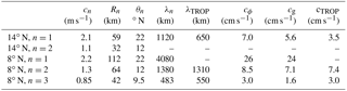
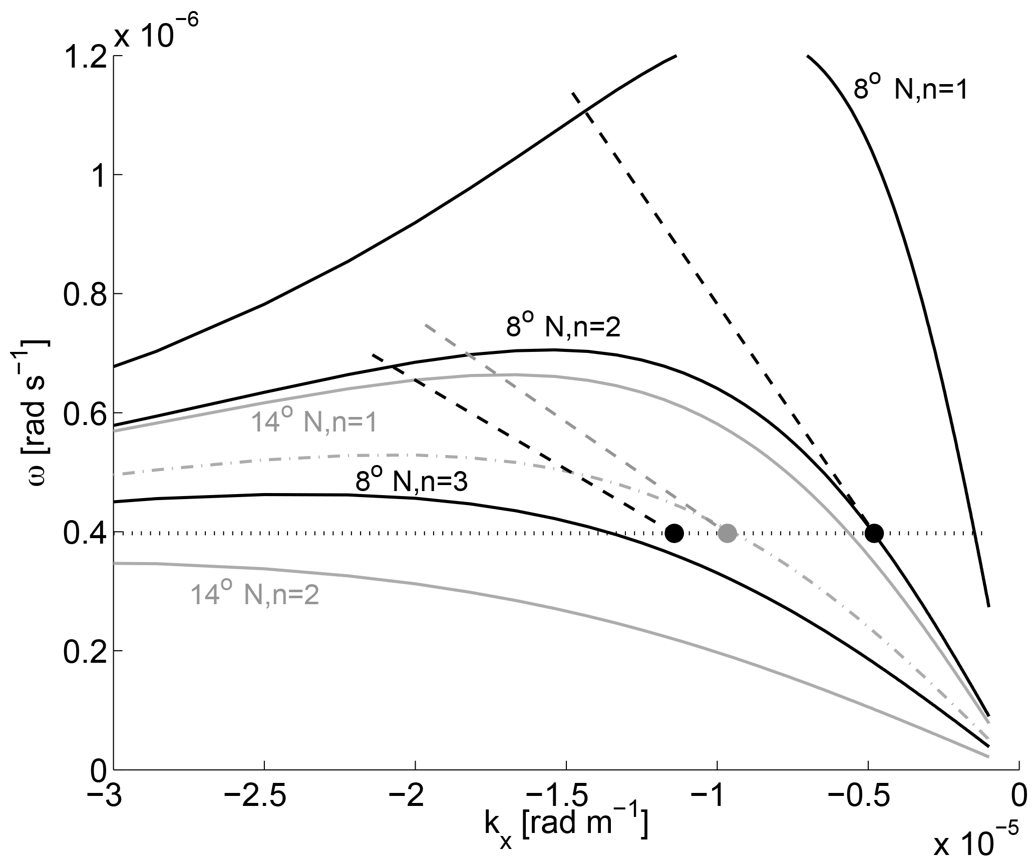
Figure 14Wavenumber–frequency dispersion diagram for baroclinic Rossby waves corresponding to values of the deformation radius equal to 112, 64, and 42 km (solid black, baroclinic modes 1–3 at 8∘ N) and 59 and 31 km (solid gray, baroclinic modes 1 and 2 at 14∘ N). The black (gray) filled dots and dashed lines represent the Rossby wave characteristics identified in Fig. 8 for TROP025: ω=2 π/(6 months); and cTROP as listed in Table 2. The gray dash-dotted line is the dispersion curve that passes through the Rossby wave mode identified at 14∘ N in TROP025. Its associated deformation radius is 48 km, i.e., significantly less than the actual baroclinic mode 1 deformation radius at that latitude (59 km). The horizontal dotted line corresponds to the semiannual frequency.
Our aim is now to describe the semiannual Rossby wave dynamics present in TROP025, assess the degree to which the simplest linear theory captures this dynamics, and gain insight into the different baroclinic mode contributions. Dispersion diagrams are shown in Fig. 14 for the Rossby wave modes permitted at 8 and 14∘ N, modes 1 to 3 for the former and mode 1 for the latter. The dispersion curve for mode 2 at 14∘ N is also shown. The fact that it does not intersect the horizontal line corresponding to semiannual frequencies underscores the evanescent nature of mode 2 RWs at this latitude. Model wavenumbers and propagation speeds deduced from careful examination of Fig. 8 are reported in Fig. 14. At 8∘ N a slow and a fast wave coexist. They fall quite accurately on mode 2 and 3 dispersion curves, respectively. On the other hand, the dominant wave identified at 14∘ N is distinct from a linear mode 1 RW (see also Table 2).
To elaborate on the significance and relative importance of the different RW modes, a harmonic analysis was performed at each grid cell () over the period 1982–2012 to extract the semiannual variability of the meridional velocities. The resulting semiannual harmonics (6-monthly values) were subsequently decomposed onto the baroclinic modes computed for each location (xi, yj) based on a local annual mean profile of Brunt–Vaisala frequency. Horizontal maps of the depth-integrated kinetic energy associated with modes 1–4 are shown in Fig. 15, after time averaging over the semiannual cycle. Restricting the final step of vertical integration to the layer in which the poleward flow is concentrated, e.g., the upper 200 m, leads to similar results and conclusions. The dominance of mode 2 is a well-known attribute of many equatorial and tropical regions (Philander and Pacanowski, 1980). Mode 2 dominates over most of the ETNA except for a few isolated offshore grid cells in the latitude range 10–15∘ N where mode 1 is of comparable magnitude. The shape of the region having finite values of mode 2 kinetic energy and the general offshore decay seen in Fig. 15b are consistent with the following: energy being mainly radiated from the coastal waveguide where the largest energy values are found; and westward energy propagation being more effective at lower latitudes and ineffective north of 12–15∘ N, with a noticeable change in the cross-shore size of the region with finite energy values around 10∘ N. A similar impression can be drawn for mode 3 and 4 except that westward propagation seems both more strongly damped and more confined meridionally in a low-latitude band. This is qualitatively consistent with the λn values decreasing with mode order (Table 2). The kinetic energy distribution for mode 1 is peculiar and does not exhibit large values in the coastal waveguide (Fig. 15a). Why so little of the semiannual CTW activity projects onto baroclinic mode 1 is a pending question left for a future investigation.
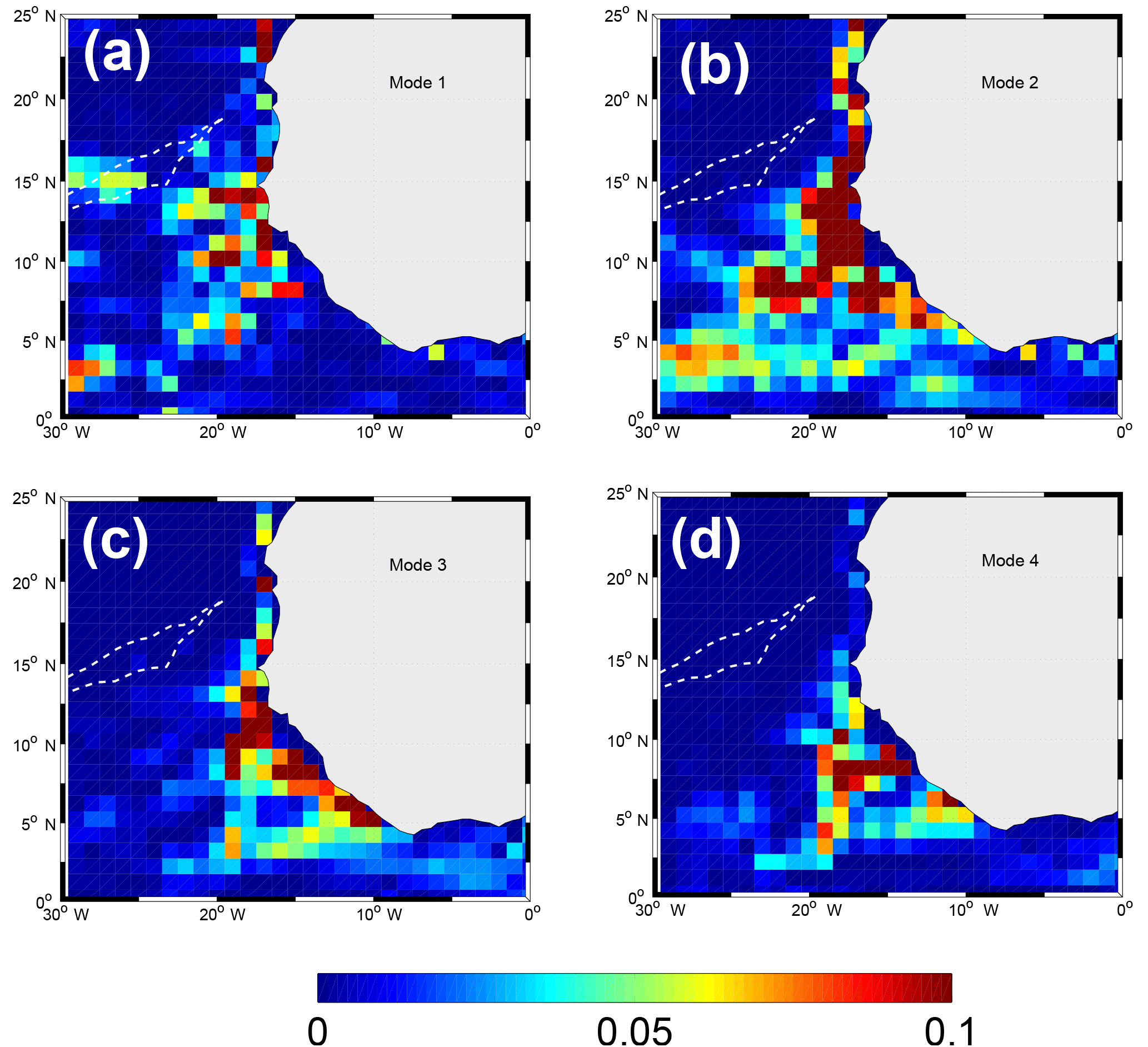
Figure 15Vertically integrated kinetic energy (m3 s−2) for the semiannual meridional velocity decomposed onto baroclinic modes. Only the first four modes are shown. Time averaging is performed over the semiannual cycle. The two white dashed lines represent the location where zero PV gradients are found in Fig. 17.

Figure 16Vertical structure of the ETNA baroclinic modes 1 (blue), 2 (green), and 3 (red) for pressure and horizontal velocities (upper 2500 m only). Calculation is made using TROP025 stratification at 14∘ N, 18∘30′ W. The associated reduced gravity phase speed ce ( s−1) for each mode is also indicated.
Westward propagation of energy away from the coastal guide is an important process contributing to the poleward attenuation of the WABC. Over the continental slope, the progressive deepening of the WABC with increasing latitude (Fig. 9) corresponds to a reduction (increase) in the relative contribution of high-order (low) modes, e.g., less weight on mode 3 whose upper zero crossing is at 75 m (Fig. 16). Although this is consistent with idealized simulations and theoretical arguments (McCreary, 1981; Philander and Yoon, 1982), we cannot be certain that TROP025 motions associated with high-order modes along WA are more efficiently damped for physical reasons (such as RW generation and frictional processes) as opposed to being dissipated by excessive numerical viscosity and/or diffusion. For a given mode n dissipation of numerical origin should increase as latitude increases and the corresponding typical horizontal scale associated with that mode Rn decreases. The realism of the model WABC may thus deteriorate with increasing latitude.
In this context, the model behavior in the latitude range ∼14–22∘ N requires further clarification. The northern end of this sector coincides with the critical latitude for baroclinic mode 1 semiannual RWs; hence the possibility of resonant excitation of these waves because their group velocity vanishes (Hagen, 2005). On the other hand, Hovmüller diagrams similar to Fig. 8 for latitudes between 15 and 22∘ N reveal a dramatic reduction of the semiannual RW signal toward the north (not shown but see Figs. 10 and 15 for indirect evidence). This latitude range corresponds to a major transition in the Canary Current system with distinct WSC forcing conditions and dynamical regime on either side (offshore conditions associated with negative wind stress curl and equatorward flow prevail north of 20∘ N), two abrupt geomorphological near discontinuities (at Cape Verde and Cap Blanc), and the permanent Cape Verde thermohaline frontal zone. All these sources of nonlinearities can contribute to the northward weakening of the semiannual CTW signal and thus prevent the generation of semiannual RW activity beyond 18–20∘. They can also explain the discrepancies found at 14∘ N between RW characteristics expected from linear theory and those identified in the model.
However, the upper ocean potential vorticity (PV; see Sect. 2) field offers another compelling explanation for the meridional structure of the RW field found in TROP025. Equation (6) is strictly valid in a large-scale ocean at rest in which the only source of background PV gradient is the Coriolis parameter gradient . In realistic conditions, the large-scale PV field implicated in the propagation of baroclinic Rossby waves must account for stretching effects associated with background shear flows if any (Killworth, 1979; de Szoeke and Chelton, 1999). More appropriate quantities to investigate upper ocean RW dynamics are total PV gradients in three density layers (see definition in Sect. 2): 25.2–26.3 (layer 1), 26.3–26.7 (layer 2), and 26.7–26.9 (layer 3). Layers 1 and 2 are layers in which a large fraction of the WABC transport is concentrated (Fig. 9). They are of comparable thickness and typically occupy the upper 200–250 m. Layer 3 is also of comparable thickness but it is associated with a modest fraction of the poleward transport, both nearshore (Fig. 9) and offshore (Fig. 7). PV fields calculated following Eq. (4) are shown in Fig. 17 as is their gradient vector field. Layers 1 and 2 exhibit relatively similar patterns. PV gradients in these layers strongly depart from those resulting from variations in the Coriolis parameter alone. In particular, a reversal of the gradient is found along oblique lines that run northeast to southwest between Cap Blanc and the Cape Verde islands. RWs approaching these lines must be subjected to intense dispersive, refractive, and/or dissipative effects. Layer 3 is the deepest layer where PV gradients are not uniformly oriented toward the north (the gradients vanish in a broad northern sector where stratification and Coriolis parameter contributions nearly cancel). Below layer 3 PV gradients are dominated by β and relatively uniform from the coast to thousands of kilometers offshore (not shown).
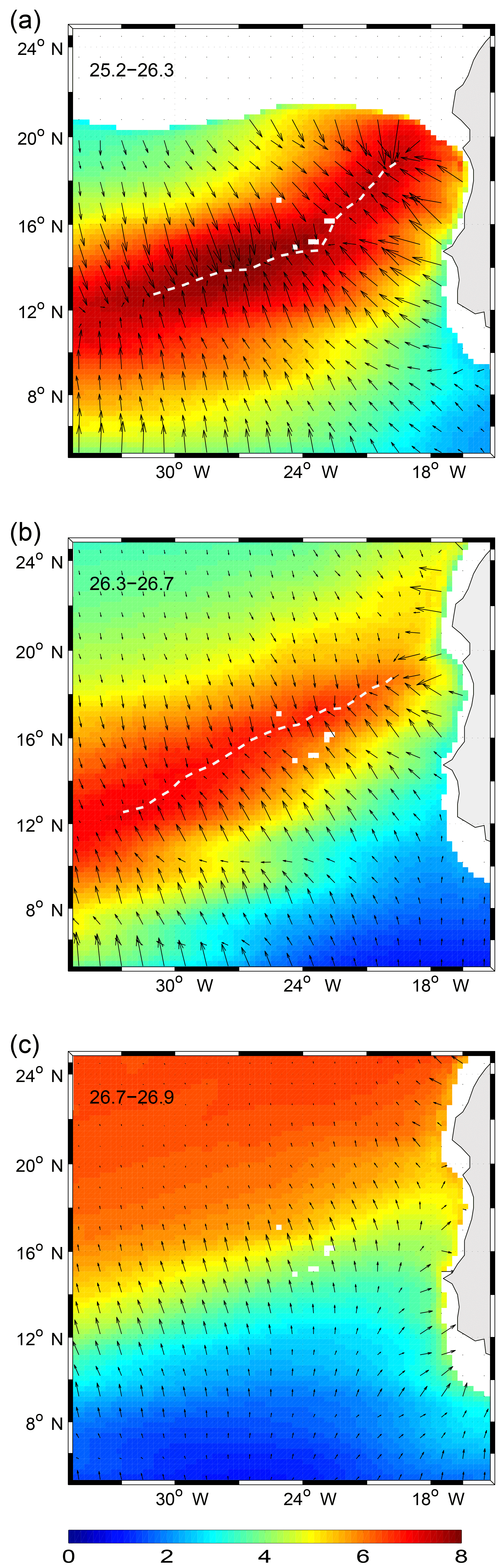
Figure 17Shallow-water potential vorticity field in the ETNA computed from TROP025 (color; 10−8 m−1 s−1) using Eq. (4) for the density classes 25.2–26.3 (a), 26.3–26.7 (b), and 26.7–26.9 (c). These values are such that the three layers are of comparable thickness and the same color scale can be used. Potential vorticity gradients are also shown in vectors. Note the vanishing gradients found along the white dashed lines in panels (a) and (b) (the position of the two lines differ slightly, e.g., see their position with respect to the Cape Verde islands).
At 14∘ N, the zero PV gradient line in layer 1 (layer 2) is located at ∼24∘ W (28∘ W) so the distance to the WA shelf break is not enough (marginally enough) to fit a linear RW wavelength (λ1=1120 km; see Table 2) in the sector where PV gradients are mainly directed from south to north and relatively uniform spatially. We suspect that the differences in PV gradients between layers 1–2 and the deeper layers are implicated in the deviations from standard linear theory (wavelength and propagation speed) and also in the rapid RW signal attenuation observed within 1000 km from shore (Figs. 8 and 15) despite the critical latitude being located far to the north. Importantly, the width of the sector situated east of the zero PV gradient decreases rapidly with latitude between 14 and 20∘ N and is only ∼300 km wide at 18∘ N. This makes the existence of long weakly dispersive semiannual RWs increasingly implausible when approaching Cap Blanc.
Overall, the modifications of the ETNA PV field by vortex stretching effects in the density range 25.2–26.7, at which most of the meridional flow and Rossby wave energy are concentrated, appears as a good candidate to explain the (meridionally variable) cross-shore damping scale for RWs and the progressive reduction of RW amplitude north of 15∘ N. At deeper depths, the impact of the PV gradients in the upper ETNA may be more limited. Across-shore sections reveal alternating bands of poleward and meridional flow below 300–400 m that migrate westward past the zero PV gradient lines identified above (not shown), suggesting the presence of Rossby wave activity there in agreement with the observational findings of Hagen (2001). The physical processes responsible for the particular PV structure present in the upper ETNA will be discussed in Part 2.
Excitation of free Rossby waves by wind stress curl forcing along WA can also contribute to RW activity and in turn impact the WABC seasonal cycle. This is expected to arise if the WSC spatiotemporal patterns of variability in the immediate vicinity of WA involve particular wavenumber–frequency pairs consistent with the dispersion relation of free RWs (White, 1985). South of 20∘ N, the wind stress curl and Sverdrup transport fields shown in Fig. 1 exhibit across-shore spatial variations with a contribution of wavelengths 500–1500 km. This is in the appropriate range to excite baroclinic mode 1 and 2 RWs south of their critical latitude. But semiannual variability of the wind curl signal is particularly weak in the WA sector (see Fig. 12) so its contribution to the WABC semiannual cycle must be limited. Based on frequency considerations the generation of an annual RW signal is more plausible. However, a harmonic analysis similar to the one described above reveals small amounts of energy associated with the annual cycle of the upper ocean meridional flow (not shown). We relate this to a combination of inhibiting factors. South of 15∘ N mode 1 RWs have wavelengths ∼ 2500 km or more, i.e., too large to be compatible with the WSC typical spatial scales of variability. North of 10–12∘ N such RWs are also too large to fit in the sector situated east of the line where PV gradients vanish.
An eddy-permitting numerical simulation with realistic forcings has been analyzed to investigate the dynamics of the boundary current along the West African seaboard. The depth range of interest was chosen to be above the σt=26.7 isopycnal. This broadly coincides with the upper 250 m of the water column and places the focus on the layer of fluid in which the wind-driven circulation is overwhelmingly concentrated. The geographical focus is roughly on the southern sector of the Canary Current system between ∼8 and 20∘ N. In this area wind stress curl (both nearshore and offshore) is robustly positive, i.e., conducive to poleward flow6. In fact, upper ocean equatorward currents are rarely found over the WA continental slope, except when approaching 8–10∘ N where WSC is much reduced. The model poleward flow is characterized by two main intensification periods in spring and fall. We interpret this characteristic as a consequence of the low-frequency coastal trapped wave activity generated locally and remotely by seasonal wind fluctuations along the African shores7. This is an important difference from the annual cycle of the boundary slope current discussed in several past studies including Mittelstaedt (1991) and Lázaro et al. (2005). Note, though, that important signs of a semiannual cycle can be seen in Lázaro et al. (2005) in which two along-slope transport maxima are found across their so-called section B.
Despite some differences in their forcing regions and precise depth–latitude range of influence, the spring and fall model WABC intensifications bear important similarities. They are both part of a semiannual cycle whose forcing processes were carefully investigated. We found no clear signs that along-slope motions in the form of free Rossby wave modes could be excited by nearshore WSC, perhaps because the WSC temporal variability at semiannual frequency is particularly small. Conversely, along-slope flow generation and propagation in the coastal waveguide is prominent as we found throughout the study. Considered in isolation, the WABC spring intensification accompanies the relaxation of wintertime coastal upwelling winds in the latitude range 7–20∘ N as the ITCZ shifts northward toward that area. Flow intensification is found in the subsurface and is broadly consistent with the theory on undercurrents in upwelling systems. Time lags between the contributions of the wind for different sectors along the African coast are such that compensating effects occur and the WABC forcing is suboptimal. The fall intensification is stronger. It has a more remote and focused origin that we are able to locate in the Gulf of Guinea through spatiotemporal analyses of both wind forcing and coastal ocean response. Owing to this remote forcing, the largest WABC transports occur while WSC is relatively weak and upwelling winds intensify, i.e., when local forcing is least conducive to poleward currents. In that respect, our work tends to substantiate old assertions about the connection between the boundary current flowing offshore of Senegal and Mauritania as well as poleward flow in the Gulf of Guinea, albeit only during part of the annual cycle. Conversely and in contrast to what has been hypothesized for the southeast tropical Atlantic (Rouault, 2012; Schouten et al., 2005), wind variability and Kelvin wave activity in the equatorial Atlantic are not found to be implicated in the forcing of the WABC semiannual cycle (McCreary et al., 1984). Our results also differ from those for the eastern South Atlantic (Junker et al., 2015) in that the seasonal cycle of the WABC is not directly linked with the local wind stress curl, which as mentioned above has very little semiannual modulation.
More quantitatively, the model provides estimates for poleward transport over the WA continental slope. They depend somewhat on the precise choices made for the control surface (depth, across-shore integration bounds, and position in latitude). At the latitude of Senegal (Mauritania), geostrophic transport above σt=26.7 is of the order of 1 Sv (0.4 Sv), i.e., a large (moderate) fraction of the theoretical barotropic Sverdrup transport. We relate this to the meridional changes in WABC dispersion through Rossby wave generation. Indeed, dispersion is most pronounced at low latitudes where Rossby waves travel faster and higher baroclinic modes can be impacted. The vertical structure of the boundary currents reflects these differences. Upper ocean confinement of the Sverdrup flow by Rossby waves (Anderson and Gill, 1975; Philander and Yoon, 1982) is systematically most pronounced at lower latitudes; hence the north–south differences in depth range of the WA boundary current. Transport distribution at 8∘ N is also consistent with these assertions but WSC diminishes greatly when approaching such low latitudes where our analyses may be more difficult to interpret.
The model analysis of Rossby wave activity reveals important differences from previous descriptions of these waves at larger scale in the eastern to central North Atlantic (Hagen, 2005). Most notably, we find that upper ocean Rossby wave activity generated at the eastern boundary remains confined to a well-defined ocean sector delimited by the WA seaboard and an oblique line running northeast–southwest where background potential vorticity gradients vanish in the upper ocean. Such modification of the potential vorticity field is due to stratification effects having a magnitude comparable to planetary vorticity effects (β). Past studies of Rossby wave activity in the North Atlantic have classically been made using linear 1.5 layer reduced gravity models (Busalacchi and Picaut, 1983; Da Silva and Chang, 2004; Garzoli and Katz, 1983) with no background flow that RWs can interact with. It seems to be an important limitation for the ETNA sector situated north of about 12∘ N.
Our main qualitative conclusions on the processes responsible for the WABC semiannual cycle and its associated RW dynamics in our model are schematically summarized in Fig. 18. The relevance of this numerical investigation to the real WA ocean is an obvious concern. Although TROP025 skills at regional and basin scale have been demonstrated (Sect. 2) model biases cannot be excluded at the scale of the WABC. Because there have been relatively few observational programs in this part of the world ocean we can only offer limited and qualitative insight into model realism, for example on the reality of the two WABC intensification phases and the associated flow characteristics. Although the existence of two poleward intensification phases is not systematically recognized in previous studies, published observations are not inconsistent with the model behavior, including on the timing of these two phases.
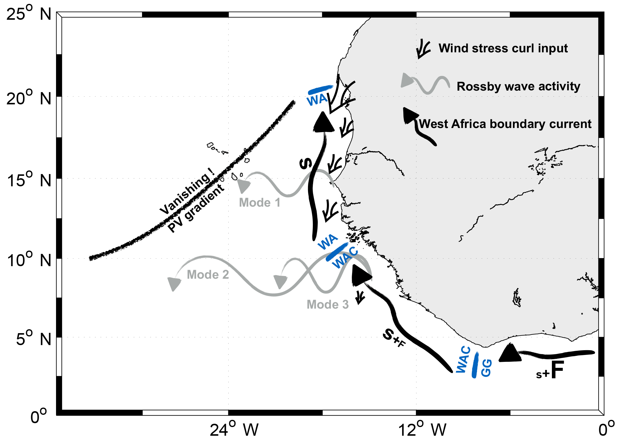
Figure 18Schematic representation of the main processes relevant for the WABC seasonal cycle as identified in this study. Two WABC intensification phases occur in spring (S) and fall (F) in relation to the relaxation of cross-shore Ekman transport along different sectors of the African coast. The relative importance of each sector varies depending on the season. The font size of the S and F letters next to the WABC arrows is indicative of this importance. Three sectors are distinguished: the Gulf of Guinea (GG), the West African corner (WAC), and West Africa (WA). The fall intensification is mainly due to wind changes in the GG and a modest contribution from the WAC. The spring intensification is the outcome of a subtle combination of forcings in all three sectors with a prominent role of local WA forcings. The spatiotemporal variability of the wind stress curl forcing does not have an appreciable effect on the WABC seasonal cycle, although it is a key local determinant of the climatological mean meridional transport along WA (weak near 8–10∘ N and particularly strong near 20∘ N). The WABC is subjected to scattering and gives rise to Rossby wave (RW) activity hundreds to thousands of kilometers offshore. The characteristics of these RWs exhibit rapid meridional changes over a few degrees of latitude. At low latitude (∼8) where β is largest RWs associated with baroclinic modes 2 and 3 dominate. At 14∘ N where only mode 1 RWs are permitted the model RWs significantly differ from those predicted by standard linear theory. This discrepancy and the progressive disappearance of RW activity north of 15∘ N may be related to the peculiar structure of the upper ocean ETNA PV field: above approx. 250 m of depth the gradient of the background PV field (β + stratification effects) vanishes along a line running northeast to southwest.
The field experiment CANOA08 took place in November 2008 at a time of year when the poleward flow should be most intense including near the surface. Above σt=26.85 the flow over the continental slope carried SACW up to 25∘ N (Peña-Izquierdo et al., 2012) where vanishing meridional transports were found, i.e., exactly the November climatological limit determined for the same density class in the model (not shown). In addition, observed transports are broadly consistent with those found in TROP025, particularly for the uppermost stratum examined by Peña-Izquierdo et al. (2012) (see model–data comparison in Table 3). In CANOA08 the intense poleward surface and subsurface currents found in the vicinity of Cap Blanc at surface and subsurface levels are interpreted by the authors as, respectively, “a late expression of the summer Mauritania current” and a local response to strong upwelling winds (Peña-Izquierdo et al., 2012). Our model results cast doubt on these interpretations and suggest instead that CANOA08 may have sampled the ETNA at the (normal) time when the fall intensification of the surface and subsurface WABC is remotely forced.
Table 3Meridional transports observed in November 2008 reported in Peña-Izquierdo et al. (2012) (left) and their TROP025 climatological equivalent for the month of November (right) separated by the / symbol. Transport values (in Sv) are provided for two different density layers (SW for surface waters, σt<26.46; uCW for upper central waters, 26.46<σt<26.85) and four latitudes (16.25, 17.5, 20, and 24∘ W). In situ values are estimated visually from Fig. 7a–c in Peña-Izquierdo et al. (2012) for the cross-sectional area between the shelf break to 60 km offshore. For the model, transport is computed over four grid cells (100 km) situated offshore of the shelf break. Using this wider across-shore section is meant to account for our limited horizontal resolution, but transports estimated over only three grid cells only differ by 15 %–20 %.
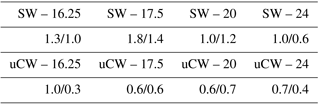
On the other hand, comparison with CANOA08 observations raises some concerns about the along-slope continuity or coherency of water mass transport in TROP025. In the model, the low-salinity signal characteristic of SACW does not penetrate north of Cap Blanc irrespective of the season (Fig. 9). This is inconsistent with observations reported in Peña-Izquierdo et al. (2012) (as well as older ones) showing large amounts of low-salinity SACW up to 24∘ N. The across-shore exchanges of water between the WABC core and the open ocean may thus be overestimated in the model, plausibly as a consequence of insufficient horizontal resolution. Given the difficulty of maintaining moorings in this area multiyear repeats of the CANOA array at different seasons would provide useful information on the temporal variability of the WABC.
To our knowledge, the only data that are available to assess model realism during the spring WABC intensification are those obtained at 21∘40′ N as part of the JOINT-1 experiment to investigate shelf and slope currents in the vicinity of Cap Blanc. Current meter data (Mittelstaedt et al., 1975) underscore the importance of synoptic variability with dramatic fluctuations of the poleward flow on timescales of days to weeks. Consequently, JOINT-1 efforts remain inconclusive with respect to the mean structure of the boundary currents at that time of year (including on the possible existence of a near-surface poleward countercurrent over the continental slope). A similar issue plagues the study of the drift of a parachute drogue released off Cap Blanc at 50 m of depth (Hughes and Barton, 1974). The trajectory reveals intense northward flow (24 cm s−1 over a 12 h period) that cannot be considered representative of average conditions. However, combined with the CINECA February–March 1972 velocity observations at 19–20∘ N (Mittelstaedt, 1976) showing a core of poleward velocities in excess of 8–10 cm s−1 in the depth range 100–200 m, the general impression is that TROP025 underestimates the intensity of the flow at these latitudes (based on Fig. 9 and also on the examination of a figure similar to Fig. 7 for the latitude band 19–21∘ N; not shown). This would be another possible reason why the low-salinity signal associated with the presence of SACW north of Cap Blanc is not reproduced in TROP025.
Overall, the realism of the model boundary circulation is uncertain given the scarcity of available observations. In addition, our dynamical interpretations frequently invoke baroclinic mode decomposition, which is not strictly valid in the horizontally heterogeneous conditions under which we use it. More elaborate approaches such as WKB ray tracing may prove useful in this regard, e.g., to clarify the reasons why sea level and upper ocean flow signals propagate offshore at different speeds. In this context, the present study should be seen as a way to stimulate and guide future work in this highly undersampled part of the world ocean. Part 2, which aims to connect the WABC to the regional circulation context of the subtropical North Atlantic shadow zone, shares the same general objective.
TROP025 model simulations are stored at the CEA TGCC supercomputing center and will be made available upon request to the authors.
LK and XC designed the study. JJ performed the numerical simulation. LK carried out most of the analyses, with contributions from JJ, XC, and NK; XC and LK wrote the manuscript with input from all authors.
The authors declare that they have no conflict of interest.
The ART PhD program of the Institut de Recherche pour le Développement and
Lala Kounta was funded through the ART PhD program of the Institut de Recherche
pour le Développement while conducting most of this research. We also
acknowledge support from the AMMA2050 project (funded under the Future
Climate for Africa program by the NERC and DFID). Numerical simulations for
this work were performed through computing allocations GENCI GEN1140 on
Curie. We thank the editor and two anonymous reviewers for their careful
reading of and comments on the manuscript. We also thank Alain Colin de Verdière, Julie
Deshayes, Bernard LeCann, Richard Schopp, Jérôme Sirven, and Jérôme Gourrion for
useful suggestions and comments.
Edited by: John M.
Huthnance
Reviewed by: two anonymous referees
Alpers, W., Brandt, P., Lazar, A., Dagorne, D., Sow, B., Faye, S., Hansen, M. W., Rubino, A., Poulain, P.-M., and Brehmer, P.: A small-scale oceanic eddy off the coast of West Africa studied by multi-sensor satellite and surface drifter data, Remote Sens. Environ., 129, 132–143, 2013. a
Anderson, D. L. and Gill, A.: Spin-up of a stratified ocean, with applications to upwelling, Deep-Sea Res., 22, 583–596, 1975. a, b
Bakun, A. and Nelson, C. S.: The seasonal cycle of wind-stress curl in subtropical eastern boundary current regions, J. Phys. Oceanogr., 21, 1815–1834, 1991. a
Barton, E.: The poleward undercurrent on the eastern boundary of the subtropical North Atlantic, in: Poleward Flows Along Eastern Ocean Boundaries, Springer, New York, NY, 82–92, 1989. a, b, c
Barton, E. D.: Eastern boundary of the North Atlantic: Northwest Africa and Iberia, Coastal segment (18, E), in: The sea: The Global Coastal Ocean, edited by: Robinson, A. R. and Brink, K. H., 11, 633–657, 1998. a
Blanke, B., Arhan, M., Madec, G., and Roche, S.: Warm water paths in the equatorial Atlantic as diagnosed with a general circulation model, J. Phys. Oceanogr., 29, 2753–2768, 1999. a
Brandt, P., Hormann, V., Körtzinger, A., Visbeck, M., Krahmann, G., Stramma, L., Lumpkin, R., and Schmid, C.: Changes in the ventilation of the oxygen minimum zone of the tropical North Atlantic, J. Phys. Oceanogr., 40, 1784–1801, 2010. a
Brandt, P., Bange, H. W., Banyte, D., Dengler, M., Didwischus, S.-H., Fischer, T., Greatbatch, R. J., Hahn, J., Kanzow, T., Karstensen, J., Körtzinger, A., Krahmann, G., Schmidtko, S., Stramma, L., Tanhua, T., and Visbeck, M.: On the role of circulation and mixing in the ventilation of oxygen minimum zones with a focus on the eastern tropical North Atlantic, Biogeosciences, 12, 489–512, https://doi.org/10.5194/bg-12-489-2015, 2015. a, b
Brandt, P., Claus, M., Greatbatch, R. J., Kopte, R., Toole, J. M., Johns, W. E., and Böning, C. W.: Annual and semiannual cycle of equatorial Atlantic circulation associated with basin-mode resonance, J. Phys. Oceanogr., 46, 3011–3029, 2016. a
Brink, K., Halpern, D., Huyer, A., and Smith, R.: The physical environment of the Peruvian upwelling system, Prog. Oceanogr., 12, 285–305, 1983. a
Busalacchi, A. J. and Picaut, J.: Seasonal variability from a model of the tropical Atlantic Ocean, J. Phys. Oceanogr., 13, 1564–1588, 1983. a, b, c
Cabanes, C., Grouazel, A., von Schuckmann, K., Hamon, M., Turpin, V., Coatanoan, C., Paris, F., Guinehut, S., Boone, C., Ferry, N., de Boyer Montégut, C., Carval, T., Reverdin, G., Pouliquen, S., and Le Traon, P.-Y.: The CORA dataset: validation and diagnostics of in-situ ocean temperature and salinity measurements, Ocean Sci., 9, 1–18, 2013. a
Capet, X., Marchesiello, P., and McWilliams, J. C.: Upwelling response to coastal wind profiles, Geophys. Res. Lett., 31, L13311, https://doi.org/10.1029/2004GL020123, 2004. a
Capet, X., Colas, F., Penven, P., Marchesiello, P., and McWilliams, J. C.: Eddies in eastern-boundary subtropical upwelling systems, in: Ocean Modeling in an Eddying Regime, edited by: Hecht, M. and Hasumi, H., Geophys. Monog. Ser., vol. 177, Am. Geophys. Union, 2008. a
Capet, X., Estrade, P., Machu, E., Ndoye, S., Grelet, S., Lazar, A., Marié, L., Dausse, D., and Brehmer, P.: On the dynamics of the southern Senegal upwelling center: observed variability from synoptic to super-inertial scales, J. Phys. Oceanogr., 47, 155–180, 2017. a
Chelton, D. B. and Schlax, M. G.: Global observations of oceanic Rossby waves, Science, 272, 234–238, 1996. a
Clarke, A. J.: On the generation of the seasonal coastal upwelling in the Gulf of Guinea, J. Geophys. Res., 84, 3743–3751, 1979. a, b
Clarke, A. J. and Shi, C.: Critical frequencies at ocean boundaries, J. Geophys. Res., 96, 10731–10738, 1991. a
Clarke, A. J. and Liu, X.: Observations and dynamics of semiannual and annual sea levels near the eastern equatorial Indian Ocean boundary, J. Phys. Oceanogr., 23, 386–399, 1993. a
Colas, F., Capet, X., McWilliams, J. C., and Shchepetkin, A.: 1997–98 El Nino off Peru: a numerical study, Prog. Oceanogr., 79, 138–155, 2008. a
Connolly, T. P., Hickey, B. M., Shulman, I., and Thomson, R. E.: Coastal trapped waves, alongshore pressure gradients, and the California Undercurrent, J. Phys. Oceanogr., 44, 319–342, 2014. a
Crépon, M., Richez, C., and Chartier, M.: Effects of coastline geometry on upwellings, J. Phys. Oceanogr., 14, 1365–1382, 1984. a
Cushman-Roisin, B. and Beckers, J.-M.: Introduction to geophysical fluid dynamics: physical and numerical aspects, vol. 101, Academic Press, Waltham, MA, USA, 2011. a, b, c, d, e
Da-Allada, C. Y., Jouanno, J., Gaillard, F., Kolodziejczyk, N., Maes, C., Reul, N., and Bourlès, B.: Importance of the Equatorial Undercurrent on the Sea Surface Salinity in the Eastern Equatorial Atlantic in boreal spring, J. Geophys. Res., 122, 521–538, 2017. a, b
Da Silva, M. P. and Chang, P.: Seasonal variation of the subtropical/tropical pathways in the Atlantic ocean from an ocean data assimilation experiment, Geoph. Monog. Series, 147, 305–318, 2004. a
Dee, D., Uppala, S., Simmons, A., Berrisford, P., Poli, P., Kobayashi, S., Andrae, U., Balmaseda, M., Balsamo, G., Bauer, P., et al.: The ERA-Interim reanalysis: Configuration and performance of the data assimilation system, Q. J. Roy. Meteor. Soc., 137, 553–597, 2011. a
de Szoeke, R. A. and Chelton, D. B.: The modification of long planetary waves by homogeneous potential vorticity layers, J. Phys. Oceanogr., 29, 500–511, 1999. a
Dewitte, B., Ramos, M., Echevin, V., Pizarro, O., and duPenhoat, V.: Vertical structure variability in a seasonal simulation of a medium-resolution regional model of the Eastern South Pacific, Prog. Oceanogr., 79, 120–137, 2008. a
Ding, H., Keenlyside, N. S., and Latif, M.: Seasonal cycle in the upper equatorial Atlantic Ocean, J. Geophys. Res., 114, 2009. a
Djakouré, S., Penven, P., Bourlès, B., Veitch, J., and Koné, V.: Coastally trapped eddies in the north of the Gulf of Guinea, J. Geophys. Res.-Oceans, 119, 6805–6819, 2014. a
Doi, T., Tozuka, T., and Yamagata, T.: Interannual variability of the Guinea Dome and its possible link with the Atlantic Meridional Mode, Clim. Dynam., 33, 985–998, 2009. a, b, c
Dussin, R., Barnier, B., and Brodeau, L.: The making of Drakkar forcing set DFS5, 14, C09016, https://doi.org/10.1029/2009JC005418, 2014. a
Elmoussaoui, A., Arhan, M., and Treguier, A.: Model-inferred upper ocean circulation in the eastern tropics of the North Atlantic, Deep-Sea Res., 52, 1093–1120, https://doi.org/10.1016/j.dsr.2005.01.010, 2005. a
Fraga, F.: Distribution des masses d'eau dans l'upwelling de Mauritanie, Tethys, 6, 5–10, 1974. a
Gaillard, F., Reynaud, T., Thierry, V., Kolodziejczyk, N., and Von Schuckmann, K.: In situ–based reanalysis of the global ocean temperature and salinity with ISAS: Variability of the heat content and steric height, J. Climate, 29, 1305–1323, 2016. a
Garzoli, S. L. and Katz, E. J.: The forced annual reversal of the Atlantic North Equatorial Countercurrent, J. Phys. Oceanogr., 13, 2082–2090, 1983. a
Glessmer, M. S., Eden, C., and Oschlies, A.: Contribution of oxygen minimum zone waters to the coastal upwelling off Mauritania, Prog. Oceanogr., 83, 143–150, 2009. a
Gómez-Valdivia, F., Parés-Sierra, A., and Laura Flores-Morales, A.: Semiannual variability of the California Undercurrent along the Southern California Current System: A tropical generated phenomenon, J. Geophys. Res., 122, 1574–1589, https://doi.org/10.1002/2016JC012350, 2017. a, b
Hagen, E.: Northwest African upwelling scenario, Oceanol. Acta, 24, 113–128, 2001. a
Hagen, E.: Zonal wavelengths of planetary rossby waves derived from hydrographic transects in the northeast Atlantic ocean?, J. Oceanogr., 61, 1039–1046, 2005. a, b
Houghton, R. W.: Seasonal variations of the subsurface thermal structure in the Gulf of Guinea, J. Phys. Oceanogr., 13, 2070–2081, 1983. a, b
Hsieh, W. W., Davey, M. K., and Wajsowicz, R. C.: The free Kelvin wave in finite-difference numerical models, J. Phys. Oceanogr., 13, 1383–1397, 1983. a
Hughes, P. and Barton, E.: Stratification and water mass structure in the upwelling area off northwest Africa in April/May 1969, Deep-Sea Res., 21, 611–628, 1974. a, b, c
Hurlburt, H. and Thompson, J. D.: Coastal upwelling on a β-plane, J. Phys. Oceanogr., 3, 16–32, 1973. a
Huyer, A.: Coastal upwelling in the California Current system, Prog. Oceanogr., 12, 259–284, 1983. a
Jouanno, J., Hernandez, O., and Sanchez-Gomez, E.: Equatorial Atlantic interannual variability and its relation to dynamic and thermodynamic processes, Earth Syst. Dynam., 8, 1061–1069, https://doi.org/10.5194/esd-8-1061-2017, 2017 a
Junker, T., Schmidt, M., and Mohrholz, V.: The relation of wind stress curl and meridional transport in the Benguela upwelling system, J. Mar. Sys., 143, 1–6, 2015. a
Killworth, P. D.: On the propagation of stable baroclinic Rossby waves through a mean shear flow, Deep-Sea Res., 26, 997–1031, 1979. a
Kirchner, K., Rhein, M., Hüttl-Kabus, S., and Böning, C. W.: On the spreading of South Atlantic Water into the northern hemisphere, J. Geophys. Res., 114, C05019, https://doi.org/10.1029/2008JC005165, 2009. a
Kirichek, A.: Water circulation in the North-Eastern part of the Tropical Atlantic, Internat. Counc. Explor. Sea. CM, 100, 7, 1971. a, b, c, d
Large, W. D. and Yeager, S.: Diurnal to decadal global forcing for ocean and sea-ice models: the data sets and flux climatologies, NCAR Tech Note TN–460+STR, 105 pp., 2004. a
Lázaro, C., Fernandes, M. J., Santos, A. M. P., and Oliveira, P.: Seasonal and interannual variability of surface circulation in the Cape Verde region from 8 years of merged T/P and ERS-2 altimeter data, Remote Sens. Environ., 98, 45–62, 2005. a, b, c, d
Luyten, J., Pedlosky, J., and Stommel, H.: The ventilated thermocline, J. Phys. Oceanogr., 13, 292–309, 1983. a
Machu, E., Capet, X., Estrade, P., Ndoye, S., Lazar, A., Beaurand, F., Auger, P.-A., and Brehmer, P.: First evidence of denitrification in the southern part of the Canary Upwelling System, submitted to Geophys. Res. Lett., 2018. a
Madec, G.: NEMO ocean engine (Draft edition r5171), Note du Pôle de modélisation, Institut Pierre-Simon Laplace (IPSL), France, 2014. a, b, c
Malanotte-Rizzoli, P., Hedstrom, K., Arango, H., and Haidvogel, D. B.: Water mass pathways between the subtropical and tropical ocean in a climatological simulation of the North Atlantic ocean circulation, Dynam. Atmos. Oceans, 32, 331–371, 2000. a
Marchesiello, P., McWilliams, J. C., and Shchepetkin, A.: Equilibrium structure and dynamics of the California Current System, J. Phys. Oceanogr., 33, 753–783, 2003. a, b
Masina, S., Storto, A., Ferry, N., Valdivieso, M., Haines, K., Balmaseda, M., Zuo, H., Drevillon, M., and Parent, L.: An ensemble of eddy-permitting global ocean reanalyses from the MyOcean project, Clim. Dynam., 49, 1–29, https://doi.org/10.1007/s00382-015-2728-5, 2015. a
McCalpin, J. D.: Rossby wave generation by poleward propagating Kelvin waves: The midlatitude quasigeostrophic approximation, J. Phys. Oceanogr., 25, 1415–1425, 1995. a
McCreary, J.: A linear stratified ocean model of the coastal undercurrent, Philos. T. Roy. Soc. A., 302, 385–413, 1981. a, b, c
McCreary, J., Kundu, P., and Chao, S.: On the dynamics of the California Current System, J. Mar. Res., 45, 1–32, 1987. a
McCreary, J. P., Picaut, J., and Moore, D. W.: Effects of remote annual forcing in the eastern tropical Atlantic Ocean, J. Mar. Res., 42, 45–81, 1984. a, b
Mittelstaedt, E.: Der hydrographische Aufbau und die zeitliche Variabilität der Schichtung und Strömung im nordwestafrikanischen Auftriebsgebiet im Frühjahr 1968, Meteor Forsch.-Ergebn., 11, 1–57, 1972. a
Mittelstaedt, E.: On the currents along the Northwest African coast south of 22 North, Deutsche Hydrografische Zeitschrift, 29, 97–117, 1976. a, b
Mittelstaedt, E.: The ocean boundary along the northwest African coast: Circulation and oceanographic properties at the sea surface, Prog. Oceanogr., 26, 307–355, 1991. a, b, c, d, e
Mittelstaedt, E., Pillsbury, D., and Smith, R.: Flow patterns in the Northwest African upwelling area, Deutsche Hydrografische Zeitschrift, 28, 145–167, 1975. a, b
Molemaker, M. J., Mc Williams, J. C., and Dewar, W. K.: Submesoscale instability and generation of mesoscale anticyclones near a separation of the California Undercurrent, J. Phys. Oceanogr., 45, 613–629, 2015. a
Oey, L.-Y.: A forcing mechanism for the poleward flow off the southern California coast, J. Geophys. Res., 104, 13529–13539, 1999. a, b, c
Peña-Izquierdo, J., Pelegrí, J. L., Pastor, M. V., Castellanos, P., Emelianov, M., Gasser, M., Salvador, J., and Vázquez-Domínguez, E.: The continental slope current system between Cape Verde and the Canary Islands, Scien. Mar., 76, 65–78, 2012. a, b, c, d, e, f, g, h
Peña-Izquierdo, J., van Sebille, E., Pelegrí, J. L., Sprintall, J., Mason, E., Llanillo, P. J., and Machín, F.: Water mass pathways to the North Atlantic oxygen minimum zone, J. Geophys. Res., 120, 3350–3372, 2015. a, b, c, d, e
Philander, S. and Pacanowski, R.: The generation of equatorial currents, J. Geophys. Res., 85, 1123–1136, 1980. a
Philander, S. and Pacanowski, R.: A model of the seasonal cycle in the tropical Atlantic Ocean, J. Geophys. Res., 91, 14192–14206, 1986. a, b
Philander, S. G. and Yoon, J. H.: Eastern boundary currents and coastal upwelling, J. Phys. Oceanogr., 12, 862–879, 1982. a, b, c
Picaut, J.: Propagation of the seasonal upwelling in the eastern equatorial Atlantic, J. Phys. Oceanogr., 13, 18–37, 1983. a, b, c, d
Polo, I., Lazar, A., Rodriguez-Fonseca, B., and Arnault, S.: Oceanic Kelvin waves and tropical Atlantic intraseasonal variability: 1. Kelvin wave characterization, J. Geophys. Res., 113, C07009, https://doi.org/10.1029/2007JC004495, 2008. a, b, c
Ramos, M., Pizarro, O., Bravo, L., and Dewitte, B.: Seasonal variability of the permanent thermocline off northern Chile, Geophys. Res. Lett., 33, L09608, https://doi.org/10.1029/2006GL025882, 2006. a, b, c
Rao, R., Kumar, M. G., Ravichandran, M., Rao, A., Gopalakrishna, V., and Thadathil, P.: Interannual variability of Kelvin wave propagation in the wave guides of the equatorial Indian Ocean, the coastal Bay of Bengal and the southeastern Arabian Sea during 1993–2006, Deep-Sea Res., 57, 1–13, 2010. a
Rhein, M. and Stramma, L.: Seasonal variability in the Deep Western Boundary Current around the Eastern tip of Brazil, Deep-Sea Res., 52, 1414–1428, https://doi.org/10.1016/j.dsr.2005.03.004, 2005. a
Richardson, P. and Reverdin, G.: Seasonal cycle of velocity in the Atlantic North Equatorial Countercurrent as measured by surface drifters, current meters, and ship drifts, J. Geophys. Res., 92, 3691–3708, 1987. a, b
Risien, C. M. and Chelton, D. B.: A global climatology of surface wind and wind stress fields from eight years of QuikSCAT scatterometer data, J. Phys. Oceanogr., 38, 2379–2413, 2008. a
Rosell-Fieschi, M., Pelegrí, J. L., and Gourrion, J.: Zonal jets in the equatorial Atlantic Ocean, Prog. Oceanogr., 130, 1–18, 2015. a, b, c, d
Rouault, M.: Bi-annual intrusion of tropical water in the northern Benguela upwelling, Geophys. Res. Lett., 39, 2012. a
Schafstall, J., Dengler, M., Brandt, P., and Bange, H.: Tidal-induced mixing and diapycnal nutrient fluxes in the Mauritanian upwelling region, J. Geophys. Res., 115, 2010. a
Schneider, T., Bischoff, T., and Haug, G. H.: Migrations and dynamics of the intertropical convergence zone, Nature, 513, 45–53, 2014. a
Schouten, M. W., Matano, R. P., and Strub, T. P.: A description of the seasonal cycle of the equatorial Atlantic from altimeter data, Deep-Sea Res., 52, 477–493, 2005. a
Siedler, G., Zangenberg, N., Onken, R., and Morlière, A.: Seasonal changes in the tropical Atlantic circulation: Observation and simulation of the Guinea Dome, J. Geophys. Res., 97, 703–715, 1992. a, b, c, d, e, f
Small, R. J., Curchitser, E., Hedstrom, K., Kauffman, B., and Large, W. G.: The Benguela upwelling system: Quantifying the sensitivity to resolution and coastal wind representation in a global climate model, J. Climate, 28, 9409–9432, 2015. a, b, c
Stramma, L. and Schott, F.: The mean flow field of the tropical Atlantic Ocean, Deep-Sea Res. Pt. II, 46, 279–303, 1999. a, b
Stramma, L., Hüttl, S., and Schafstall, J.: Water masses and currents in the upper tropical northeast Atlantic off northwest Africa, J. Geophys. Res., 110, c12006, https://doi.org/10.1029/2005JC002939, 2005. a, b, c, d
Stramma, L., Johnson, G. C., Sprintall, J., and Mohrholz, V.: Expanding Oxygen-Minimum Zones in the Tropical Oceans, Science, 320, 655–658, 2008. a, b
Sverdrup, H. U.: Wind-driven currents in a baroclinic ocean; with application to the equatorial currents of the eastern Pacific, P. Natl. Acad. Sci. USA, 33, 318–326, 1947. a
Talley, L. D.: Descriptive physical oceanography: an introduction, Academic press, London, UK, 2011. a
Thomas, M. D., De Boer, A. M., Johnson, H. L., and Stevens, D. P.: Spatial and temporal scales of Sverdrup balance, J. Phys. Oceanogr., 44, 2644–2660, 2014. a
Tomczak, M.: Review and commentary to paper “The poleward undercurrent on the eastern boundary of the subtropical North Atlantic”, in: Poleward Flows Along Eastern Ocean Boundaries, 93–95, Springer, New York, NY, USA, 1989. a
Tomczak Jr., M.: An analysis of mixing in the frontal zone of South and North Atlantic Central Water off North-West Africa, Prog. Oceanogr., 10, 173–192, 1981. a
Townsend, T. L., Hurlburt, H. E., and Hogan, P. J.: Modeled Sverdrup flow in the North Atlantic from 11 different wind stress climatologies, Dynam. Atmos. Ocean, 32, 373–417, 2000. a
Vega, A., du Penhoat, Y., Dewitte, B., and Pizarro, O.: Equatorial forcing of interannual Rossby waves in the eastern South Pacific, Geophys. Res. Lett., 30, 1197, https://doi.org/10.1029/2002GL015886, 2003. a
Voituriez, B.: Les sous-courants équatoriaux nord et sud et la formation des dômes thermiques tropicaux, Oceanol. Acta, 4, 497–506, 1981. a
Voituriez, B. and Herbland, A.: Comparaisons des systèmes productifs de l'Atlantique tropical est: dômes thermiques, upwellings côtiers et upwelling équatorial, Tech. rep., Rapports et Procès-Verbaux des Réunions du Conseil International pour l'Exploration de la Mer, available at: http://www.documentation.ird.fr/hor/fdi:42794 (last access: 18 August 2018), 1982. a
White, W. B.: The resonant response of interannual baroclinic Rossby waves to wind forcing in the eastern midlatitude North Pacific, J. Phys. Oceanogr., 15, 403–415, 1985. a
Wooster, W., Bakun, A., and McLain, D.: Seasonal upwelling cycle along the eastern boundary of the North Atlantic, J. Mar. Res., 34, 131–141, 1976. a
Wunsch, C.: The decadal mean ocean circulation and Sverdrup balance, J. Mar. Res., 69, 417–434, 2011. a
Yamagata, T. and Iizuka, S.: Simulation of the tropical thermal domes in the Atlantic: A seasonal cycle, J. Phys. Oceanogr., 25, 2129–2140, 1995. a, b, c, d
Yang, J. and Joyce, T. M.: Local and equatorial forcing of seasonal variations of the North Equatorial Countercurrent in the Atlantic Ocean, J. Phys. Oceanogr., 36, 238–254, 2006. a
Yoon, J.-H. and Philander, S.: The generation of coastal undercurrents, J. Oceanogr., 38, 215–224, 1982. a
We use this terminology in anticipation of an interpretation of this meridional flow signal in terms of Rossby wave dynamics. Nevertheless, a tendency for flow strips to disaggregate is also noticeable, e.g., in July when the strip of poleward flow associated with Ps is broken into several rounded pieces. This underscores the complexity of the dynamics and the possible role of parallel flow instabilities in destabilizing the WABC.
The relative importance of the semiannual frequency was more precisely quantified via a harmonic analysis performed at each grid point for the time series of monthly averaged meridional velocities over the period 1982–2012. Over the entire depth range above σt=26.7 the amplitude associated with the semiannual period is at least 50 % larger than that for the annual period in most of the ETNA and several-fold larger over the continental slope where the WABC occurs.
Note that our value is ∼50 % slower than the one found by Polo et al. (2008) in their numerical simulation over a similar area. Possible reasons for this difference include numerical differences in the grid resolution (higher in TROP025 by a factor 2 and 2.5 in the horizontal and vertical direction, respectively) and treatment of viscosity (Hsieh et al., 1983).
The same is also true for the preceding upwelling phase between June and September, in agreement with the conclusions of Clarke (1979) and Houghton (1983). In particular, δz18 minima reflecting summer upwelling tendency are much more pronounced between 4 and 10∘ W than near 0–2∘ E (Fig. 12a).
Likewise, lagged cross-correlation of the seasonal 18 ∘C depth between an origin placed 4∘ E at 100 m of depth and all the other points along the 100 m isobath degrades rapidly north of Cape Verde (not shown).
This is in contrast to most other eastern boundary upwelling systems in which offshore and nearshore wind stress curl tend to be of opposite sign (Bakun and Nelson, 1991).
In contradiction to the assertions made in various places including Mittelstaedt (1991) we were unable to establish a connection in the model between the summertime pulse of the NECC and the fall near-surface intensification of the WABC. Our unsuccessful attempts included diagnostics aimed at tracking the propagation and advection of patterns of elevated surface pressure signals from the region 23∘ W, 8–10∘ N (where the northern NECC summer pulse is strongly felt; Fig. 2) toward the east–northeast where they could contribute to enhancing alongshore pressure gradients at the WA continental slope. In Part 2 we will show that timescales associated with advection are too long for this to happen (Rossby waves propagate pressure signals toward the west and are therefore not candidates).