the Creative Commons Attribution 4.0 License.
the Creative Commons Attribution 4.0 License.
 | 27 Aug 2019
The impact of a new high-resolution ocean model on the Met Office North-West European Shelf forecasting system
Marina Tonani
Peter Sykes
Robert R. King
Niall McConnell
Anne-Christine Péquignet
Enda O'Dea
Jennifer A. Graham
Jeff Polton
John Siddorn
The North-West European Shelf ocean forecasting system has been providing oceanographic products for the European continental shelf seas for more than 15 years. In that time, several different configurations have been implemented, updating the model and the data assimilation components.
The latest configuration to be put in operation, an eddy-resolving model at 1.5 km (AMM15), replaces the 7 km model (AMM7) that has been used for 8 years to deliver forecast products to the Copernicus Marine Environment Monitoring Service and its precursor projects. This has improved the ability to resolve the mesoscale variability in this area. An overview of this new system and its initial validation is provided in this paper, highlighting the differences with the previous version.
Validation of the model with data assimilation is based on the results of 2 years (2016–2017) of trial experiments run with the low- and high-resolution systems in their operational configuration. The 1.5 km system has been validated against observations and the low-resolution system, trying to understand the impact of the high resolution on the quality of the products delivered to the users. Although the number of observations is a limiting factor, especially for the assessment of model variables like currents and salinity, the new system has been proven to be an improvement in resolving fine-scale structures and variability and provides more accurate information on the major physical variables, like temperature, salinity, and horizontal currents. AMM15 improvements are evident from the validation against high-resolution observations, available in some selected areas of the model domain. However, validation at the basin scale and using daily means penalized the high-resolution system and does not reflect its superior performance. This increment in resolution also improves the capabilities to provide marine information closer to the coast even if the coastal processes are not fully resolved by the model.
- Article
(8107 KB) - Full-text XML
- BibTeX
- EndNote


The North-West European Shelf (NWS) is a shallow shelf region consisting of the North Sea, the Irish Sea, the English Channel, and the surrounding waters of the Skagerrak and Kattegat in the east and the north and south-west approaches in the west; see Fig. 1. These shelf seas are predominantly shallow (with the exception of the Norwegian Trench) and highly tidal. Marine industries in these waters are substantial, with well-established fishing and commercial oil and gas industries more recently being joined by the renewable activities which are continuously expanding. The countries that have coastlines in the NWS are in the main densely populated in these coastal regions and so there are also significant populations that are directly affected by the marine environment in the NWS, with coastal flooding a particular issue due to the high tides, waves, and storm surges. The increasing focus on understanding the marine environment in support of sustaining healthy and biologically diverse seas is also a considerable driver in these waters, where human activities like heavy industrial and farming activity, as well as fishing, together with climate change effects, may have significant impacts on the quality of the marine environment.
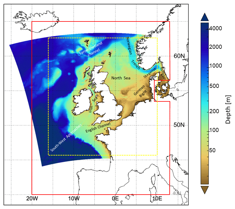
Figure 1European Marine Observation and Data Network (EMODnet bathymetry, in metres (logarithmic scale), showing the NWS high-resolution AMM15 model domain. The red line defines the NWS low-resolution AMM7 model domain. The yellow dotted box is the domain covered by the AMM15 products delivered on a regular grid to the Copernicus users. Figure is modified from Graham et al. (2018b). The bathymetry colour range has a logarithmic scale.
There is therefore a significant history of marine monitoring and prediction in support of sustainable use of our marine environment, with the safety of life at sea imperative, leading to surface wave models providing forecasts, followed by ocean model forecasts predominantly by the need for storm surge prediction and (more recently) currents and hydrodynamics, mainly led by defence requirements, but also supporting industry and marine planning (Siddorn et al., 2016). Most recently of all, there has been an increasing focus on sustained monitoring and forecasting of the lower trophic ecosystem and marine biogeochemistry (She et al., 2016). The Met Office, with the support of collaborators from around the NWS region, has been producing freely available marine predictions and forecasts for this region for a number of years as part of the Copernicus Marine Environment Monitoring Service (CMEMS; Le Traon et al., 2017; Tonani et al., 2017) and precursor projects (e.g. Siddorn et al., 2007; O'Dea et al., 2012).
The operational ocean forecasting systems developed with the Forecasting Ocean Assimilation Models (FOAM) are based on a seamless prediction philosophy whereby the global and regional systems rely on similar ocean modelling and assimilation tools, and are co-developed for short-range forecasting, seasonal forecasting (e.g. MacLachlan et al., 2015; Tinker et al., 2018), and climate predictions (Williams et al., 2018). The operational forecasting configuration for the NWS is a FOAM system designed to deal with the specific constraints of operational oceanography on a shallow continental shelf sea. The model domain (shown in Fig. 1) extends into the Atlantic Ocean to resolve exchanges across the shelf, of primary importance for the continental shelf seas' dynamics and water properties. The Atlantic region is chosen to allow the propagation and downscaling onto the shelf of phenomena associated with the large-scale open ocean circulation. For example, the North Atlantic Current and European Slope Current which transport heat and salt from the north-east Atlantic, interact with the continental shelf slope and form branches that flow into the North Sea. The boundaries in the Baltic cover the Kattegat–Skagerrak area, to provide the Baltic inflow, which has a significant influence on the region's water masses due to the significant, and highly variable, freshwater fluxes.
The NWS system has three major components: an ocean model coupled with a biogeochemistry model and a variational data assimilation scheme. This system runs a forecast cycle every day to provide 6 d forecasts of the physical and biogeochemical variables in this area. The forecast is initialized by running two 24 h analysis cycles. By assimilating observations in this way, the FOAM system incorporates information from considerably more observations than would be available in near-real time with a single 24 h window, due to the addition of late-arriving observations.
Until recently, the operational system for this region has been run at approximately 7 km horizontal resolution (O'Dea et al., 2012; King et al., 2018). This paper describes the operational implementation of the 1.5 km version of this ocean model, referred to as the Atlantic Margin Model, or AMM15 (Graham et al., 2018a). The dominant dynamical scales decrease with reducing water depth and have complex interactions with tidal phenomena and other bathymetric interactions requiring a modelling system at a kilometric scale resolution for this region (Polton, 2014; Holt et al., 2017). The increase of resolution to 1.5 km is therefore a fundamental step change in the ability to resolve key processes and features in the NWS region (Guihou et al., 2017). As well as being developed for ocean forecasting operations, the AMM15 is being used within a coupled ocean–wave–atmosphere research system (Lewis et al., 2019a, b).
The upgrade of the NWS system to AMM15 does not yet include the biogeochemical component as the computational cost is prohibitive, with the production time exceeding the 24 h for a full hindcast–forecast cycle. Two systems are therefore being run in parallel: (i) the 7 km AMM7 model with the physical and biogeochemical components similar to O'Dea et al. (2012) and (ii) a 1.5 km AMM15 physics only system (being detailed in this paper), as described in Fig. 2. An AMM15-based coupled physics–biogeochemistry model is under development, and techniques are being developed to reduce the computational cost to allow it to be implemented within the time constraints of operational production. Herein, we describe only the physical component of the high-resolution system (AMM15), highlighting the differences with the low-resolution configuration (AMM7). O'Dea et al. (2012, 2017) provide full descriptions of the AMM7 version of this system. It is worth noting here that the NWS system also has a wave component providing products on the same grid as the AMM15 (Fig. 2). The wave and physical models are forced by the same wind fields, and the wave model uses the surface currents computed by AMM15. However, the wave model description and validation are not within the scope of this paper.
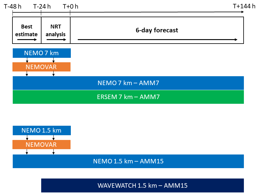
Figure 2FOAM daily production cycle. The 7 km system, top panel, has an ocean model coupled with a biogeochemical model and a variational assimilation scheme. The 1.5 km system, bottom panel, has an ocean model with a variational assimilation scheme and a wave model, forced by the ocean model surface currents (not coupled).
The 7 km products (AMM7) delivered through Copernicus are
-
NORTHWESTSHELF_ANALYSIS_FORECAST_ PHYS_004_001_b (http://marine.copernicus.eu/documents/PUM/CMEMS-NWS-PUM-004-001.pdf, last access: 15 August 2019);
-
NORTHWESTSHELF_ANALYSIS_FORECAST_ BIO_004_002_b (http://marine.copernicus.eu/documents/PUM/CMEMS-NWS-PUM-004-002.pdf, last access: 15 August 2019).
The 1.5 km products (AMM15) delivered though Copernicus are
-
NORTHWESTSHELF_ANALYSIS_FORECAST_ PHY_004_013 (http://marine.copernicus.eu/documents/PUM/CMEMS-NWS-PUM-004-013.pdf, last access: 15 August 2019);
-
NORTHWESTSHELF_ANALYSIS_FORECAST_ WAV_004_014 (http://marine.copernicus.eu/documents/PUM/CMEMS-NWS-PUM-004-014.pdf, last access: 15 August 2019).
This study is focused on the NORTHWESTSHELF_ANALYSIS_FORECAST_PHY_004_013 product and its intercomparison with NORTHWESTSHELF_ANALYSIS_FORECAST_PHYS_004_001b.
Here, we provide details on the AMM15 hydrodynamic model, the data assimilation scheme, and the operational suite in the following section. Section 3 will then describe the trial experiments, while Sect. 4 details our assessment of the new high-resolution products. Our conclusions are presented in Sect. 5.
2.1 Core model description
The FOAM 1.5 km AMM15 is a hydrodynamic model, one-way nested within the Met Office operational North Atlantic 1∕12∘ deep ocean model (Storkey et al., 2010) and the CMEMS operational Baltic Sea model (Berg and Weismann Poulsen, 2012). The model core is based on version 3.6 of the Nucleus for European Modelling for the Ocean (NEMO; Madec and the NEMO Team, 2016). This is a community ocean modelling system that has a wide user and developer base, particularly in Europe.
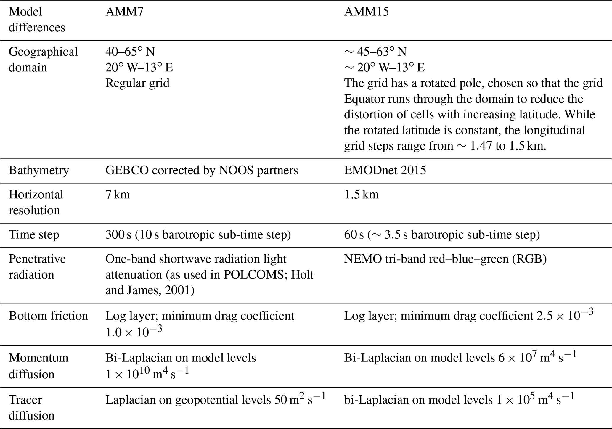
The regional model is located on the NWS, extending from approximately 45 to 63∘ N and from 20∘ W to 11∘ E. There is a uniform grid spacing of ∼1.5 km throughout, in both the zonal and meridional directions (Graham et al., 2018a). The vertical coordinate system is based on a hybrid s-sigma terrain-following system, (Siddorn and Furner, 2013), with 51 vertical levels. This is the same as that used in AMM7, with the thickness of the surface cell set to ≤1 m to guarantee uniform surface heat fluxes across the domain. The terrain-following coordinates used here are fitted to a smooth envelope bathymetry, where the level of smoothing is determined such that the local bathymetric slope , computed between adjacent bathymetry points hi and hi+1, is constrained to be less than a specified maximum value (rmax). This is required to mitigate against spurious horizontal velocities that arise from horizontal pressure gradient errors in terrain-following coordinates that are too steep. Although the number of levels in both AMM15 and AMM7 is the same, the steeper gradients resolved in AMM15 mean that a lower rmax value was chosen (0.1, compared to 0.24) to ensure stability along the shelf break.
The bathymetry chosen for AMM15 (and shown in Fig. 1 and summarized in Table 1) is from the European Marine Observation and Data Network (EMODnet portal, September 2015 release). The increased resolution of both AMM15 and this EMODnet data set allows for improved representation of fine-scale features and processes, particularly along the shelf break. The original EMODnet data are referenced to lowest astronomical tide (LAT) and thus have been converted to mean sea level (MSL) for use in the model. The differences between LAT and MSL referenced bathymetry are negligible in the deep ocean but can be large on-shelf, particularly in shallow coastal areas with large tidal ranges. The model minimum depth is forced to be 10 m, due to the tidal limit and lack of wetting and drying. This choice ensures that no locations dry out, due to the tides. Further details on the model domain and bathymetry can be found in Graham et al. (2018a).
Tidal modelling requires a non-linear free surface, and this is facilitated in NEMO by using a variable volume layer method. The short timescales associated with tidal propagation and the free surface require a time-splitting approach, splitting modes into barotropic and baroclinic components. The model uses a non-linear free surface, an energy- and enstrophy-conserving form of the momentum advection, and a free-slip lateral momentum boundary condition. The tracer equations use a TVD (total-variance-diminishing) advection scheme (Zalesak, 1979).
Since both AMM15 and AMM7 have a similar vertical grid, the vertical parameterizations remain similar. The generic length-scale scheme is used to calculate turbulent viscosities and diffusivities (Umlauf and Burchard, 2003). Dissipation under stable stratification is limited using the Galperin limit of 0.267 (Holt and Umlauf, 2008). Bottom friction is controlled through a non-linear log layer, with a minimum drag coefficient of (compared with a coefficient of in AMM7), as described in Table 1.
As many more fine-scale mixing processes are resolved in AMM15, only minimal eddy viscosity is applied in the lateral diffusion scheme. For momentum and tracers, bi-Laplacian viscosity is applied on model levels with coefficients of 6×10⁷ and 1×10⁵ m4 s−1, respectively. For AMM7, additional viscosity and eddy diffusivity must be parameterized. A bi-Laplacian scheme is used on model levels for momentum, with a coefficient of 1×10¹⁰ m4 s−1. For tracer diffusion, a Laplacian diffusion scheme is used on geopotential surfaces, with a coefficient of 50 m2 s−1 (Table 1).
Boundary and surface forcing
Tidal forcing is included both on the open boundary conditions via a Flather radiation boundary conditions (Flather, 1976) and through the inclusion of equilibrium tide. The TOPEX/Poseidon cross-over solution (Egbert and Erofeeva, 2002; TPX07.2, Atlantic Ocean 2011-ATLAS) provides 11 constituents for amplitude and phase of surface height and velocity at 1∕12∘.
The model is one-way nested with the Met Office operational North Atlantic 1∕12∘ deep ocean model (Storkey et al., 2010) and the CMEMS operational Baltic Sea model (Berg and Weisman Poulsen, 2012). They provide temperature, salinity, sea surface height (not at the Baltic boundary), and depth-integrated currents at the open boundaries. The two models, AMM7 and AMM15, are both nested in the open Atlantic and Baltic boundaries to the same products, but the boundaries are in a different geographical position due to the different model domains.
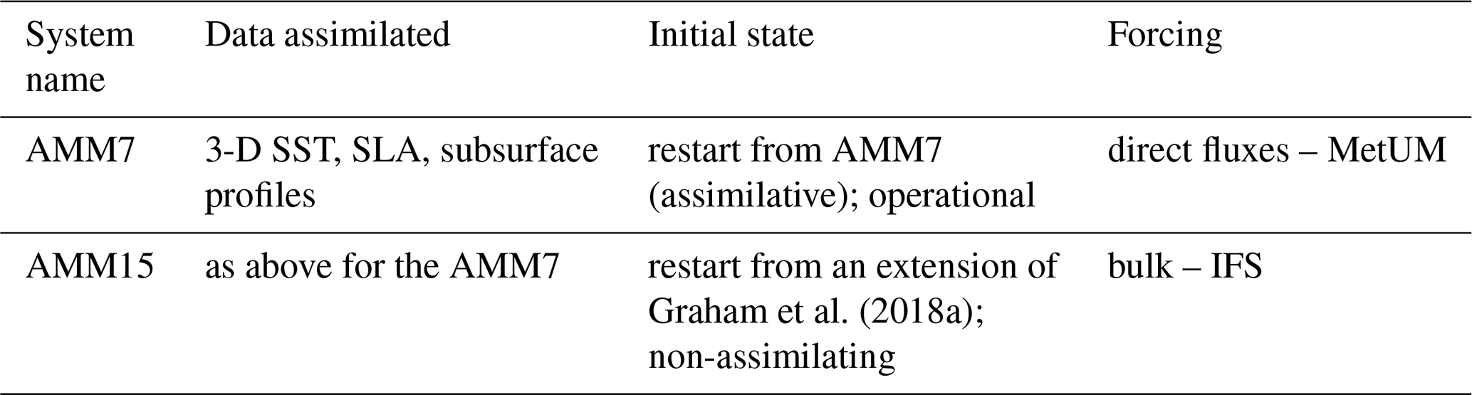
AMM7 and AMM15 are forced at the air–sea interface by two different numerical weather prediction (NWP) outputs, the Met Office Unified Model (MetUM) global atmospheric model for AMM7 and the European Centre for Medium-Range Weather Forecasts (ECMWF) operational Integrated Forecasting System (IFS) for AMM15; see Table 2 for details. The Copernicus Marine Environment Monitoring Service requested the change from the MetUM to IFS forcing with the aim of minimizing differences among the regional systems covering all the European seas. The fields from ECMWF and Met Office have a similar spatial resolution, but IFS fields for wind and atmospheric pressure have a lower temporal resolution as described in Table 2. The IFS analysis is available only at a low temporal resolution (6 h); therefore, the decision was made to force the system using forecast fields only (3 hourly) from the 00:00 UTC forecast base time run. A specific set of experiments is needed to assess the impact of this choice but are not within the scope of this paper. ECMWF products at higher temporal resolution are now available and will be used in future releases of this operational system, improving the atmospheric forcing of this first version of AMM15. The IFS forcing is applied using the Common Ocean-ice Reference Experiment (CORE) bulk formulae (Large and Yeager, 2009). The specific humidity, sH, not available from the IFS field, is computed from the dew point temperature at 2 m and the surface pressure using the World Meteorological Organization formulation (WMO, 2010):
where mwa is the ratio between the molecular weight of water and of dry air; rSP is the reference surface pressure; SP is the surface pressure. The AMM7 instead is forced at the surface by direct fluxes from MetUM and using the Coupled Ocean-Atmosphere Response Experiment (COARE4) bulk formulae, as described in O'Dea et al. (2012).

An atmospheric pressure gradient force is applied at the surface of both models, using the atmospheric pressure field from MetUM and IFS, respectively, which affects the model free surface elevation.
The light attenuation in AMM15 is set to the standard NEMO tri-band scheme (RGB), assuming a constant chlorophyll concentration (Graham et al., 2018a). AMM7 uses the single-band light scheme previously used in the Proudman Oceanographic Laboratory Coastal Ocean Modelling System (POLCOMS) and outlined in Holt and James (2001). In this single-band light scheme, the extinction depths vary across the domain in proportion to the bathymetry in order to estimate the change in water clarity between deep and shallow waters.
For AMM15, river runoff is based predominantly on a daily climatology of gauge data averaged for 1980–2014. UK data were processed from raw data provided by the Environment Agency, the Scottish Environment Protection Agency, the Rivers Agency (Northern Ireland), and the National River Flow Archive (gauge data were provided by Sonja M. van Leeuwen, CEFAS, Lowestoft, UK, personal communication, 2016). For major rivers that were missing from this data set (e.g. along the French and Norwegian coasts), data have been provided from an earlier climatology (Young and Holt, 2007; Vörösmarty et al., 2000), based on a daily climatology of gauge data averaged for the period 1950–2005, which is the climatology used by AMM7. The differences between AMM15 and AMM7 river discharge data are expected to be mainly, but not only, along the UK coastline.
2.2 Assimilation method
The data assimilation component of FOAM is NEMOVAR, a multivariate, multi-length-scale assimilation scheme developed collaboratively by the Met Office, the Centre Européen de Recherche et de formation avancée en calcul scientifique, the ECWMF, and the Institut National de Recherche en Informatique et en Automatique (Mogensen et al., 2012). This has been implemented at the Met Office as an incremental 3D-Var, first guess at appropriate time (FGAT) scheme for the 1∕4∘ global model (Waters et al., 2015) and the AMM7 (King et al., 2018).
An assimilation window of 24 h is used, and observations assimilated include in situ and satellite-swath sea surface temperature (SST) observations, altimeter measurements of sea level anomaly (SLA) (in regions with depth > 70 m), and profile observations of the subsurface temperature and salinity from a number of sources as detailed in Table 3. The SLA observations assimilated in this model are provided through CMEMS and include the corrections necessary to add back the signals due to tides and wind and pressure effects necessary for use with a wind- and pressure-forced tidal coastal model (King et al., 2018). After the assimilation step, the model is re-run for the same period with a fraction of the increments applied to the model fields at each time step – the incremental analysis update procedure (Bloom et al., 1996).
Table 3List of observations used for data assimilation.
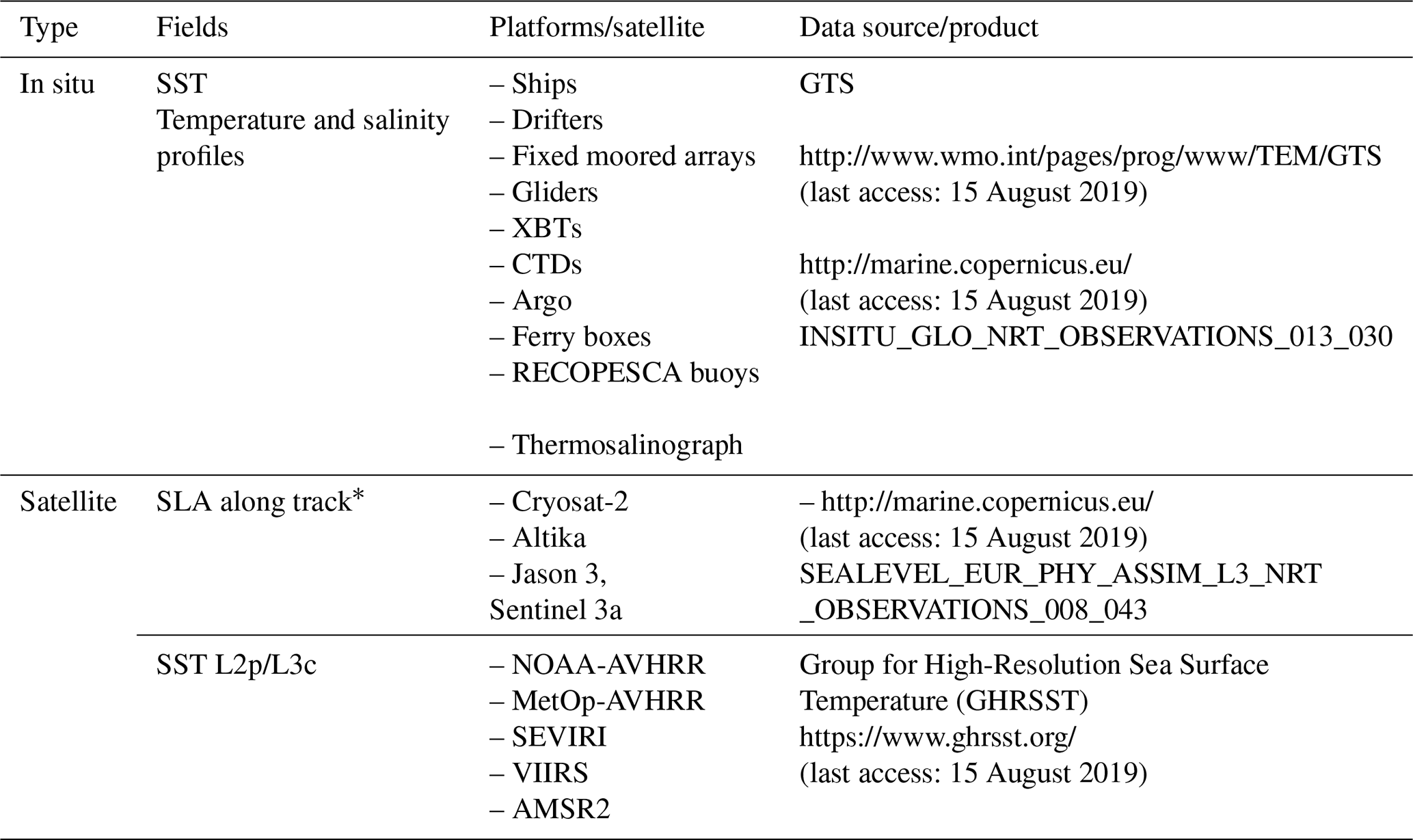
* Along with the corrections necessary for the use with a wind- and pressure-forced tidal coastal model. SLAs are assimilated only in deep regions (>700 m).
The Met Office implementation of NEMOVAR includes bias correction scheme for both SST and altimeter data. The SST bias correction aims to correct for biases in the observed SST due to the synoptic-scale atmospheric errors in the satellite retrievals, while for SLA we apply a slowly evolving bias correction to correct for errors in the mean dynamic topography (MDT) (Lea et al., 2008).
In the AMM15 implementation described here, the assimilation component has been upgraded to NEMOVARv4, which introduced a small number of changes compared to the scheme used in AMM7 (detailed in Table 4). In the AMM7 configuration, which uses NEMOVARv3, the SST bias correction scheme employs observations of bias (determined by matching nearby, contemporaneous in situ and satellite observations) to estimate a daily correction to the observations from each SST satellite. In NEMOVARv4, a variational bias correction has been introduced which combines information from average SST innovations with the observations of bias used previously. We have also included observations from the Visible Infrared Imaging Radiometer Suite (VIIRS) in our reference data set against which the other satellite SST observations are bias corrected. This new scheme has been shown to be more resilient to changes in the observing system and gaps in observation coverage (While and Martin, 2019). The SLA bias correction in AMM15 is unchanged from AMM7.
Table 4AMM15–AMM7 differences in the data assimilation scheme.
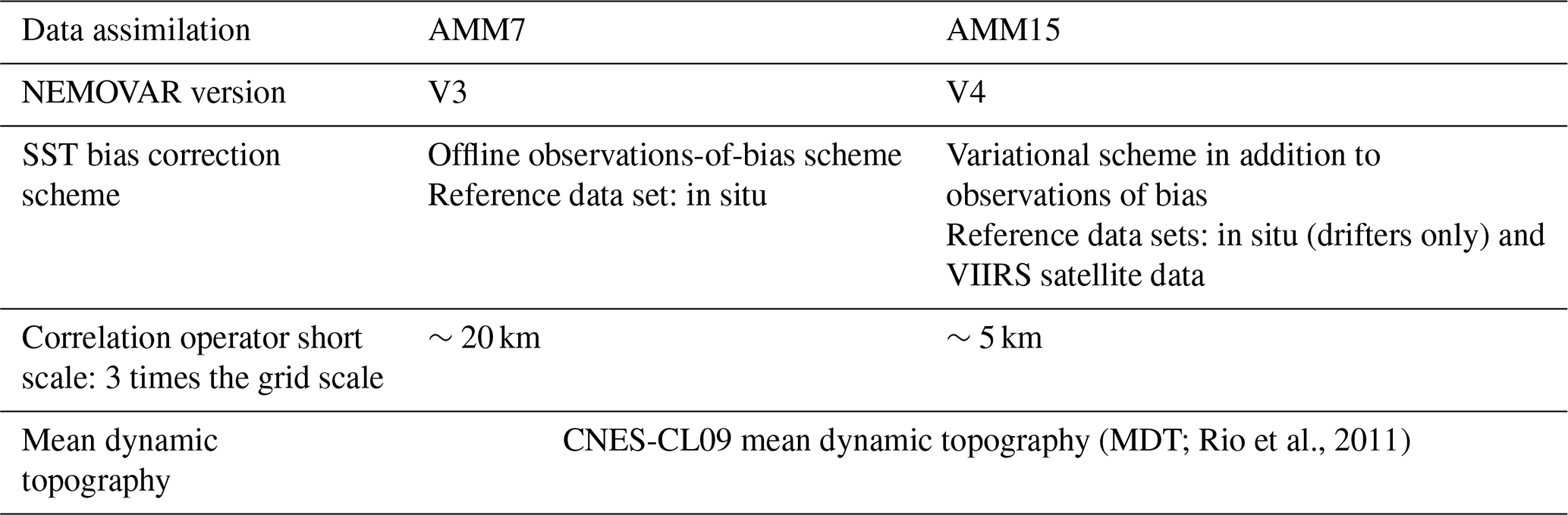
Although the same observation and background error variances are used in AMM15 as in AMM7 (see King et al., 2018), the background error correlation length scales have been modified. The spatial covariance of background errors is modelled using an implicit diffusion operator with the horizontal length scales specified a priori, and the vertical length scales specified using a parameterization based on the mixed layer depth. In NEMOVARv3, this was modelled using three 1-D diffusion operators, but in NEMOVARv4 it is modelled using a 2-D horizontal diffusion with a 1-D vertical diffusion (Weaver et al., 2016). In both systems, two horizontal correlation length scales are used (Mirouze et al., 2016): 100 km for the long length scale and the Rossby radius of deformation for the short length scale. To avoid numerical computation issues, the short length scale is restricted to have a minimum value equivalent to 3 times the grid scale. This has the result that in shallow water the short length scale for AMM15 can be as small as 4.5 km compared to 21 km for AMM7.
2.3 Operational production
The FOAM system produces daily 2 d analyses (best estimate and near-real-time – NRT – analysis) and a 6 d forecast (Fig. 2). The timeliness of the observations, in situ and from satellite, significantly affects the number and the quality of the observations available in the 24 h preceding the forecast, so two analysis cycles of 24 h each are run to include as many observations as possible in the data assimilation.
The observations are downloaded from different sources: CMEMS for sea level anomaly L3 products, Group for High Resolution Sea Surface Temperature for the L2 SST satellite observations and the Global Telecommunication System (GTS) and CMEMS for the in situ observations. The vertical profiles need to be thinned to reduce the spatial error correlation between the observations. For a given 24 h, they are thinned in 3-D space with the values: Δlong, Δlat = 0.2∘, Δz=10 m. Prior to data assimilation, a quality check of the observation is performed using the model background produced by the forecast cycle of the previous day (Ingleby and Huddlestone, 2007). Observations flagged as bad are not used for the data assimilation. The quality check for the vertical profiles is performed at 51 geopotential standard depth. The full profile is rejected only if more than one-half is flagged as bad. The quality-control (QC) information, the background and observations fields are stored in specific files, known as feedback files. The error thresholds for the QC are set in order to avoid unrealistic model fields due to bad observations.
The lateral boundaries for the Atlantic region and the Baltic are both from the forecast production of the previous day. The Baltic boundaries are downloaded every morning a few hours before starting the operational suite for the NWS. The CMEMS Baltic Sea product has 5 d forecast, produced twice a day, at 00:00 and 12:00 UTC, and delivered at 07:00 and 19:00 UTC, respectively. The NWS models are forced with the latest data available at 05:00 UTC and the last hourly field is persisted to produce the last day of forecast.
The atmospheric forcing is downloaded from ECMWF and since the last set of data is available at 07:00 UTC, production is started 15 min later to allow for download delays. Once the model and data assimilation task are over, the post-processing task starts because the products need to be organized for delivery to the users. The raw output files are interpolated on a standard grid at the same resolution as the model-rotated grid (1.5 km) but covering a slightly smaller area (see the yellow rectangular dotted line in Fig. 1). The vertical terrain-following levels are converted for users' convenience into 33 standard geopotential levels: (surface, 3, 5, 10, 15, 20, 25, 30, 40, 50, 60, 75, 100, 125, 150, 175, 200, 225, 250, 300, 350, 400, 450, 500, 550, 600, 750, 1000, 1500, 2000, 3000, 4000, and 5000 m). All the files are then packaged to be compliant with the CMEMS and CF standards. Each day, the best estimate (T−48 h, T−24 h) and NRT (T−24 h, T+00 h) analyses are delivered as well as 6 forecast days for all products (with the first day of the forecast being for the day of production). The delivered products are 25 h daily means and hourly instantaneous products of temperature, salinity, horizontal currents, sea surface height (SSH), and mixed layer depth (MLD). Daily mean values are calculated as means of 25 instantaneous hourly values, starting at midnight and finishing on the following midnight to remove the tidal cycles. The data are in NetCDF4 format and the volume of each production cycle is ∼14 GB (1.7 GB for each day), while for AMM7 it is ∼1 GB.
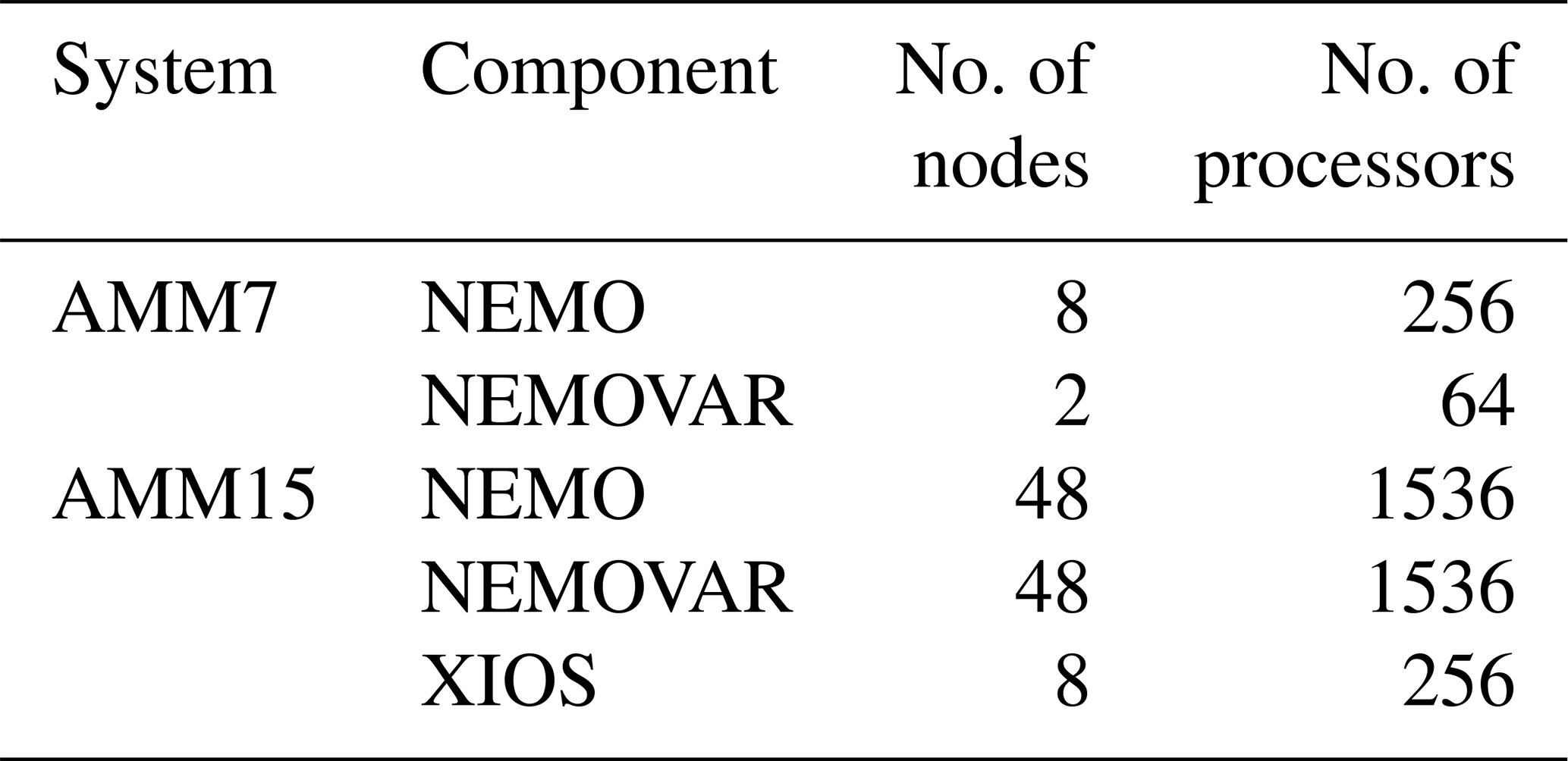
AMM15 is running on the Met Office high-performance computing (HPC) Cray XC40 super computer using 48 nodes and 1536 processors. AMM7 instead is using only 8 nodes and 256 processors. This information is summarized in Table 5 for each component of the system: XIOS is for the I/O of NEMO. The small size of AMM7 model grid does not require dedicated nodes for this task.
Table 5AMM7 and AMM15 computational resources on the Met Office HPC Cray XC40.
The production process takes approximately 4 h, which is 4 times that required by AMM7. It is planned to improve the robustness of this first implementation of the system by improving the dependencies of the different tasks in the operational suite and investigating ways of reducing the dependency on IFS delivery. The quality of the products and the observations used for the production is monitored each day to allow the ocean forecasting scientists to take action if there are anomalies in the production or missing observations, and to allow users to be promptly alerted in the case of degradation of the products.
The assessment of the pre-operational implementation is based on trial experiments covering the years 2016–2017 (Table 6). The strategy for trialling forecasting systems prior to entering into operations is one of significant debates at the time of writing. Ideally, given the relatively poor in situ observational coverage, a long period of trialling would be used to assess the system performance to gain a full (and statistically significant) understanding of its performance in all seasons and under a range of conditions. However, a combination of the length of time and computational cost to run those trials, the overhead in preparing observations and fluxes, and the difficulty in finding a period of observations and fluxes that truly reflect the operational conditions led to a more pragmatic approach being taken. It should be noted that the AMM15 modelling system itself has already been assessed for a long period and its quality documented in Graham et al. (2018a). Similarly, the data assimilation methodologies are well-tested (King et al., 2018) and have been robust in operations in other implementations. This assessment is therefore complementary and allows an assessment of the system as it is in operations, with fluxes, boundaries, and assimilated observations used that are similar to the operational system. The trial experiments are required to cover a period in the recent past in order to avoid differences in the observational network and/or in the forcing resolution/quality. The 2 years that were chosen are therefore a balance between covering a multi-year period that is recent in time (and hence representative of the operational conditions) and achievable on the timescales required to transition into operations.
Before adding a new product to the operational production, the system must be shown to offer an improvement over the previous system. For AMM15, this was done by setting up comparative trials running the existing and the new system, which are running with different forcing and initial conditions. This assures that we reproduce the operational products, new and old, and we validate the quality of the products.
The operational version of AMM7 was re-run rather than using the operational products produced in real time in order to avoid inconsistency in the number and type of observations assimilated by the two systems. Indeed, the real-time production can suffer temporary delays or problems in the delivery of the observations that are not reproducible in delayed time.
A free (non-assimilative) run was performed as a control, for both AMM7 and AMM15, but the results are not described in this work, since our aim is to assess the quality of the products delivered to the users. Apart from the resolution, the major differences between AMM7 and AMM15 are in the initial conditions, the atmospheric forcing, and the location of the lateral boundaries.
The AMM7 initial conditions are from the operational (assimilating) system, while for AMM15 they are from an extension of the non-assimilating experiments presented in Graham et al. (2018a), which finished at the end of 2014. This run was extended to include 2015 and was run with the same source of atmospheric forcing and Atlantic lateral boundary used for 2016–2017. However, the CMEMS Baltic data sets used to calculate the boundaries used in operations for AMM7 are no longer available due to the CMEMS retention policy and thus cannot be used to calculate the AMM15 equivalents. We therefore used the CMEMS product where it was available (for the years 2016 and 2017), but for 2015 a general estuary transport model (GETM; Burchard and Bolding, 2002) implementation for the Baltic (as used by Graham et al., 2018a) was used in its place.
This paper details the assessment of the quality of the AMM15 operational system based on the assimilative run and is therefore representative of the analysis day. Graham et al. (2018a) have demonstrated that the AMM15 without data assimilation performs equally as well as or better than AMM7. A detailed assessment of the forecast based on the real-time forecast produced since the beginning of November 2018 will be conducted in the future. It is anticipated that the forecast quality improvement for the AMM15 against the AMM7 will be greater than the improvement for the analysis day, given the improved underlying model, but that must still be demonstrated.
The results and validation of these trials are used for two purposes: as a basis for making a decision on whether to proceed with the operational implementation, and to provide feedback to the researchers developing the models and data assimilation systems to prioritize their research activities.
The observations assimilated in the NWS system are SST from in situ and satellite, SLA from satellite, and subsurface vertical profiles, as detailed in Table 3. The satellite measurements guarantee a good coverage of the area, especially for SST, while the subsurface profiles are variable in terms of number of observations and spatial/geographical distribution. Figure 4 shows the observations distribution during the years 2016–2017 for subsurface observations of temperature and salinity for the two most extreme seasons in terms of data distribution, winter (defined as December–January–February) and summer (June–July–August). In the summers of 2016 and 2017, there were very few observations on-shelf, in particular in the North Sea, and this had an impact on the quality of the assimilative runs. Compared to the trial experiments, done in delayed time, the real-time analysis can have a temporary decrease of quality due to timeliness issues affecting the real-time delivery of observations or poor quality-controlled data.
3.1 System performance: AMM15 vs. AMM7
The impact of the high resolution can be qualitatively assessed comparing models' surface current maps. The current field of AMM15 is more detailed and seems more realistic than AMM7 but the lack of the observations makes it difficult to properly assess the horizontal velocity field in key areas. Figure 3 represents the surface currents from AMM7 and AMM15 for a single day to give an example of the difference between the two models. AMM15 has a more complex current circulation in the deep part of the shelf, with meanders and eddies, not resolved by AMM7. The European slope current, green arrow in Fig. 3, is transporting Atlantic water into the North Sea, mainly through the Faroe–Shetland Channel (Marsh at al., 2017), influencing the characteristic of the water in the northern North Sea and its circulation. The AMM15 current patterns seems more realistic, reproducing eddies and meanders, as shown by drifter measurements done in this area (Burrows and Thorpe, 1999). The European slope current plays a major role in the across-shelf transport, with AMM15 better reproducing the water exchanges as described in Graham et al. (20018b).
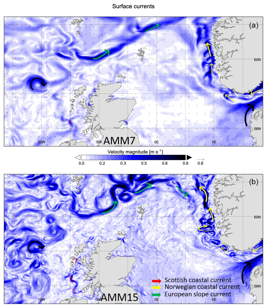
Figure 3Surface current from AMM7 (a) and AMM15 (b) (daily mean of 2 December 2018).
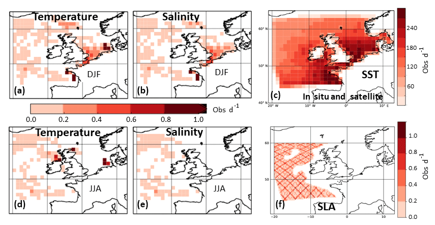
Figure 4Number of observations per day for various observation types over 2016/2017: winter (DJF) temperature (a) and salinity (b) profiles in 2∘ bins, summer (JJA) temperature (d) and salinity (e) profiles, in situ and satellite SST (c), and satellite SLA (f).
The two models are also very different in the area characterized by the Norwegian Coastal Current (NCC) which is highlighted by the yellow vectors in Fig. 3.
The NCC is a coastal current flowing from Skagerrak to the Barents Sea, following the Norwegian coastline, in the upper layer (50–100 m) over the Norwegian Trench. This current is characterized by a front between low-salinity water coming from the brackish Baltic Sea and Norwegian coastal water, and the Atlantic water. This current has mesoscale meanders and eddies (Ikeda et al., 1989) propagating northward along the Norwegian coast. AMM15 reproduces better the mesoscale eddies and meanders of the NCC which are not resolved by AMM7.
The Scottish coastal current seems to be well resolved by AMM15, with a strong current flowing along the west Scottish coast and meandering before entering the channel between mainland Scotland and the Hebrides (the Minch). This is a persistent current that interacts with the island chain of the Hebrides (Simpson and Hill, 1986). AMM15 has a more detailed coastline and bathymetry in this area which is likely to be one of the main reasons why the model resolves this current. In AMM7, this current is almost absent, or too weak and misplaced to the west, instead of being, as it in AMM15, between the islands and the mainland (Fig. 3, red arrows). The contrast between the low salinity along the coast and the higher salinity of the Atlantic water is another key driver of this current (Simpson and Hill, 1986), and this is better represented by AMM15, which has an improved salinity field compared to AMM7 (see Sect. 4). AMM15 seems to be much less diffusive in the proximity of the river plumes keeping a narrower plume close to the coast and has a lower lateral diffusion (Graham et al., 2018a). AMM7 has low-salinity water (less than 34.5 psu) spreading much further away from the coast, all the way to the Outer Hebrides, while the salinity gradient in AMM15 is located between the Minch and the western side of the Outer Hebrides. This assessment shows that AMM15 is in very good agreement with literature in this area. Further studies, and possibly targeted observations, are needed to validate this preliminary result and to assess AMM15 skills in predicting the seasonal variability of this current and the other currents described in this study.
Most of the observations used for the global validation are the same as used for the data assimilation, as described in the previous section. The model–observation differences are calculated before the model is corrected by the assimilation, but even so the observations are not fully independent from previously assimilated observations. All the same, this method is commonly used for model validation (King et al., 2018) and we consider the validation significant. Independent observations, available on a very limited geographical domain and/or for a shorter period than the 2 years, have also been used, and have the benefit of providing an understanding of the impact of the high resolution locally on small areas and short timescales. This approach differs from the validation described in Graham et al. (2018a), which focussed on the seasonal, interannual, and multi-year timescales.
The independent observations we have used are
-
glider transects from the UK MASSMO4 experiments (north of Scotland),
-
the Coastal Observing System for Northern and Arctic Seas (COSYNA) high-frequency (HF) radar in the German Bight,
-
tide gauges, and
-
moorings in the German Bight and in the English Channel.
The geographical location of these observations is presented in Fig. 5 where each type of observation is marked by a different colour. Also used was the Operational Sea Surface Temperature and Sea Ice Analysis (OSTIA) L4 SST product (Donlon et al., 2012) which, although not assimilated, is not fully independent as it assimilates a similar (but not identical) set of SST observations to the AMM7 and AMM15 using similar methods (including using the same assimilation framework, albeit set up slightly differently).
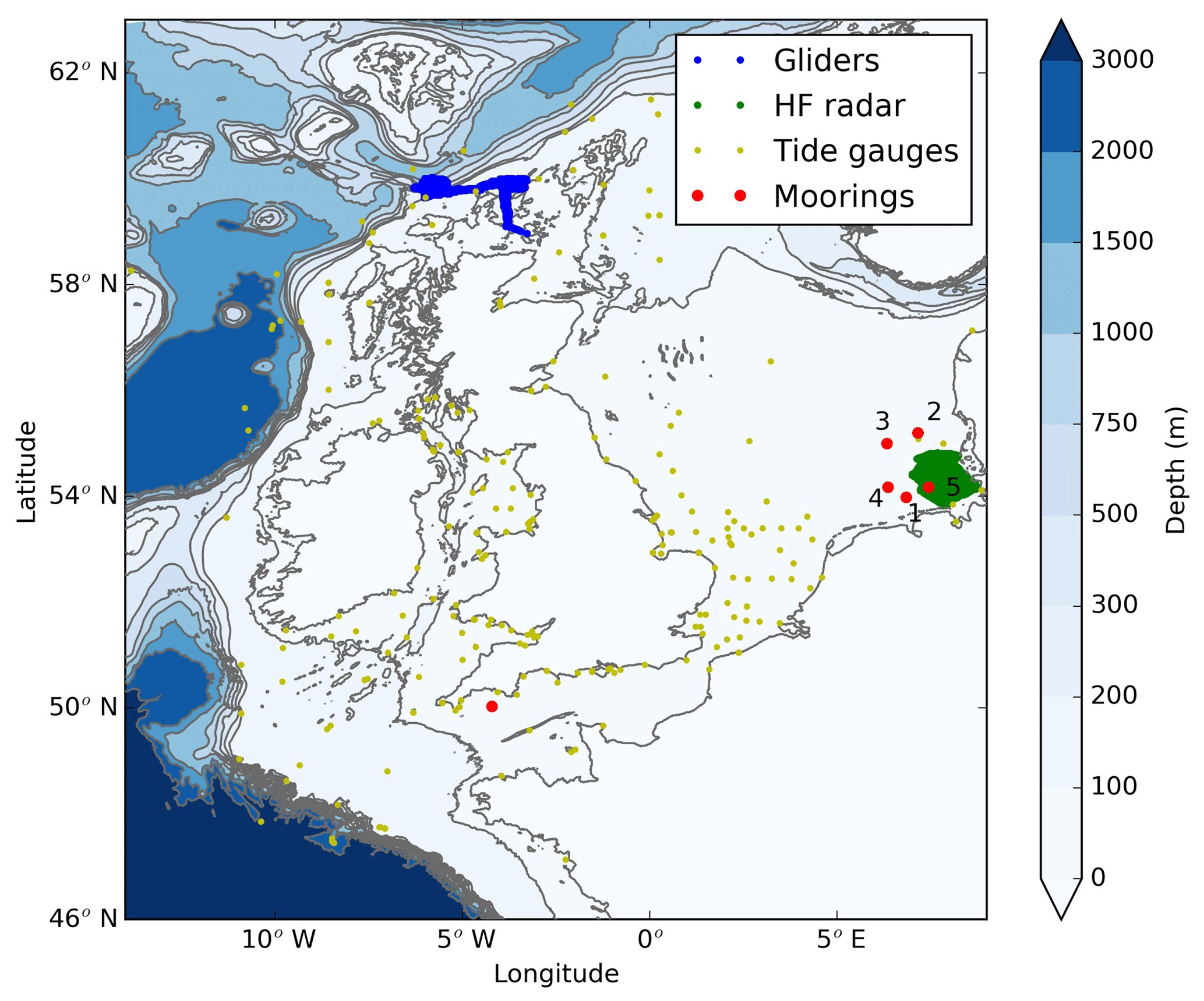
Figure 5Maps of the independent observations used for validation. MASSMO4 gliders are blue, COSYNA HF radar in the German Bight in green, the mooring in the German Bight in red, and the tide gauges in yellow.
The basin-scale validation results for AMM7 and AMM15 are summarized in Table 7 (with the system that has the best quality highlighted in bold), with a short description of the observations used. The ambition is to validate all the variables delivered to the users, even if there is a huge difference in the number and quality of observations available for the different parameters.
Table 7Synthesis of the validation results for AMM7 and AMM15. The values in bold indicate an improvement.
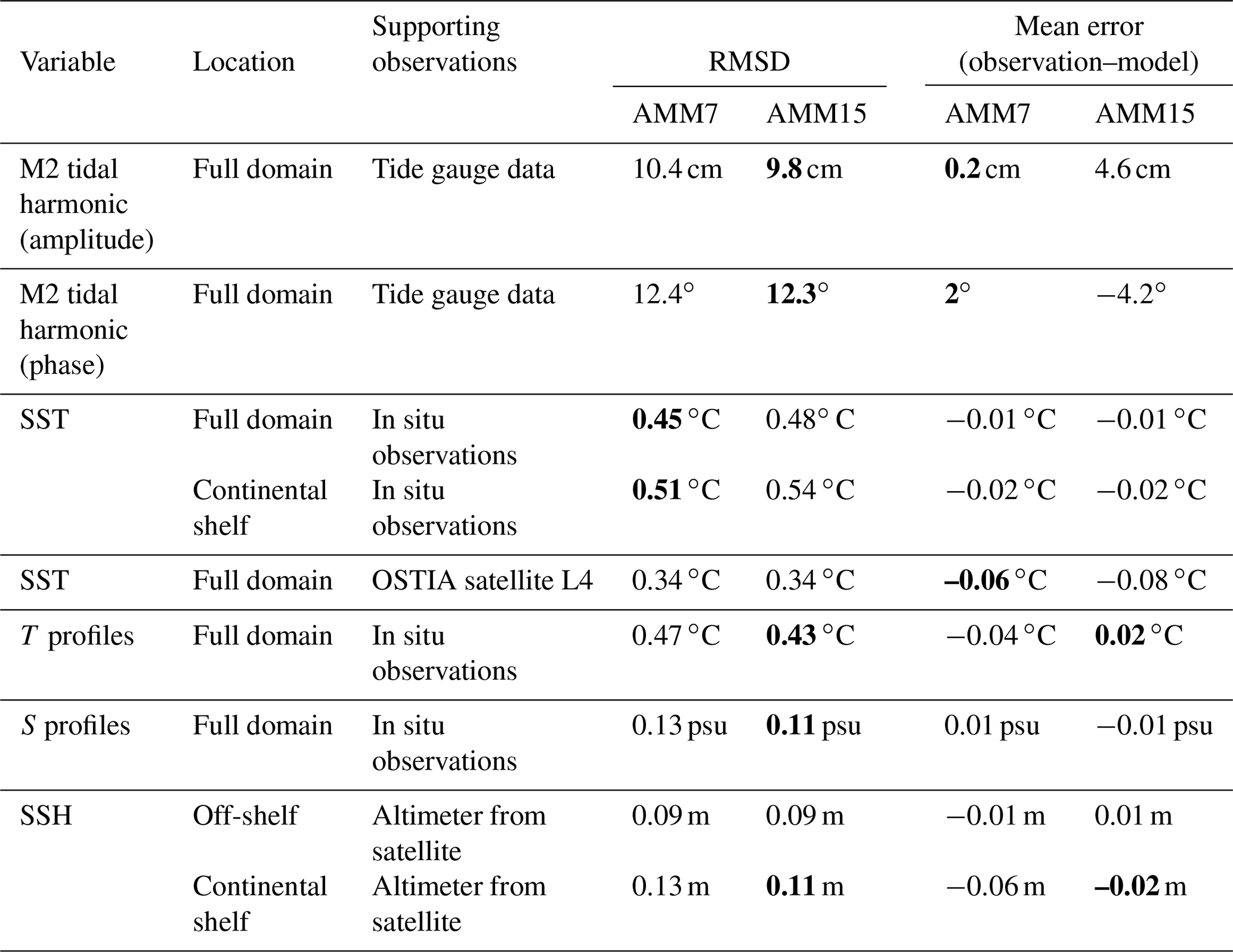
The root mean square difference (RMSD) and mean error (or bias) values are similar between the two systems and do not reflect the AMM15 system's superior performance as the validation at basin scale, averaged over the whole 2-year or 1-year period, penalizes the high-resolution system. Whilst higher-resolution models (subjectively) generate more realistic fields, it is often the case that statistics based on direct point matchup between interpolated model and observations do not improve due to the double penalty effect (e.g. Brassington, 2017). So, although global statistics do not show significant improvement from AMM7 to AMM15, it is demonstrated below that AMM15 consistently performs better than AMM7 when validated locally against high-resolution observations. It is an active area of research both with the ocean and numerical weather prediction communities to understand how to quantitatively demonstrate skill improvement from higher-resolution systems, and something that needs a real focus from our community.
4.1 Tides
Most of the continental shelf seas' dynamics is dominated by tidal variability, which impacts the velocity fields and plays a key role in the mixing and the generation of fronts. The improved resolution per se does not imply an improvement in capability to model the tidal signal even if differences in the topography and coastlines could affect the baroclinic component of the tide influenced by interaction of the flow with the bathymetry. This is particularly true in shallow areas when tidal currents are strong. We have assessed the tides for the years 2016 and 2017 using the tidal gauges. In addition, we used HF radar velocity data available in a small part of the domain, in the German Bight (south-east North Sea), for a single month (March 2017).
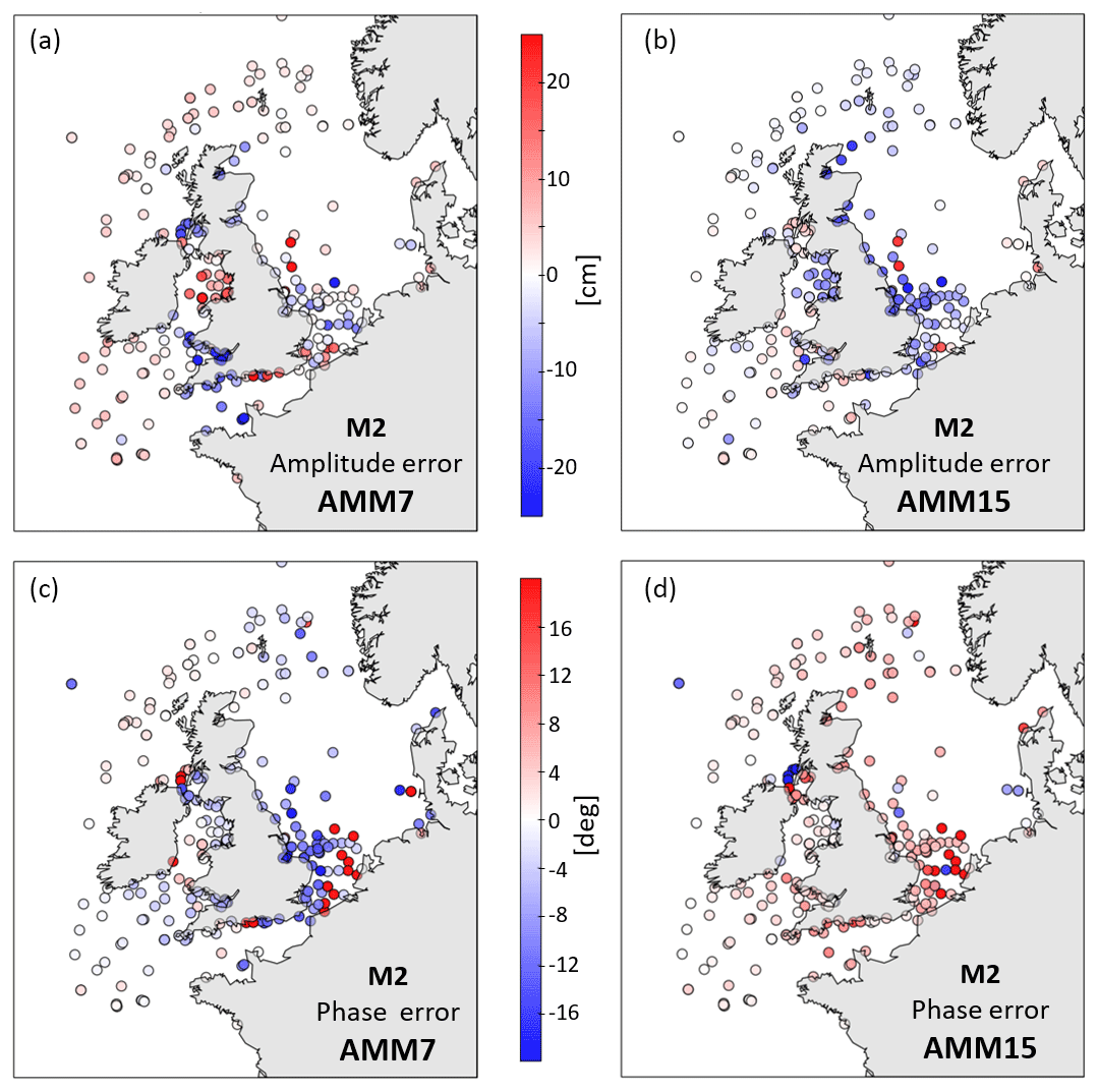
Figure 6M2 amplitude (a, b) and phase (c, d) error relative to observations (observation–model) for AMM7 (a, c) and AMM15 (b, d).
4.1.1 Tidal harmonics
A harmonic analysis of the dominant tidal constituents was compared against tide gauge observations from BODC (British Oceanographic Data Centre; https://www.bodc.ac.uk/data/hosted_data_systems/sea_level/, last access: 15 August 2019) and NOOS (North West Shelf Operational Oceanographic Service; http://noos.eurogoos.eu/, last access: 15 August 2019). The number of tide gauges taken into consideration for AMM15 and AMM7 is the same; therefore, the coastal data, not resolved by the AMM7 coastline, are not taken into consideration. AMM15 has a high horizontal resolution, but since the model applies a minimum depth of 10 m (same as AMM7), the inaccuracy in depth can still affect its ability to properly estimate the tidal speed very close to the coast (Graham et al., 2018a). The statistics for the seven dominant tidal constituents are detailed in Table 8. The differences in amplitude between AMM7 and AMM15 are small. AMM15 has consistently lower RMSD for the phase of the tide, although the phase bias is similar or higher in AMM15.
Table 8RMSD and bias of the tidal amplitude and phase of the prevalent tidal constituents. The values are means over 292 tide gauges for both AMM7 and AMM15. The values in bold indicate an improvement.
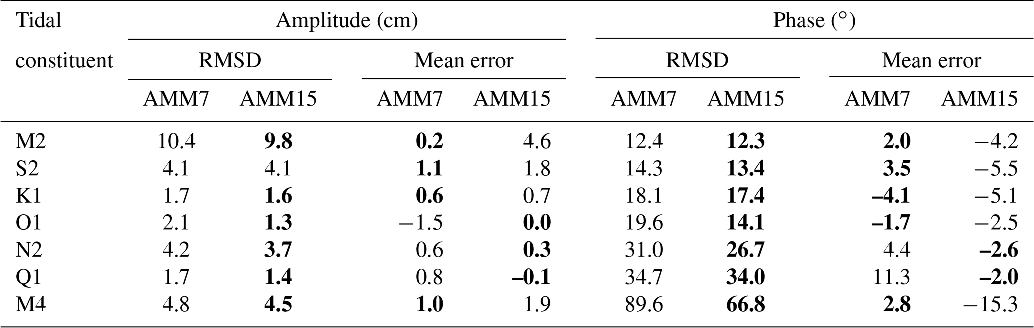
While the performance of AMM7 and AMM15 is similar (Table 7) for basin means, anomalies vary across the domain, showing regional improvements (Graham et al., 2018a). Figure 6 shows the spatial distribution of the M2 tidal errors in the two models. The values of rms and mean error (observation–model) for amplitude and phase are very similar.
The M2 amplitude tends to be somewhat underestimated in the south-west part of the North Sea and along the east coast of the UK. Phase errors, in both models, are largest in the southern North Sea and off the north-eastern coast of Northern Ireland. The AMM15 M2 amplitude is more accurate in the western part of the basin, in particular around the Kintyre Peninsula, as already described in Graham et al. (2018a), and in the Bristol Channel area. The AMM15 phase error is smaller than AMM7 in the German Bight (south-east North Sea) but not in amplitude.
There are no significant differences in the co-tidal chart (not shown) between AMM7 and AMM15; both are very similar to the charts shown in Graham et al. (2018a).
4.1.2 Tidal flow
A month, March 2017, of HF radar surface current velocity data was used to compare AMM7 and AMM15 in the German Bight where the bathymetry is shallow (Fig. 1) and AMM15 is expected to perform better. The total surface velocity data from the COSYNA observing network (Gurgel et al., 2011), available through the EMODnet physics data portal, are computed from radials of three HF radars installed on the islands of Sylt and Wangerooge, and in Büsum (as shown in Fig. 5). Data are averaged every 20 min on a grid of resolution of ∼3 km. At the operating frequencies used, the total surface velocities represent an integrated velocity over a depth between 1 and 2 m. Relative error provided with the data set was used to keep only data with error smaller than 15 %. Model output was interpolated at the time and locations when and where observations were available, to avoid applying gap-filling technics. Temporal coverage over the domain is larger than 75 % everywhere except along the baseline between Büsum and Wangerooge, where the temporal coverage is ∼29 %.
Because the high-frequency variability of the flow in the German bight is dominated by tidal flow, a low-pass filter was applied to the data with gaps, to separate the tidal and the residual component of the velocity. The tidal flow assessment presented here uses the high-pass-filtered data (Fig. 7); the residual currents that come from the low-pass-filtered data are discussed next in Sect. 4.2. Vector correlation (or complex correlation of u+iv, where u and v are the zonal and meridional velocity, respectively, and i is the square root of −1) was estimated and is displayed as correlation amplitude, and phase, or veering. The phase represents the rotation between the two vectors that gives the highest correlation.
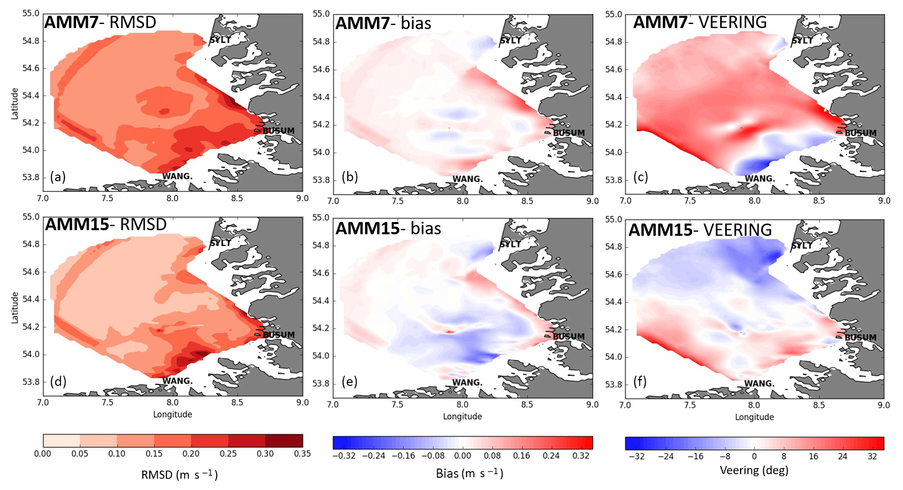
Figure 7Plots of statistics between HF radar surface current observations and AMM7 (a–c) and AMM15 (d–f) for the high-pass-filtered data (tidal signal). Bias (observation–model) and RMSD (in m s−1) are estimated on the velocity vector magnitudes. (c, f) Phase or veering. Positive (negative) veering represents a clockwise (anti-clockwise) angle of AMM7 (a–c) or AMM15 (d–f) vectors with respect to the HF radar vectors. SYLT, WANG, and BUSUM show the locations of the three HF radars on the islands of Sylt and Wangerooge, and in Büsum, respectively.
The various metrics show that AMM15 resolved the tidal current in the south German Bight better than AMM7, as shown in Fig. 7. Although AMM15 bias is slightly higher than that of AMM7 in some areas, RMSD of AMM15 is smaller than the RMSD of AMM7 everywhere in the HF radar domain.
Both models show high correlation with the observations (not shown) and AMM15 has a lower phase, veering, with the observations. Because tidal velocities are rotating periodic signals, the spatial angular veering estimated using the complex correlation can also be interpreted as a temporal phase of the tidal signal. A positive veering angle means that the model tidal velocities lead the HF radar tidal velocities. Figure 7 shows that the tidal phase is improved in AMM15 compared to AMM7 in most of the domain, consistent with the results of the comparison with the tide gauges (Sect. 4.1.1).
4.2 Surface currents in the German Bight
A good forecast of the intensity and direction of the currents is needed for operations at sea, but the validation of this variable is particularly difficult due to the scarcity of observations. There are very few measurements of velocity in the model domain. Among the few data available, we have decided to use the surface currents measured by the HF radar.
The HF radar data used here are 1 month of total surface velocity currents estimated from three HF radar installed in the German Bight, described in the section above (Sect. 4.1.2).
Because the high-frequency variability of the flow in the German Bight is tidally dominated, a low-pass filter was used to separate the tidal and the residual component of the velocity. Statistics were computed on the high-pass- and low-pass-filtered velocity components to assess the tidal and residual flow, respectively. The assessment of the tidal flow is described in Sect. 4.1.2, while this section focuses on the subtidal circulation.
The strong tidal signal in the shallow German Bight results in Kelvin waves propagating eastward on the southern boundary along Germany and northward at the eastern boundary along Denmark. However, this cyclonic circulation may not dominate, as other processes are also influencing the circulation, such as topographic effects from the shallow basin, wind, and stratification resulting from freshwater input mostly from the Elbe and Weser river discharge. Wind tends to also produce a residual cyclonic circulation (Schrum, 1997; Dick et al., 2001; Port et al., 2011). During the month of March 2017, a weak cyclonic circulation was observed in the mean HF radar surface currents along the German and Danish coasts. It is also observed in the AMM15 simulations and as a weaker flow in AMM7. The strong flow out of the Elbe estuary is evident in AMM15 current pattern, even if shifted to the west. AMM7 shows an intensification of its currents in this area but with a speed much smaller than the observations and AMM15 (Fig. 8). Generally, the spatial variability observed in HF radar is better captured by AMM15 than by AMM7. Similar statistics to those estimated for the tidal flow (Fig. 7) also show improvement in both amplitude and direction of the residual flow (not shown).
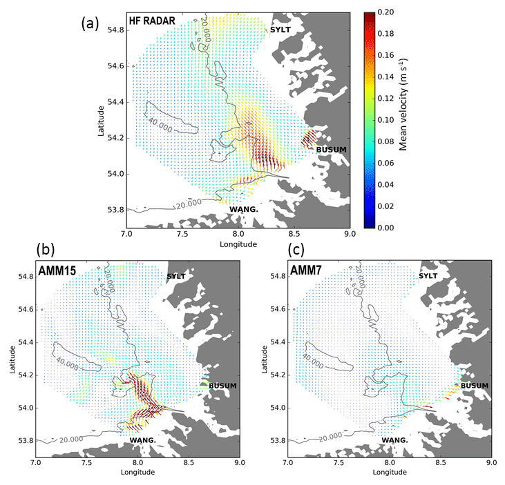
Figure 8March 2017 average surface flow for HF radar (a), AMM7 (b), and AMM15 (c). Model data are regridded on the HF radar grid using cubic interpolation. The hourly model output is linearly interpolated every minute to match the HF radar observations. Model output is only plotted where HF radar data are available. Grey lines represent the 20 and 40 m isobaths. SYLT, WANG, and BUSUM show the locations of the three HF radars on the islands of Sylt and Wangerooge, and in Büsum, respectively.
4.3 Sea surface height
AMM15 and AMM7 SSH is assessed against the satellite SLA data used for the data assimilation both on and off the shelf (Table 7), matching the model to the observation before the SSH data assimilation. The matchups are created by interpolating the model field to the observation location at the model time step nearest to the time of the observations. It is worth noting that the assimilation of SLA is done only where the bathymetry is deeper than 700 m; therefore, no observations are assimilated on-shelf and in a large part of the off-shelf region. The differences between AMM15 and AMM7 are negligible both on the continental shelf and off-shelf. As expected in a tidally dominated area, on the continental shelf the RMSD is slightly higher than off-shelf: 0.13 m on-shelf and 0.09 off-shelf. Both models are overestimating SSH on the shelf, but AMM15 has a smaller bias (−0.02 m for AMM15 and −0.06 m for AMM7). Instead, off-shelf AMM15 and AMM7 have the same absolute value of bias (0.01 m) but opposite sign: positive for AMM15 and negative for AMM7.
4.4 Sea surface temperature
Sea surface temperature is one of the key parameters of heat exchange at the air–sea boundary. Thanks to satellite and in situ observations, SST is the variable with the best measurement coverage in our model domain. SST data are assimilated in the AMM15 and AMM7 models (Fig. 4) during the incremental analysis update (IAU) step of each model run. As a result, an assessment of the model skill at predicting SST compared to observations would be expected to produce a positive result. We have compared the model against all the assimilated observations, the OSTIA products, and a number of time series at selected moorings. It is worth noticing that while the comparison with the assimilated observations is done using the model output at the nearest time step, the comparison against OSTIA is done using the daily means. The hourly instantaneous fields are used instead for the comparison at the mooring locations. This validation allows us to have a general overview of the model SST performance with a detailed analysis of the high-resolution model in few selected locations.
4.4.1 Comparison with in situ and satellite
Model SST has been assessed here against in situ SST measurements matching the model to the observation before the data assimilation, at the model time step closer to the observation time. The in situ measurements are from different instruments, as detailed in Table 3. The number of the in situ SST observations is pretty good during the 2 years: ∼1000 observations per day on the full model domain of which ∼500 are on-shelf. The differences between the two systems, in the full model domain, are very small (Table 7). The RMSD is ∼0.5 ∘C for both AMM7 and AMM15. Both models have a small warm bias, −0.0 ∘C, over the full period. The warm bias is mainly due to the winter months when the model is slightly warmer than the observations. The same statistics on-shelf show very similar results.
In addition to the in situ observation assessment, the model hourly SSTs have been compared to the Met Office's OSTIA system (Donlon et al., 2012). OSTIA provides analyses of the foundation SST (i.e. the SST free of diurnal variability) and assimilates in situ and satellite observations. The OSTIA data, available through the CMEMS catalogue, are produced on a 1∕20∘ grid (∼6 km resolution); however, this is not the feature resolution of the product, which depends on other aspects of the system such as the correlation length scales used in producing the analysis. OSTIA has a maximum feature resolution of ∼20–30 km and so both AMM7 and AMM15 are expected to represent smaller features than OSTIA. The important point to consider in this assessment is that OSTIA foundation SST is being compared to the model surface box daily mean SST that should be biased warm compared to the foundation.
The reference grid used for the intercomparison of these three data sets is AMM7; therefore, OSTIA and AMM15 have been interpolated at 7 km.
The bias is defined as observation–model. Both models are biased warm compared to OSTIA (Fig. 9), in agreement with the in situ–model matchup statistics. AMM15 has a slightly higher bias than AMM7 but the same RMSD. The high variability of the signal in AMM15 could be penalized by the interpolation onto a grid at lower resolution. Overall, we see little difference in performance between the two systems. The mean RMSD for the period 2016–2017 is for both systems of 0.3 ∘C, smaller than the RMSD computed by the in situ–model matchup statistics (0.5 ∘C). The comparison between OSTIA–model and in situ–model differs also because OSTIA comparison uses a full field to calculate the statistics rather than the single-point observation used in the in situ–model matchups.

Figure 9OSTIA minus model SST RMSD and bias daily comparison for AMM7 (blue) and AMM15 (red) for the whole domain (negative mean error indicates a warm model bias).
4.4.2 Variability in SST
A small number of buoys have been used to investigate the SST variability in the models (Fig. 5). Three sites were investigated in this study: E1 (50.026∘ N, 4.225∘ W) in the English Channel and the FINO sites in the German Bight (FINO 1 at 54∘00.89′ N, 6∘35.26′ E, and FINO 3 at 55∘11.7′ N, 7∘9.5′ E), buoys marked as 1 and 2 in Fig. 5. In the future, it would be helpful to get a broader range of sites included. A Butterworth filter (Butterworth, 1930) has been applied to the hourly model and observed SST data, using a cut-off for the filter at 5 d which removes the large-scale synoptic and seasonal signals, leaving the internal dynamics and the wind-driven signals, as well as the tidal frequencies. The observation data were interpolated hourly to be equivalent to the model data, and the precision of the model data was reduced to the same precision as the observations, to allow direct comparison and to prevent any aliasing. The time series were divided into seasons, both due to the high seasonal variability of SST and to avoid observation data gaps that would skew the analysis. We defined the four seasons as December–January–February (DJF), March–April–May (MAM), June–July–August (JJA), and September–October–November (SON). The data used for this study cover the period of December 2016–November 2017.
The model data were taken from the analysis day. It would be interesting to also assess the forecast; this will be the subject of future studies. Figure 10 shows the SST and filtered SST time series at the FINO 3 mooring for two different seasons, winter (DJF) and summer (JJA). The filtered SST signal has a higher variability in summer when the diurnal warming is stronger, and therefore the SST gradients are bigger. AMM7 and AMM15 have very similar values of SST, probably due to the data assimilation of SST that brings both models close to the observations.
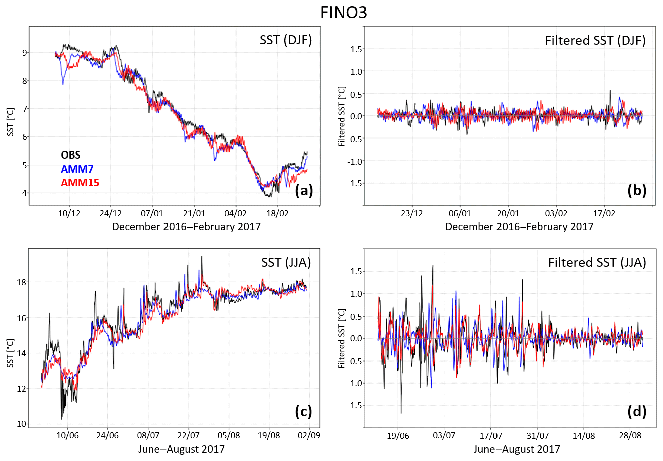
Figure 10Time series of sea surface temperature (a, c) and filtered SST (b, d) for the FINO 3 buoy for December 2016–February 2017 (a, b) and June–August 2017 (c, d). Observations are shown in black, AMM7 in blue, and AMM15 in red.
Spectral powers were estimated and smoothed using a Loess filter to remove noise in the spectra. Figure 11 shows the power spectra for each season at the FINO 3 buoy; the non-filtered spectra are also plotted as faint lines. The power spectra of SST at the other mooring locations, E1 and FINO 1, are not shown but are similar to FINO 3. Although this is not exclusively true, the general trend is for the models to drop off in power more quickly with frequencies, and have a steeper spectral slope, than the observations. AMM15 SST is more variable at frequency higher than daily, although at periods of 4 h and lower the models tend to behave quite similarly. This is consistent with what one would expect from the mesoscale resolving skills of AMM15. This high-frequency increase of variability in AMM15 compared to AMM7 can also be seen by quantitative inspection of the model fields (Fig. 10), with small length scale features being more prevalent in AMM15. At higher frequencies (shorter periods), SST spectra for both models collapse to the same power spectrum value with generally less variability than the observations at high frequencies.
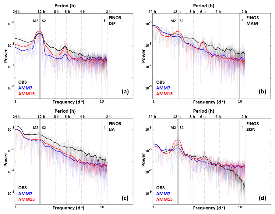
Figure 11Power spectrum of SST for the FINO 3 buoy (black line) compared with the AMM7 (blue) and AMM15 (red) simulations for December 2016 to February 2017 (a), March to May 2017 (b), June to August 2017 (c), and September to November 2017 (d).
This suggests that on average some of the very high-frequency/small-scale features are still not being represented in the models, although it should be noted that the model represents a mean over a grid which will by definition introduce some smoothing, whereas the observations are (at least to a greater extent) sampling at a point. This analysis demonstrates quantitatively that the AMM15 better represents the high-frequency/small-scale features, which can visually be observed from model fields' time series but are poorly assessed through global statistics, as shown in Table 7. This result is likely to be even more pronounced in forecast fields, although that is not demonstrated here.
4.5 Water column
4.5.1 Temperature and salinity profiles
AMM15 shows improved vertical structure of the water column, with a lower bias and RMSD compared to AMM7 in salinity and temperature. Figure 12 shows the mean error (observation–model) and the RMSD averaged over the whole domain, with observation–model differences calculated before the assimilation of the vertical profiles. The temperature bias of both models is very small at the surface but increases below 100 m. Between 500 and 1000 m, AMM15 has a mean error close to zero, while AMM7 has a cold bias. AMM15 also has a lower RMSD than AMM7 at all depths below the surface. The distribution of the subsurface observations, shown in Fig. 4, is uneven, with very few observations on-shelf; therefore, it is not possible to distinguish between the water column improvements off-shelf and on-shelf using this technique, and these improvements are demonstrated predominantly for the off-shelf region. This is a very good result considering that the skills in modelling salinity and temperature depth structure have recently been significantly improved in AMM7 with the improvements in data assimilation, with the addition to SST of SLA and subsurface profiles (King et al., 2018). This means that, in less than 2 years, the NWS system has consistently improved its skill in resolving the vertical profiles of temperature and salinity and therefore the density of the water column.
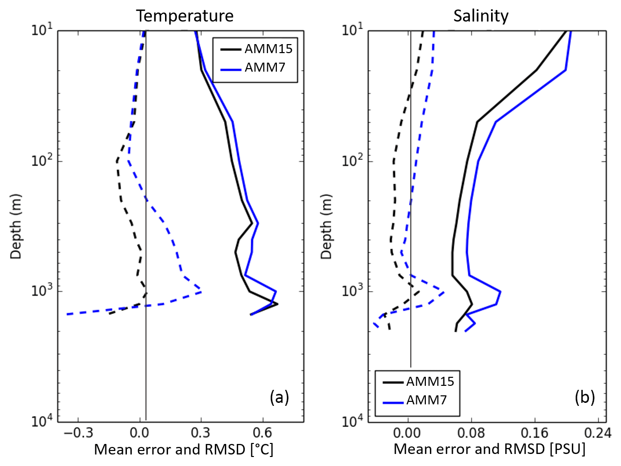
Figure 12Observation minus model temperature (a) and salinity (b) profile assessment for AMM15 (black) and AMM7 (blue) for the whole domain. The RMSD is shown by the solid lines and mean error (observation–model) is shown by the dashed lines.
4.5.2 Moorings in the German Bight
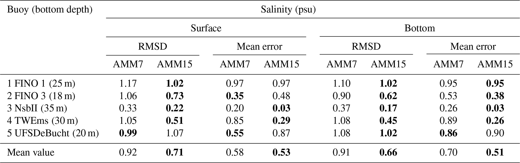
Tables 9 and 10 show the temperature and salinity statistics for the model and observations comparison during the year 2017 at the five moorings in the German Bight (Fig. 5). Observations for both temperature and salinity are available at surface (5 m) and bottom. The models assimilate only SST observations, not salinity, and no bottom observations. The hourly instantaneous model data are compared to the buoy observations with a few discontinuities due to missing measurements during a short period of the year. AMM15 has a better RMSD and a lower error mean at all buoy locations. The high-frequency variability is better reproduced by AMM15 than AMM7, as shown in Fig. 13 for the surface salinity field in the NsbII (mooring no. 3 in the map in Fig. 5).
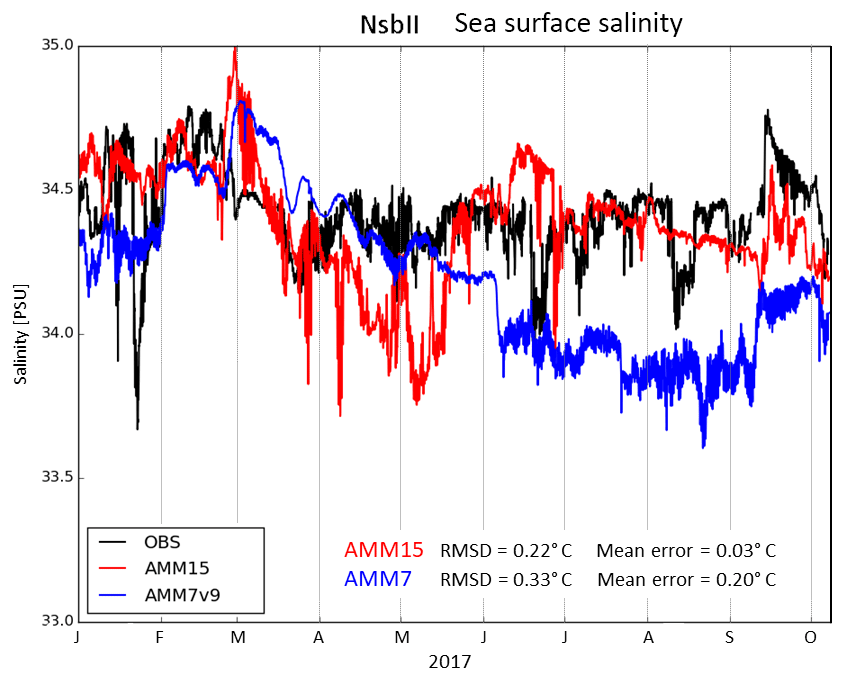
Figure 13Sea surface salinity at the NsbII mooring for January–September 2017. The black line represents the observations; the red and the blue lines represent AMM15 and AMM7, respectively. Observations are missing for the period of October–December.
Table 9Yearly mean (2017) RMSD and bias statistics at the five moorings in the German Bight (observation–model). Surface and bottom temperature are for AMM7 and AMM15. The values in bold indicate an improvement.
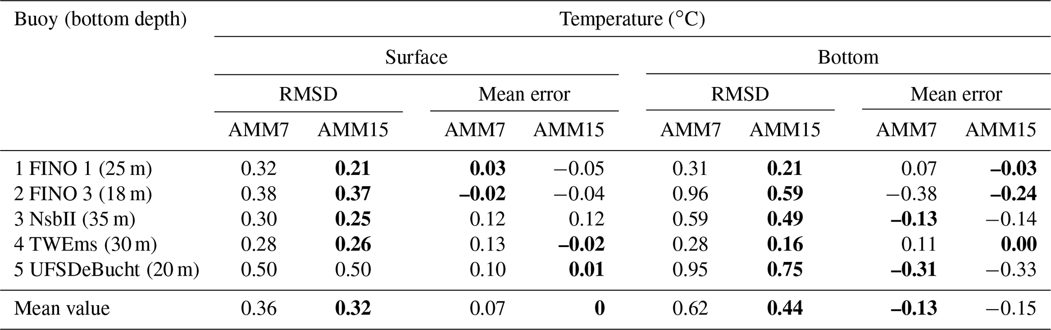
Table 10Yearly mean (2017) RMSD and bias statistics at the five moorings in the German Bight (observation–model). Surface and bottom salinity are for AMM7 and AMM15. The values in bold indicate an improvement.
Temperature RMSD and bias are very small at surface due to the strong constraint of the data assimilation of SST (as described in Sect. 4.3), while at the bottom AMM15 is more accurate in prescribing the temperature at all mooring locations (Table 9).
AMM7 and AMM15 both have high salinity errors in the German Bight, as highlighted by the comparison with the buoys that are located closer to the coast (FINO 1, FINO 3, and UFSDeBucht). This is most probably due to representation of river discharge. AMM15 performs better than AMM7, probably because it is less diffusive within river plumes and has a lower lateral diffusion. Improved bathymetry and coastal resolution are also likely to play a role in coastal areas with depth less than 20 m. AMM15 has halved the salinity error compared to AMM7 when compared with the outer buoys (NsbII and TWEms). It is encouraging to see that AMM15 is better than AMM7 at the bottom at all mooring locations. The decision to use the climatological river discharge data set instead of E-Hype for AMM7, and subsequently AMM15, has improved salinity remarkably in the German Bight, reducing the model fresh bias. This modification was implemented in April 2017, meaning that we have significantly improved the salinity in the last two major updates of the NWS forecasting system. Nevertheless, using a climatological river runoff data set is a limitation for a high-resolution forecasting system, affecting variability in coastal water properties. Finding a suitable alternative will be a priority for future releases of this system.
Temperature RMSD and bias are very small at the surface due to the strong constraints of the data assimilation of SST (as described in Sect. 4.3), while at the bottom AMM15 is more accurate in prescribing the temperature at all mooring locations (Table 9).
4.5.3 Glider transects
AMM15 and AMM7 vertical structure and high-frequency variability is assessed against the glider profiles from MASSMO (Marine Autonomous Systems in Support of Marine Observations), Mission4 (Figs. 5 and 14). MASSMO is a pioneering multi-partner series of trials and demonstrator missions that aims to explore the UK seas using a fleet of innovative marine robots. With newly developed unmanned surface vehicles (USVs) and submarine gliders, the multi-phase project has successfully completed the largest single deployment of marine autonomous systems ever seen in the UK. In the summer of 2017, a fleet of 11 autonomous marine robots was deployed to explore the seas north-west of the Orkney Islands in search of marine mammals and sources of man-made noise pollution. The mission was part of an annual series of marine robot trials coordinated by the National Oceanography Centre in partnership with 16 organizations representing UK government, research, and industry (http://projects.noc.ac.uk/massmo, last access: 15 August 2019). The fleet comprised eight submarine gliders and three unmanned surface vehicles, travelling up to 200 km offshore to the Faroe–Shetland Channel where water depths exceeded 1000 m. The MASSMO4 campaign covered the period 22 May to 6 June 2017 with three gliders deployed north of Scotland, close to the coast, and then travelled across the shelf break.

Figure 14Glider 553 trajectory. The glider started the measurements close to the Scotland coast and then moved towards the shelf break. The black line is the glider trajectory. The grey line represents the 200 m isobath. The red dot is the glider position on 23 May 2017. The field in the background is the AMM15 salinity on 23 May at 30 m.
The MASSMO4 data set is therefore a very high-resolution source of information in a key area of the model domain. We have compared the models and observations along the glider track, using the model high-frequency data (hourly instantaneous fields). Figure 14 shows the trajectory of one of these gliders (553), which was measuring temperature and salinity from surface to bottom. The background field in this figure shows surface salinity from AMM15 at 12:00 UTC on 23 May, when the glider was in the position marked by the red dot.
AMM15 is in very good agreement with the observations and shows improvement, compared to AMM7 (Figs. 15 and 16), particularly for salinity along the glider trajectories. The only exception being the low-salinity pattern in the whole water column measured by the glider around 23 March, when AMM15 is too salty and AMM7 too fresh. It could be due to a misplacement of a front, as suggested by the AMM15 salinity map (Fig. 14). The AMM7 salinity field (not shown) has lower variability and this could justify the smaller misfit compare to the glider in that precise location.
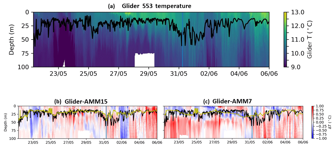
Figure 15Top 100 m of temperature profile along glider 553-100 trajectory. (a) Temperature measured by the glider. (b) Difference between the glider and AMM15. (c) Difference between the glider and AMM7. The vertical blue line represents time when the glider goes over the shelf break, crossing the 200 m isobath. Before that time, the glider is on the shelf. The black line is the MLD computed from the glider measurements; the yellow line is the model MLD.
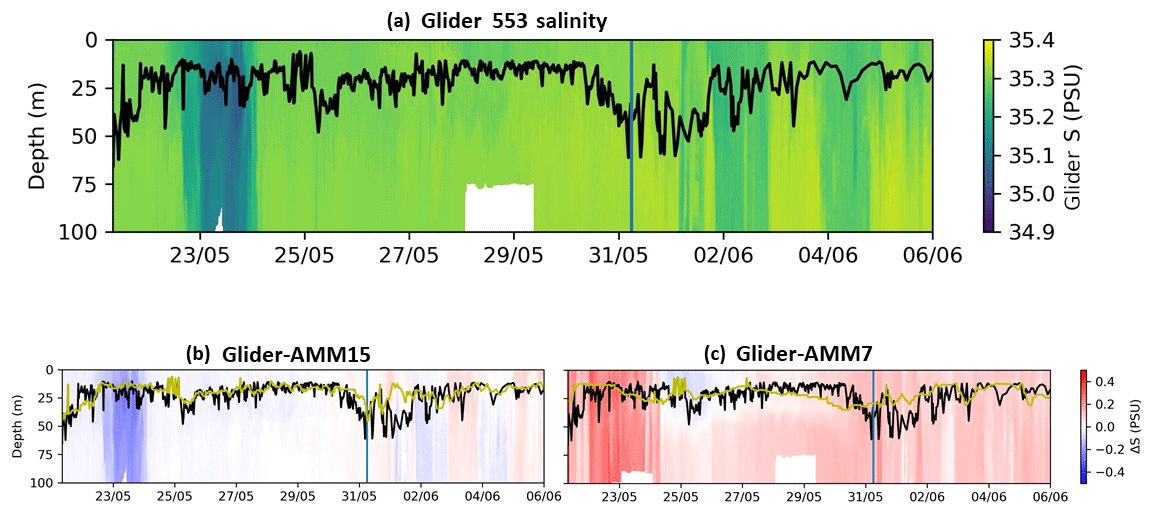
Figure 16Top 100 m of salinity profile along glider 553-100 trajectory. (a) Salinity measured by the glider. (b) Difference between the glider and AMM15. (c) Difference between the glider and AMM7. The vertical blue line represents time when the glider goes over the shelf break, crossing the 200 m isobath. Before that time, the glider is on the shelf. The black line is the MLD computed from the glider measurements; the yellow line is the model MLD.
The salinity field in AMM15 has finer-scale structures and usually the low salinity is better constrained along the coast. The density of the water column during the period of the glider campaign is therefore much more accurate in AMM15 (Fig. 17). While these results may not be representative of the whole model domain or of the seasonal variability in stratification of the water column, they are very encouraging.
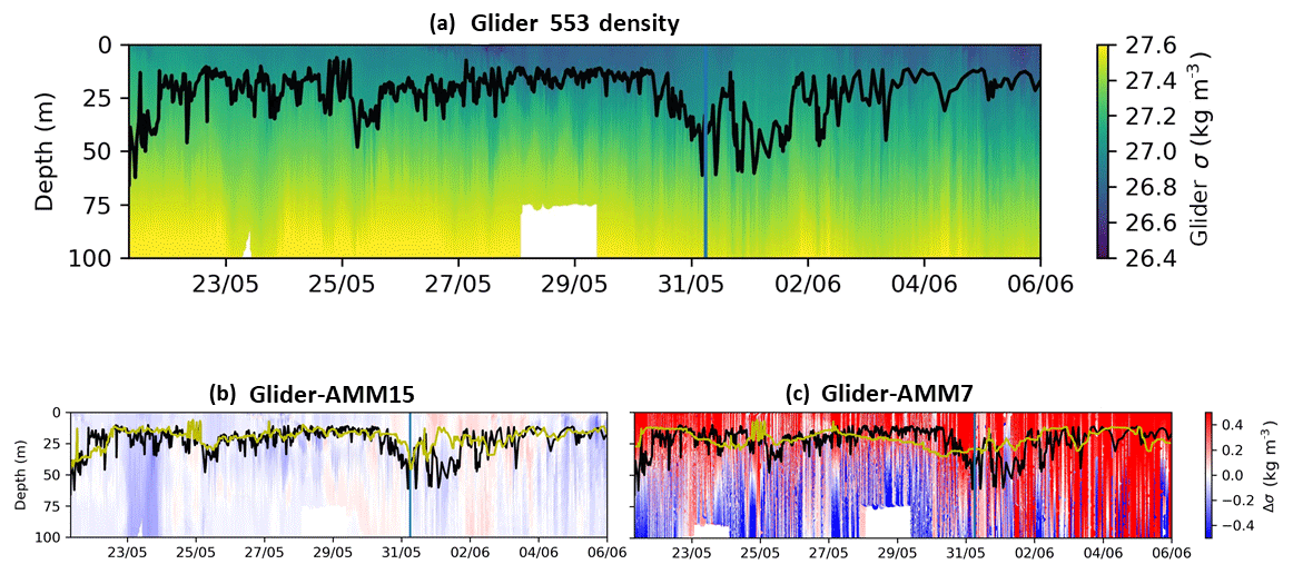
Figure 17Top 100 m density profile along glider 553-100 trajectory. (a) Salinity measured by the glider. (b) Difference between the glider and AMM15. (c) Difference between the glider and AMM7. The vertical blue line represents time when the glider goes over the shelf break, crossing the 200 m isobath. Before that time, the glider is on the shelf. The black line is the MLD computed from the glider measurements; the yellow line is the model MLD.
In all depth profiles for AMM7, there is a white patch close to the bottom on 23 May. This is due to the model bathymetry being shallower than the reality in that specific location. This is a confirmation than AMM15 has a more realistic representation of the bottom topography, as described in Sect. 2.1.
The increased resolution of fine-scale structures in AMM15 results in increased transport across the shelf break, particularly in the region observed here (Graham et al., 2018b). These results, showing AMM15 has improved vertical structure and variability of the water column, support the conclusions of Graham et al. (2018b). Shelf-break processes transporting water masses between the deep ocean and across the shelf will have a strong impact on conditions observed in this region.
4.5.4 Mixed layer depth
The MLD has been calculated within the model using a density criterion, following the definition of Kara et al. (2000), except the reference depth of 10 m is changed to 3 m due to the shallower regions of the continental shelf. The MLD is defined as the depth where the density increases, compared to density at 3 m depth, corresponding to a temperature decrease of 0.2 ∘C in local surface conditions. The EN4 (Good et al., 2013) profile data set of temperature and salinity was used to calculate an “observed” Kara mixed layer depth following the same procedure used within the model.
An important point to note here is that on daily/monthly timescales the EN4 data set is still relatively sparse in the region of interest and often clustered in particular locations. This is particularly true on the continental shelf. Assessing the model as a whole, we see a seasonal cycle of errors with small errors in summer/autumn (bias ∼ 10 m and RMSD < 25 m) and larger errors in winter/spring.
We have therefore also computed the mixed layer depth from the MASSMO4 observations, comparing the mixed layer depth from the gliders (black line in Fig. 17) with AMM15 and AMM7 in the corresponding locations (yellow line in Fig. 17). AMM15 reproduces the mixed layer depth better than AMM7 and represents the variability of the signal very well. This positive result was also true along the other glider trajectories in this region. AMM15, but not AMM7, also reproduces a deepening in the MLD at the shelf break. While this could be just a temporary feature, it could also be explained by increased mixing due to internal waves, which begin to be resolved in AMM15 but not in AMM7 (Guihou et al., 2017). Graham et al. (2018b) also show that the slope current differs between AMM15 and AMM7 in this region, which is likely to affect the water column structure and variability around the shelf break. Differences in currents are also discussed further in the following section.
The validation of pre-operational trial experiments for a new 1.5 km resolution model of the North-West European Shelf, against observations and the predecessor 7 km system, shows positive results.
AMM15 has improved skill compared to AMM7 and has proven to be an improvement especially when compared to high spatial–temporal resolution observations. The pattern and variability of surface currents are better reproduced by the new system, with improved temperature and salinity throughout the whole water column. The most outstanding improvement seems to be in the salinity which is closer to observations at basin scale and locally. Probably there are different factors which contribute to this improvement. Firstly, salinity will be impacted by river runoff. While the two models have a similar daily climatological river runoff data set, it could differ locally. Despite similar runoff, the path of the river plume may also differ in the two models, so it may lead to local changes in salinity, for example, in the German Bight, where the plume stays close to the coast rather than diffusing offshore. Secondly, the Atlantic and Baltic boundaries are in a different geographical location and this could imply differences in the fluxes at the boundary. There is a strong salinity variability at the Baltic boundary and this can strongly influence the salinity field and variability in the North Sea. There are ongoing developments to improve the Baltic boundary implementation in AMM15 that will help to further understand the impact of this boundary on the NWS. The Atlantic boundaries influence the exchange across the shelf and they could be partly responsible for improvements like those shown in the north of Scotland where the model has been compared with glider data and the AMM15 salinity field is much more realistic than AMM7. The significant improvement in this area could also be due to AMM15 better resolving the flow through the Faroe–Shetland Channel and shelf-break exchange. The work from Graham et al. (2018b) shows that there is an increased flux across the shelf break in AMM15 compared to AMM7. This could affect the exchange of water masses around the shelf break and therefore influence salinity on the shelf. Another reason could be the differences in the atmospheric forcing with the two models forced by a different evaporation–precipitation rate. As stated earlier, further studies will be carried out to properly assess the impact of the ECMWF forcing compared to the Met Office forcing.
The assimilation scheme used in AMM15 is broadly unchanged from that used in AMM7. While the short correlation length scale is now ∼5 km (compared to ∼20 km), the observation and background error covariances, and the observation types assimilated, remain unchanged. In this initial implementation of AMM15, we have not attempted to improve the use of observations in the assimilation scheme. We are currently investigating how to adapt our assimilation scheme to assimilate SLA observations in stratified water and will be re-estimating the observation and background error covariances for this new higher-resolution system.
The 1.5 km resolution model provides a better representation of dynamical features such as coastal currents, fronts, and mesoscale eddies that can vary in size from only a few kilometres in shelf seas to tens of kilometres, but a proper assessment is very difficult due to the high variability of these patterns and the very limited number of available observations.
The users' benefit, using the newly improved European shelf product (AMM15), will vary depending on their applications. A positive impact on the users and their application is expected from AMM15 products. Higher-resolution current fields with an improved representation of the coastal areas should improve the results of applications like drifting models simulating pollutant or oil spill dispersion and all the applications that need a high-resolution current field. All the acoustic applications, strongly depending on the density stratification and its variability, will benefit from these new products since they have a better representation of the water masses. A general positive impact is expected for most of the users like public bodies responsible for marine environmental regulation, aquaculture industries, marine renewable oil, and gas industries.
There are some improvements in the tidal signal in AMM15, even if they are not as remarkable as those with the salinity. One limitation is the minimum depth set to 10 m that prevents the model from properly taking into account the shallow bathymetry in the coastal areas. A wetting and drying implementation is under development and could help to have a more realistic bathymetry, with improved tidal signal in very shallow waters, in a future version of AMM15.
AMM15 has been developed with coupled prediction in mind, the domain matching that of the Met Office atmospheric UKV model. Regional coupled model developments have been done and coupled ocean forecasting systems are already planned.
The AMM15 system described in this paper has been already tested in an ocean–wave coupled configuration (Lewis et al., 2019a) which is planned to become operational in 2020. We hope to add the biogeochemical components in a few years, but a precise plan is not yet available. Indeed, a preliminary version of AMM15 with coupled ocean–biogeochemistry is under development with encouraging initial results but is still far from meeting operational requirements. A coupled ocean–atmosphere version of this model has already been developed for research (Lewis et al., 2019b) and studies will continue toward a fully coupled prediction system with an ocean, atmosphere, land, and wave model.
The nature of the 4-D data generated in running the model experiments requires a large tape storage facility. These data are of the order of 2 TB (terabytes). The high-resolution model data, from January 2017 to the present, are available on the CMEMS web portal (http://marine.copernicus.eu, NORTHWESTSHELF_ANALYSIS_FORECAST_PHY_004_013, last access: 16 August 2019). Year 2016 and the low-resolution data for years 2016–2017 can be made available upon request from the authors.
All authors contributed to the scientific evaluation and analysis of the results. In addition, MT designed the experiments and their validation strategy. PS developed the technical configurations used and supported running the simulations. RK developed the NEMO regional ocean assimilation system and supported running the simulations. NM supported running the simulations and undertook the validation of the tidal harmonics. ACP undertook the evaluation against glider and HF radar observations. JS undertook the SST variability assessment. EO and JG provided detailed information on the NEMO configuration used in these experiments.
The authors declare that they have no conflict of interest.
This article is part of the special issue “The Copernicus Marine Environment Monitoring Service (CMEMS): scientific advances”. It is not associated with a conference.
Funding support from the Copernicus Marine Environment Monitoring Service and the UK Ministry of Defence is gratefully acknowledged.
This paper was edited by Markus Meier and reviewed by one anonymous referee.
Berg, P. and Weismann Poulsen, J.: Implementation details for HBM, DMI Technical Report No. 12-11, available at: https://www.dmi.dk/fileadmin/Rapporter/TR/tr12-11.pdf (last access: 15 August 2019), 2012.
Bloom, S. C., Takacs, L. L., da Silva, A. M., and Ledvina, D.: Data Assimilation Using Incremental Analysis Updates, Mon. Weather Rev., 124, 1256–1271, https://doi.org/10.1175/1520-0493(1996)124<1256:DAUIAU>2.0.CO;2, 1996.
Brassington, G.: Forecast Errors, Goodness, and Verification in Ocean Forecasting, J. Mar. Res., 75, 403–433, https://doi.org/10.1357/002224017821836851, 2017.
Burchard, H. and Bolding, K.: GETM, A General Estuarine Transport Model: Scientific Documentation, Tech. Rep. EUR 20253 EN, Eur. Comm., Ispra (VA), Italy, available at: https://publications.europa.eu/en/publication-detail/-/publication/5506bf19-e076-4d4b-8648-dedd06efbb38 (last access: 15 August 2019), 2002.
Burrows, M. and Thorpe, S. A.: Drifter observations of the Hebrides slope current and nearby circulation patterns, Ann. Geophys., 17, 280–302, 1999.
Butterworth, S.: On the theory of Filter Amplifiers, in: Experimental Wireless and the Wireless Engineer, Vol. 7, Ilife & Sons Limited, London, 536–541, September 1930.
Dick, S., Eckard, K., Müller-Navarra, S., Klein, H., and Komo, H.: The operational circulation model of BSH (BSHcmod) – model description and validation, Berichte des Bundesamtes für Seeschifffahrt und Hydrographie (BSH) 29, Bundesamt für Seeschifffahrt und Hydrographie, Hamburg, Rostock, available at: https://www.bsh.de/DE/PUBLIKATIONEN/_Anlagen/Downloads/Meer_und_Umwelt/Berichte-des-BSH/Berichte-des-BSH-56.html;jsessionid=A6966DF5C4E4B4E8DEE7DA32C7930E6A.live11292?nn=1907948 (last access: 15 August 2019), 2001.
Donlon, C. J., Martin, M., Stark, J., Roberts-Jones, J., Fiedler, E., and Wimmer, W.: The Operational Sea Surface Temperature and Sea Ice Analysis (OSTIA) system, Remote Sens. Environ., 116, 140–158, 2012.
Egbert, G. D. and Erofeeva, S. Y.: Efficient Inverse Modeling of Barotropic Ocean Tides. J. Atmos. Ocean. Tech., 19, 183–204, https://doi.org/10.1175/1520-0426(2002)019<0183:EIMOBO>2.0.CO;2, 2002.
Fairall, C. W., Bradley, E. F., Hare, J. E., Grachev, A. A., and Edson, J. B.: Bulk Parameterization of Air–Sea Fluxes: Updates and Verification for the COARE Algorithm, J. Climate, 16, 571–591, https://doi.org/10.1175/1520-0442(2003)016<0571:BPOASF>2.0.CO;2, 2003.
Flather, R. A.: A tidal model of the north west European continental shelf, Memoires de la Société Royale de Sciences de Liege, 6, 141–164, 1976.
Flather, R. A.: Results from a model of the north east Atlantic relating to the Norwegian Coastal Current. The Norwegian Coastal Current (Proceedings from the symposium, Geilo, 9–12 September 1980), Bergen University, Bergen, 2, 427–458, 1981.
Good, S. A., Martin, M. A., and Rayner, N. A.: EN4: quality controlled ocean temperature and salinity profiles and monthly objective analyses with uncertainty estimates, J. Geophys. Res.-Oceans, 118, 6704–7616, 2013.
Graham, J. A., O'Dea, E., Holt, J., Polton, J., Hewitt, H. T., Furner, R., Guihou, K., Brereton, A., Arnold, A., Wakelin, S., Castillo Sanchez, J. M., and Mayorga Adame, C. G.: AMM15: a new high-resolution NEMO configuration for operational simulation of the European north-west shelf, Geosci. Model Dev., 11, 681–696, https://doi.org/10.5194/gmd-11-681-2018, 2018a.
Graham, J., Rosser, J. P., O'dea, E., and Hewitt, H. T.: Resolving the Shelf Break Exchange Around the European Northwest Shelf, Geophys. Res. Lett., 45, https://doi.org/10.1029/2018GL079399, 2018b.
Guihou, K., Polton, J., Wakelin, S., O'Dea, E., and Holt, J.: Kilometric Scale modeling of the North West European Shelf Seas: Exploring the spatial and temporal variability of internal tides, J. Geophys. Res.-Oceans, 123, 688–707, https://doi.org/10.1002/2017JC012960, 2017.
Gurgel, K. W., Schlick, T., Voulgaris, G., Seemann, J., and Ziemer, F.: HF radar observations in the German Bight: Measurements and quality control, in: 2011 IEEE/OES 10th Current, Waves and Turbulence Measurements (CWTM), March 2011, Monterey, California, USA, 51–56, 2011.
Holt, J., Hyder, P., Ashworth, M., Harle, J., Hewitt, H. T., Liu, H., New, A. L., Pickles, S., Porter, A., Popova, E., Allen, J. I., Siddorn, J., and Wood, R.: Prospects for improving the representation of coastal and shelf seas in global ocean models, Geosci. Model Dev., 10, 499–523, https://doi.org/10.5194/gmd-10-499-2017, 2017.
Holt, J. T. and James, I. D.: An s coordinate density evolving model of the northwest European continental shelf: 1. Model description and density structure, J. Geophys. Res.-Oceans, 106, 14015–14034, https://doi.org/10.1029/2000JC000304, 2001.
Holt, J. T. and Umlauf, L.: Modelling the tidal mixing fronts and seasonal stratification of the Northwest European Continental shelf, Cont. Shelf Res., 28, 887–903, https://doi.org/10.1016/j.csr.2008.01.012, 2008.
Ikeda, M., Johannessen, J. A., Lyge, K., and Sandven, S.: A Process Study of Mesoscale Meanders and Eddies in the Norwegian Coastal Current, J. Phys. Oceanogr., 19, 20–35, 1989.
Ingleby, B. and Huddlestone, M.: Quality control of ocean temperature and salinity profiles – Historical and real-time data, J. Mar. Syst., 65, 158–175, https://doi.org/10.1016/j.jmarsys.2005.11.019, 2007.
Kara, A. B., Rochford, P. A., and Hurlburt, H. E.: An optimal definition for ocean mixed layer depth, J. Geophys. Res., 105, 16803–16821, https://doi.org/10.1029/2000JC900072, 2000.
King, R., While, J., Martin, M. J., Lea, D. J., Lemieux-Dudon, B., Waters, J., and O'Dea, E.: Improving the initialisation of the Met Office operational shelf-seas model, Ocean Model., 130, 1–14, 2018.
Large, W. and Yeager, S.: The global climatology of an interannuallly varying air-sea data set, Clim. Dynam., 33, 341–364, 2009.
Lea, D. J., Drecourt, J. P., Haines, K., and Martin, M. J.: Ocean altimeter assimilation with observational- and model-bias correction, Q. J. Roy. Meteorol. Soc., 134, 1761–1774, https://doi.org/10.1002/qj.320.2008, 2008.
Le Traon, P. Y., Ali, A., Alvarez Fanjul, E., Aouf, L., Axell, L., Aznar, R., Ballarotta, M., Behrens, A., Benkiran, M., Bentamy, A., Bertino, L., Bowyer, P., Brando, Breivik, L. A., Buongiorno Nardelli, B., Cailleau, S., Ciliberti, S. A., Clementi, E., Colella, S., Mc Connell, N., Coppini, G., Cossarini, G., Dabrowski, T., de Alfonso Alonso-Muñoyerro, M., O'Dea, E., Desportes, C., Dinessen, F., Drevillon, M., Drillet, Y., Drudi, M., Dussurget, R., Faugère, Y., Forneris, V., Fratianni, C., Le Galloudec, O., García-Hermosa, M. I., García Sotillo, M., Garnesson, P., Garric, G., Golbeck, I., Gourrion, J., Grégoire, M. L., Guinehut, S., Gutknecht, E., Harris, C., Hernandez, F., Huess, V., Johannessen, J. A., Kay, S., Killick, R. King, R., de Kloe, J., Korres, G., Lagemaa, P., Lecci, R., Legeais, J. F., Lellouche, J. M., Levier, B., Lorente, P., Mangin, A., Martin, M., Melet, A., Murawski, J., Özsoy, E., Palazov, A., Pardo, S., Parent, L., Pascual, A., Paul, J., Peneva, E., Perruche, C.,, Peterson, D., Petit de la Villeon, L., Pinardi, N., Pouliquen, S., Pujol, M. I., Rainaud, R., Rampal, P., Reffray, G., Regnier, C., Reppucci, A., Ryan, A., Salon, S., Samuelsen, A., Santoleri, R., Saulter, A., She, J., Solidoro, C., Stanev, E., Staneva, J., Stoffelen, A., Storto, A., Sykes, P., Szekely, T., Taburet, G., Taylor, B., Tintore, J., Toledano, C., Tonani, M., Tuomi, L., Volpe, G., Wedhe, H., Williams, T., Vandendbulcke, L., van Zanten, D., von Schuckmann, K., Xie, J., Zacharioudaki, A., and Zuo, H.: The Copernicus Marine Environmental Monitoring Service: Main Scientific Achievements and Future Prospects, Special Issue Mercator Océan Journal, 56, 46–50, https://doi.org/10.25575/56, 2017.
Lewis, H., Castillo Sanchez, J. M., Siddorn, J., King, R., Tonani, M., Saulter, A., Sykes, P., Péquignet, A.-C., Weedon, G., Palmer, T., Staneva, J., and Bricheno, L.: Can wave coupling improve operational regional ocean forecasts for the North-West European Shelf, Ocean Sci., 15, 669–690, https://doi.org/10.5194/os-15-669-2019, 2019a.
Lewis, H., Siddorn, J., Castillo Sanchez, J. M., Petch, J., Edwards, J., and Smyth, T.: Evaluating the impact of atmospheric forcing resolution and air–sea coupling on near-coastal regional ocean prediction, Ocean Sci., 15, 761–778, https://doi.org/10.5194/os-15-761-2019, 2019b.
MacLachlan, C., Arribas, A., Peterson, K. A., Maidens, A., Fereday, D., Scaife, A. A., Gordon, M., Vellinga, M., Williams, A., Comer, R. E., Camp, J., Xavier, P., and Madec, G.: Global Seasonal forecast system version 5 (GloSea5): a high-resolution seasonal forecast system, Q. J. Roy. Meteorol. Soc., 141, 1072–1084, https://doi.org/10.1002/qj.2396, 2015.
Madec, G. and the NEMO team: NEMO ocean engine, Note du Pôle de modélisation, No. 27, Institut Pierre-Simon Laplace (IPSL), France, ISSN 1288-1619, 2016.
Marsh, R., Haigh, I. D., Cunningham, S. A., Inall, M. E., Porter, M., and Moat, B. I.: Large-scale forcing of the European Slope Current and associated inflows to the North Sea, Ocean Sci., 13, 315–335, https://doi.org/10.5194/os-13-315-2017, 2017.
Mirouze, I., Blockley, E. W., Lea, D. J., Martin, M. J., and Bell, M. J.: A multiple length scale correlation operator for ocean data assimilation, Tellus A, 68, 29744, https://doi.org/10.3402/tellusa.v68.29744, 2016.
Mogensen, K, Balmaseda, M. A., and Weaver, A.: The NEMOVAR ocean data assimilation system as implemented in the ECMWF ocean analysis for System 4, European Centre for Medium-Range Weather Forecasts, Reading, UK, https://doi.org/10.21957/x5y9yrtm, 2012.
O'Dea, E. J., Arnold, A. K., Edwards, K. P., Furner, R., Hyder, P., Martin, M. J., Siddorn, J. R., Storkey, D., While, J., Holt, J. T., and Liu, H.: An operational ocean forecast system incorporating NEMO and SST data assimilation for the tidally driven European North-West shelf, J. Oper. Oceanogr., 5, 3–17, https://doi.org/10.1080/1755876X.2012.11020128, 2012.
O'Dea, E., Furner, R., Wakelin, S., Siddorn, J., While, J., Sykes, P., King, R., Holt, J., and Hewitt, H.: The CO5 configuration of the 7 km Atlantic Margin Model: large-scale biases and sensitivity to forcing, physics options and vertical resolution, Geosci. Model Dev., 10, 2947–2969, https://doi.org/10.5194/gmd-10-2947-2017, 2017.
Polton, J. A.: Tidally induced mean flow over bathymetric features: a contemporary challenge for high-resolution wide-area models, Geophys. Astro. Fluid, 109, 1–9, https://doi.org/10.1080/03091929.2014.952726, 2014.
Port, A., Gurgel, K. W., Staneva, J., Schulz-Stellenfleth, J., and Stanev, E. V.: Tidal and wind-driven surface currents in the German Bight: HFR observations versus model simulations, Ocean Dynam., 61, 1567–1585, 2011.
Rio, M. H., Guinehut, S., and Larnicol, G.: New CNES-CLS09 global mean dynamic topography computed from the combination of GRACE data, altimetry and in situ measurements, J. Geophys. Res., 116, C07018, https://doi.org/10.1029/2010JC006505, 2011.
Schrum, C.: Thermohaline stratification and instabilities at tidal mixing fronts. Results of an eddy resolving model for the German Bight, Cont. Shelf Res., 17, 689–716, 1997.
She, J., Allen, I., Buch, E., Crise, A., Johannessen, J. A., Le Traon, P.-Y., Lips, U., Nolan, G., Pinardi, N., Reissman, J. H., Siddorn, J., Stanev, E., and Wehde, H.: Developing European operational oceanography for Blue Growth, climate change adaptation and mitigation, and ecosystem-based management, Ocean Sci., 12 953–976, https://doi.org/10.5194/os-12-953-2016, 2016.
Siddorn, J. R. and Furner, R: An analytical stretching function that combines the best attributes of geopotential and terrain-following vertical coordinates, Ocean Model., 66, 1–13, 2013.
Siddorn, J. R., Allen, J. I., Blackford, J. C., Gilbert, F. J., Holt, J. T., Holt, M. W., Osborne, J. P., Proctor, R., and Mills, D. K.: Modelling the hydrodynamics and ecosystem of the North-West European continental shelf for operational oceanography, J. Mar. Syst., 65, 417–429, https://doi.org/10.1016/j.jmarsys.2006.01.018, 2007.
Siddorn, J. R., Good, S. A., Harris, C. M., Lewis, H. W., Maksymczuk, J., Martin, M. J., and Saulter, A.: Research priorities in support of ocean monitoring and forecasting at the Met Office, Ocean Sci., 12, 217–231, https://doi.org/10.5194/os-12-217-2016, 2016.
Simpson, J. H. and Hill, A. E.: The Scottish Coastal Current, in: The Role of Freshwater Outflow in Coastal Marine Ecosystems, NATO ASI Series (Series G: Ecological Sciences), vol. 7, edited by: Skreslet, S., Springer, Berlin, Heidelberg, 1986.
Storkey, D., Blockley, E. W., Furner, R., Guiavarc'h, C., Lea, D., Martin, M. J., Barciela, R. M., Hines, A., Hyder, P., and Siddorn, J. R.: Forecasting the ocean state using NEMO: The new FOAM system, J. Oper. Oceanogr., 3, 3–15, 2010.
Tinker, J., Krijnen, J., Wood, R., Barciela, R., and Dye, S. R.: What are the prospects for seasonal prediction of the marine environment of the North-west European Shelf?, Ocean Sci., 14, 887–909, https://doi.org/10.5194/os-14-887-2018, 2018.
Tonani, M., McConnell, N., King, R., O'Dea, E., Martin, M., Sykes, P., Ryan, A., Saulter, A., and Kay, S.: North-West European Shelf Monitoring and Forecasting Centre: system evolution since the beginning of CMEMS, in: EurooGOOS-2017 Conference Proceedings, 3–4 October 2017, Bergen, Norway, 311–318, 2017.
Umlauf, L. and Burchard, H.: A generic length-scale equation for geophysical turbulence models, J. Mar. Res., 61, 235–265, 2003.
Vörösmarty, J., Green, P., Salisbury, J., and Lammers, R. B.: Global Water Resources: Vulnerability from Climate Change and Population Growth, Science, 289, 284–288, https://doi.org/10.1126/science.289.5477.284, 2000.
Waters, J., Lea, D. J., Martin, M. J., Mirouze, I., Weaver, A., and While, J.: Implementing a variational data assimilation system in an operational 1∕4 degree global ocean model, Q. J. Roy. Meteorol. Soc., 141, 333–349, B https://doi.org/10.1002/qj.2388, 2015.
Weaver, A. T., Tshimanga, J., and Piacentini, A.: Correlation operators based on an implicitly formulated diffusion equation solved with the Chebyshev iteration, Q. J. Roy. Meteorol. Soc., 142, 455–471, https://doi.org/10.1002/qj.2664, 2016.
While, J. and Martin, M. J.: Variational bias correction of satellite sea surface temperature data incorporating observations of the bias, Q. J. Roy. Meteorol. Soc., https://doi.org/10.1002/qj.3590, in press, 2019.
Williams, K. D., Copsey, D., Blockley, E. W., Bodas-Salcedo, A., Calvert, D., Comer, R., Davis, P., Graham, T., Hewitt, H. T., Hill, R., Hyder, P., Ineson, S., Johns, T. C., Keen, A. B., Lee, R. W., Megann, A., Milton, S. F., Rae, J. G. L., Roberts, M. J., Scaife, A. A., Schiemann, R., Storkey, D., Thorpe, L., Watterson, I. G., Walters, D. N., West, A., Wood, R. A., Woolings, T., and Xavier, P. K.: The Met Office Global Coupled Model 3.0 and 3.1 (GC3.0 and GC3.1) Configurations, J. Adv. Model Earth Syst., 10, 357–380, https://doi.org/10.1002/2017MS001115, 2018.
WMO: Guide to meteorological instruments and methods of observation, 2008 Edn., available at: http://www.wmo.int/pages/prog/www/IMOP/CIMO-Guide.html (last access: 15 August 2019), 2010.
Young, E. F. and Holt, J. T.: Prediction and analysis of long-term variability of temperature and salinity in the Irish Sea, J. Geophys. Res.-Oceans, 112, 1–18, https://doi.org/10.1029/2005JC003386, 2007.
Zalesak, S. T.: Fully Multidimensional Flux-Corrected Transport Algorithms for Fluids, J. Comput. Phys., 31, 335–362, 1979.