the Creative Commons Attribution 4.0 License.
the Creative Commons Attribution 4.0 License.
 | 06 Sep 2019
Evaluation of Arctic Ocean surface salinities from the Soil Moisture and Ocean Salinity (SMOS) mission against a regional reanalysis and in situ data
Roshin P. Raj
Laurent Bertino
Annette Samuelsen
Tsuyoshi Wakamatsu
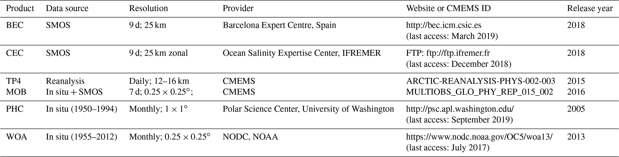
Recently two gridded sea surface salinity (SSS) products that cover the Arctic Ocean have been derived from the European Space Agency (ESA)'s Soil Moisture and Ocean Salinity (SMOS) mission: one developed by the Barcelona Expert Centre (BEC) and the other developed by the Ocean Salinity Expertise Center of the Centre Aval de Traitement des Données SMOS at IFREMER (The French Research Institute for Exploitation of the Sea) (CEC). The uncertainties of these two SSS products are quantified during the period of 2011–2013 against other SSS products: one data assimilative regional reanalysis; one data-driven reprocessing in the framework of the Copernicus Marine Environment Monitoring Services (CMEMS); two climatologies – the 2013 World Ocean Atlas (WOA) and the Polar science center Hydrographic Climatology (PHC); and in situ datasets, both assimilated and independent. The CMEMS reanalysis comes from the TOPAZ4 system, which assimilates a large set of ocean and sea-ice observations using an ensemble Kalman filter (EnKF). Another CMEMS product is the Multi-OBservations reprocessing (MOB), a multivariate objective analysis combining in situ data with satellite SSS. The monthly root mean squared deviations (RMSD) of both SMOS products, compared to the TOPAZ4 reanalysis, reach 1.5 psu in the Arctic summer, while in the winter months the BEC SSS is closer to TOPAZ4 with a deviation of 0.5 psu. The comparison of CEC satellite SSS against in situ data shows Atlantic Water that is too fresh in the Barents Sea, the Nordic Seas, and in the northern North Atlantic Ocean, consistent with the abnormally fresh deviations from TOPAZ4. When compared to independent in situ data in the Beaufort Sea, the BEC product shows the smallest bias (< 0.1 psu) in summer and the smallest RMSD (1.8 psu). The results also show that all six SSS products share a common challenge: representing freshwater masses (< 24 psu) in the central Arctic. Along the Norwegian coast and at the southwestern coast of Greenland, the BEC SSS shows smaller errors than TOPAZ4 and indicates the potential value of assimilating the satellite-derived salinity in this system.


The sea surface salinity (SSS) plays a key role in tracking processes in the global water cycle through precipitation, evaporation, runoff, and sea-ice thermodynamics (Vialard and Delecluse, 1998; Sumner and Belaineh, 2005; Vancoppenolle et al., 2009; Yu, 2011). SSS is known to impact the oceanic upper mixing significantly (Latif et al., 2000; de Boyer Montegut et al., 2004; Maes et al., 2006; Furue et al., 2018) via its effect on the surface layer density (Johnson et al., 2012). The SSS also affects the decadal variability of hydrography in the upper waters of the North Atlantic (Reverdin et al., 1997). Using a coupled atmosphere–ocean model and an observed SSS climatology dataset, Mignot and Frankignoul (2003) attributed the interannual variability of the Atlantic SSS to two factors: anomalous Ekman advection and the freshwater flux. Additionally, the increased melting of glaciers and sea ice in the Arctic (McPhee et al., 1998; Macdonald et al., 1999) leads to significant changes in the salinity distribution and freshwater pathways (Steele and Ermold, 2004; Morison et al., 2012). The freshwater flux is regarded as one of the least constrained parameters in ocean models due to poorly known river discharge, precipitation, and glacial or sea-ice melt (e.g., Tseng et al., 2016; Furue et al., 2018). In ocean models the sea surface freshwater flux is often adjusted directly or the SSS is restored to its corresponding climatological value to avoid salinity drift.
Monitoring SSS from space is crucial for understanding the global water cycle and the ocean dynamics, especially in the Arctic Ocean where our knowledge of the SSS variability is limited due to nonhomogeneous and sparse in situ data. The European Space Agency's (ESA) Soil Moisture and Ocean Salinity (SMOS) satellite, launched in November 2009, consists of the Microwave Imaging Radiometer using Aperture Synthesis (MIRAS), a passive 2-D interferometric radiometer operating in L band (1.4 GHz, 21 cm), that measures the brightness temperature (BT) emitted from the Earth. The L-band microwave is highly sensitive to water salinity, which influences the dielectric constants in the sea, and is less susceptible to atmospheric or vegetation-induced attenuation than higher-frequency measurements (Font et al., 2010; Kerr et al., 2010; Mecklenburg et al., 2012). Committed to providing global salinities averaged over 10–30 d with an accuracy of 0.1 psu in the open ocean, ESA provides the MIRAS data in SMOS Level 1 (L1) and Level 2 (L2) products through a set of sequential processors (Mecklenburg et al., 2012; ESA, 2017).
Over the ocean, Level 2 products (L2OS) are comprised of three different ocean salinities, together with the BTs at the top of atmosphere and at the sea surface, distributed by ESA in a swath-based format (e.g., SMOS Team, 2016; ESA, 2017). As a result of the efforts of the national agencies in France and Spain, two Level 3 (L3) data products of SSS are freely available, which are independently developed by the Ocean Salinity Expertise Center of the Centre Aval de Traitement des Données SMOS at The French Research Institute for Exploitation of the Sea (IFREMER) and the Barcelona Expert Centre. These two SMOS products have successfully resolved the Agulhas salinity front (D'Addezio et al., 2016) and proven useful for estimating precipitation (Supply et al., 2018). The work of Olmedo et al. (2018) quantitatively evaluates the accuracy of the SMOS Arctic and sub-Arctic SSS to less than 0.35 psu, but this evaluation against Argo data was limited by the lack of data in the Arctic proper. The present study thus investigates the accuracy of these two L3 SSS products from SMOS in the Arctic Ocean.
A good estimate of surface salinity is a necessary step towards knowledge of the three-dimensional water mass properties, for which data assimilation and optimal interpolation methods must be invoked. In a recent study, Uotila et al. (2019) investigated the Arctic salinity in 10 ocean reanalysis products and found disagreements within them regarding the seasonal cycle in the upper layer (0–100 m; Fig. 12 of Uotila et al., 2019). Although most reanalysis products (7 out of 10 reanalyses in Table 1 of Uotila et al., 2019) restored salinity to climatology, they did not use the same salinity climatology, which betrays the lack of a universal SSS reference. Note that the full assessment of the Arctic SSS products has been hindered by the extreme paucity of in situ data in the Arctic. The SSS data from the SMOS mission should in principle allow the evaluation of salinity on a basin scale. In this study, we use two SSS products available from the Copernicus Marine Environment Monitoring Service (CMEMS). The first is the regional Arctic CMEMS reanalysis (ARCTIC-REANALYSIS-PHYS-002-003) from the TOPAZ4 assimilation system, which is a coupled ocean and sea-ice data assimilation system using the ensemble Kalman filter (EnKF) to assimilate the various ocean and sea-ice observations (e.g., Xie et al., 2017). This is an official physical multi-year CMEMS product for the Arctic region, which has been extended yearly by the Arctic Marine Forecasting Center (MFC). The second is the CMEMS multivariate optimal interpolation reprocessing (MULTIOBS_GLO_PHY_REP_015_002, Droghei et al., 2018). The latter product directly merges in situ data with satellite measurements including SMOS without the use of a model and is therefore a reprocessing rather than a reanalysis. There are four other global reanalysis products under CMEMS, but understanding their differences well requires an intimate knowledge of their setup and is beyond the scope of the present study.
We assess the quantitative deviations of Arctic SSS among the two SMOS products and the two CMEMS products, together with two climatology datasets: WOA13 (version 2.0 of World Ocean Atlas of 2013; Zweng et al., 2013) and the older PHC (Polar Science Center Hydrographic Climatology version 3.0; Steele et al., 2001). We further extend the evaluation using available in situ salinity observations during the years 2011–2013 from different data sources. Can the evaluation against in situ data also shed light on the uncertainties of the SMOS products? Can it also give useful information needed for the assimilation of the SMOS SSS products into an Arctic ocean forecast–reanalysis system?
The paper is organized as follows: Sect. 2 describes all SSS products and the in situ datasets. The monthly mean SSS from these six products are intercompared and monthly differences from the TOPAZ SSSs are analyzed in Sect. 3. Section 4 evaluates the SSS products against in situ data, which are divided between assimilated and independent data. A summary of this study is provided in Sect. 5.
2.1 Sea surface salinity from SMOS
The SSS retrieval from SMOS is subject to biases originating from various non-geophysical sources such as the so-called land–sea contamination and the latitudinal biases, mainly caused by the thermal drift of the instrument. A particular challenge in the Arctic is the sea-ice edge because of ice–ocean contamination. Based on different statistical approaches, matchup criteria, and SMOS data filtering flags, two centers have developed separate processing chains producing a Level 3 SSS product on a regular grid. These two SSS products are hereafter named CEC and BEC, respectively, in this study, evaluated during the 3 years of 2011–2013 (see Table 1).
Table 1Details of the six products evaluated during 2011–2013.
2.1.1 The BEC product
The latest regional Arctic product (version 2.0) from BEC is available from http://bec.icm.csic.es (last access: March 2019) for the period since December 2018. The BEC SSS product was generated from ESA L1B (v620) products and accumulates salinity data over 9 d with a spatial grid resolution of 25 km. With respect to its previous version, a systematic bias in the retrieved salinity is corrected by computing the SMOS climatology (the most probable value for a given lat–long, incidence angle and across-swath distance), which is substituted by a reference value from WOA13. In addition, a temporal bias correction has been refined in this version using near-surface Argo salinity to compute regional averages (see the details in Olmedo et al., 2018).
2.1.2 The CEC product
The third version of LOCEAN SMOS SSS L3 maps (L3_DEBIAS_LOCEAN_v3) was released by the Ocean Salinity Expertise Center at IFREMER in July 2018. Every 4 d, the SSS maps averaged over 9 d are released on ftp://ftp.ifremer.fr (last access: December 2018). This product uses the Equal-Area Scalable Earth Grid (EASE-Grid) which has limited grid distortion and a spatial resolution of 25 km. Using a Bayesian retrieval approach (Kolodzejczyk et al., 2016), the SMOS systematic errors in the vicinity of continents are discarded to improve the product quality. Further, a “de-biasing” method (Boutin et al., 2018) has been applied in this version of the CEC product, in which the non-Gaussian distribution of SSS is taken into account, refining the latitudinal correction at high latitude and preserving the naturally seasonal variability of SSS.
2.2 Sea surface salinity from two CMEMS products
2.2.1 The TOPAZ4 Arctic MFC reanalysis
TOPAZ4 uses version 2.2 of the Hybrid Coordinate Ocean Model (HYCOM; Chassignet et al., 2003; Bertino and Lisæter, 2008) coupled with a simple thermodynamic sea-ice model (Drange and Simonsen, 1996) in which the elastic–viscous–plastic rheology describes the sea-ice dynamics (Hunke and Dukowicz, 1997). The model domain covers the Arctic Ocean and the North Atlantic Ocean with a horizontal resolution of 12–16 km. In order to obtain an accurate and dynamically consistent reanalysis in the Arctic Ocean, the deterministic EnKF (DEnKF; Sakov and Oke, 2008) was implemented in TOPAZ with a dynamical ensemble of 100 members all driven by perturbed 6-hourly atmosphere forcing from ERA interim (Simmons et al., 2007). The perturbations of precipitation events follow a log-normal probability distribution and conserve the ensemble-average total precipitation.
Along the model lateral boundaries in the South Atlantic and in the Bering Strait, temperature and salinity are relaxed to combined climatology data from PHC and WOA. The river discharges are treated as an additional mass and a negative salinity flux. Near the surface, to avoid the salinity drift (Tseng et al., 2016; Furue et al., 2018), a weak relaxation to the same combined climatological SSS with 30 d decay is used as in most ocean models, but it is restricted to the areas where the difference to climatology is smaller than 0.5 psu. The EnKF assimilates various ocean and sea-ice observations (e.g., Xie et al., 2016, 2018) into a multivariate state update of the HYCOM model.
The understanding for the uncertainty of the TOPAZ4 SSS has been hindered by poor coverage of in situ data over the Arctic domain, although Xie et al. (2017) had comprehensively assessed the TOPAZ4 reanalysis during 1991–2013 against various types of ocean and sea-ice observations. For the sake of brevity, the TOPAZ4 reanalysis SSS is named TP4 hereafter.
2.2.2 SSS from the Multi-OBservations dataset
The CMEMS product of MULTIOBS_GLO_PHY_REP_015_002 combines the SSS observations from in situ and satellite data, using optimal interpolation (OI; Buongiorno Nardelli et al., 2016; Verbrugge et al., 2018) at a weekly interval on a 0.25∘ × 0.25∘ regular grid. The main datasets used during the OI processing are (1) the quality-controlled in situ data from the COriolis dataset for Re-Analysis (CORA; Cabanes et al., 2013) distributed through CMEMS; (2) the objectively analyzed SSS and sea surface temperature (SST) data generated from CORA, also distributed by CMEMS, which uses the WOA climatology as a first guess and has been upscaled to the Multi-OBservations reprocessing (MOB) grid as another first guess of the multidimensional OI; (3) the SMOS L3 binned (L3bin) data reprocessed by SMOS-BEC on a 0.25∘ grid, despite the previous version 1.0 of the product mentioned above; (4) the daily Reynolds L4 AVHRR_OI Global blended SST product on a 0.25∘ grid. This product is called MOB hereafter.
2.3 Surface salinity from in situ data
The in situ SSS data are acquired here from three quality-controlled datasets. The first data source is CORA from CMEMS (product ID: INSITU_GLO_TS_REP_OBSERVATIONS_013_001_b), also used in the MOB SSS. CORA contains temperature and salinity profiles from various in situ data sources (Cabanes et al., 2013). Since 2013, the CORA dataset has been updated every year and includes all the Argo float profiles, moorings, gliders, ice-tethered profilers (ITPs; Toole et al., 2011), expendable bathythermograph (XBT), conductivity–temperature–depth (CTD), and expendable conductivity–temperature–depth(XCTD) data. The latest version of the dataset, CORA5.1, covers the period of 1950–2016. Figure 1a shows the distribution of SSS (averaged over 0–8 m depth) observations from CORA5.1 (total 69 246 observations) over the domain north of 52∘ N during the years 2011–2013.

Figure 1(a) SSS locations of the in situ observations north of 52∘ N in CORA5.1 during the years 2011–2013. Eight sub-regions divide the Arctic Ocean (S0–S4) and the northern North Atlantic Ocean (S5–S7), with the number of observations indicated in each region. (b) Independent SSS observations in the Beaufort Sea during the summer months of 2011–2013 from the BGEP (marked by inverted triangles, squares, and stars) and the CLIVAR (marked by triangles and crosses). Different colors (red, black, and yellow) indicate the years (2011, 2012, and 2013, respectively).
The second source of in situ data is from the Beaufort Gyre Experiment Project (BGEP; http://www.whoi.edu/website/beaufortgyre/background, last access: 14 December 2018). In order to monitor the natural variabilities of the Beaufort Sea in the Canada Basin, BGEP has maintained moorings since 2003 and acquires in situ measurements over the Beaufort Sea region every summer. The symbols (inverted triangle, square, and star) shown in Fig. 1b indicate the locations of valid SSS observations obtained from BGEP. The in situ dataset used in this study is obtained from the GO-SHIP (the Global Ocean Ship-based Hydrographic Investigations Program; Talley et al., 2017) database under the Climate Variability and Predictability Experiment (CLIVAR). The SSS observations in the Beaufort Sea are extracted from CLIVAR/GO-SHIP data with EXPOCODE (33HQ20111003 and 33HQ20121005, Mathis and Monacci, 2014), which are available from https://cdiac.ess-dive.lbl.gov/ftp/oceans/CARINA/Healy/ (last access: 18 December 2018). All the valid salinity profiles are averaged within the upper 8 m layer, in order to achieve the best match with the satellite SSS measurements. Contrary to the CORA data, both BGEP and CLIVAR data are independent from all the evaluated datasets.
Prior to the intercomparison of different SSS products, all the gridded products from satellite, reanalysis, and climatology have been mapped onto the same grid used in the TP4 model by a “nearest-neighbor” interpolation. To quantitatively evaluate the SSS deviation in the Arctic, the bias and the root mean square deviation (RMSD) are defined by
where p is the length of the time series, is the valid salinity from different sources at the ith time, compared to the reference salinity field si. Hi is the observation operator projecting onto si.
3.1 Monthly mean comparison of SSS
Figure 2 shows the monthly mean Arctic SSS in March from the six products. Notable differences in the two SMOS products appear in the Nordic Seas, Barents Sea, and around the Labrador Sea. At first sight, the large-scale SSS features from SMOS products are similar to the other products. However, the CEC SSS is fresher (as shown by the isolines of 35 psu) compared to the BEC, TP4, MOB, and both climatologies. The location of the sea-ice edge in the two SMOS products matches comparatively well with the TP4 reanalysis (Fig. 2a, d). In the sea-ice-covered region, TP4 shows a gradual decrease in SSS from the European to the American sector, with two minima near the Beaufort Sea and the East Siberian Sea (ESS; Fig. 2b) consistent with the PHC (Fig. 2c). Those are unclear in MOB and WOA (Fig. 2e, f), especially the SSS minimum in the Beaufort Sea. The latter two products also show artificial projection artifacts around the North Pole.
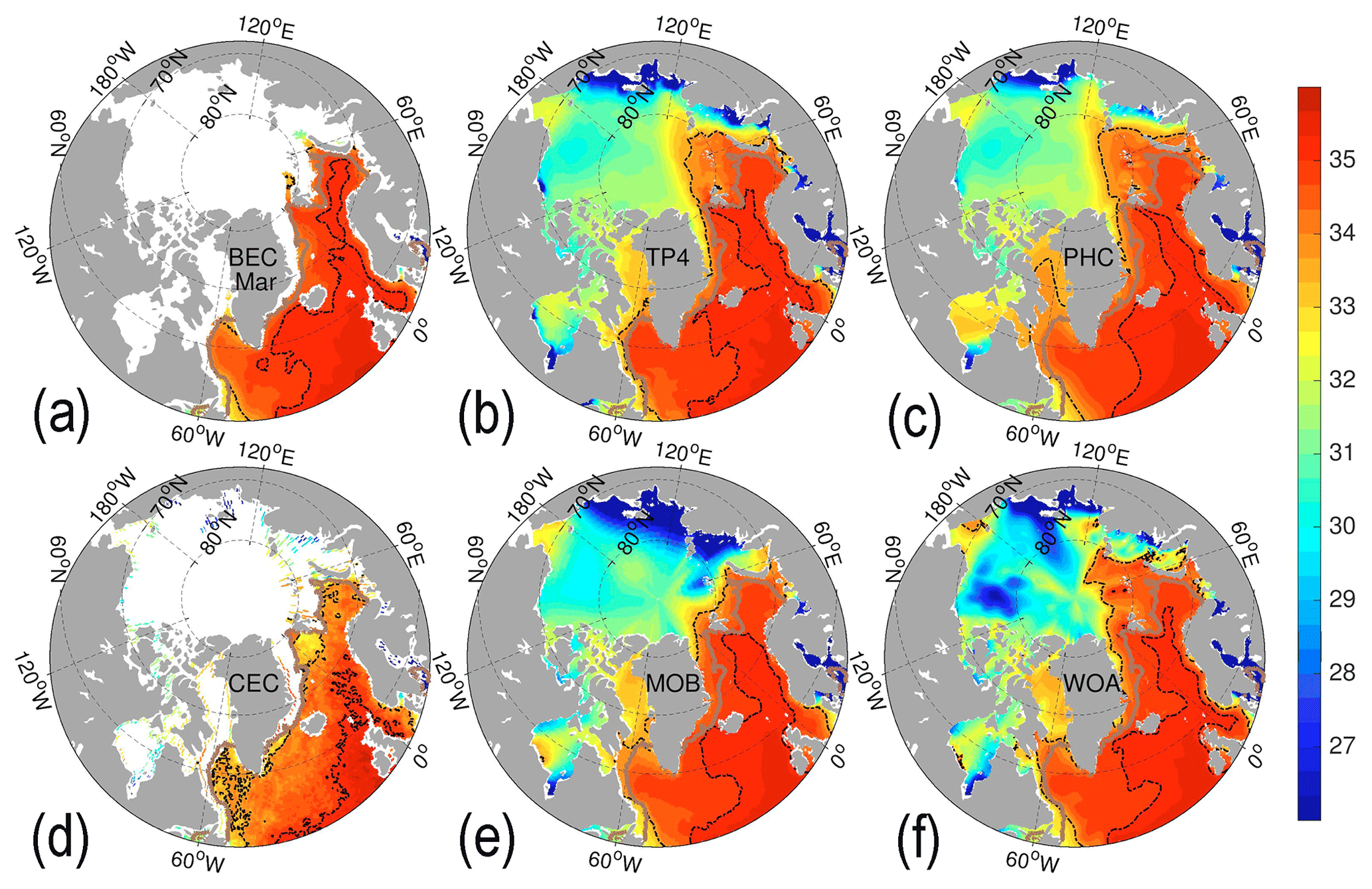
Figure 2Monthly SSSs (unit: psu) in March from satellite products (BEC and CEC, a, d), reanalysis or reprocessing (TP4 and MOB, b, e), and climatology (PHC and WOA, c, f). White areas are masked by sea ice. The thick brown line represents the sea-ice edge (15 % concentration from TP4), and the black shaded isolines represent the salinities of 33.6 and 35 psu near the surface.
Figure 3 shows the corresponding SSS fields in September. In comparison to the March situation, the BEC and CEC SSS in the Nordic Seas are both less saline, indicated by the 35 psu isoline. The sea-ice masking of the two SMOS products differs considerably in the Canadian Basin and in the Arctic marginal seas. Although the SSS of TP4, MOB, PHC, and WOA agree relatively well in the North Atlantic Ocean as shown by the dashed lines of 35 psu, the discrepancies become dramatic in ice-covered areas. Below the ice or near the sea-ice edge (denoted by the thick brown line in Figs. 2 and 3), TP4 and PHC share common features, which can be explained by the model restoring itself to PHC. On the other hand, MOB and WOA differ significantly in spite of WOA being used as input to MOB. Short of a universal reference for Arctic SSS, the monthly mean SSS deviations will be quantified using TP4 as a reference.
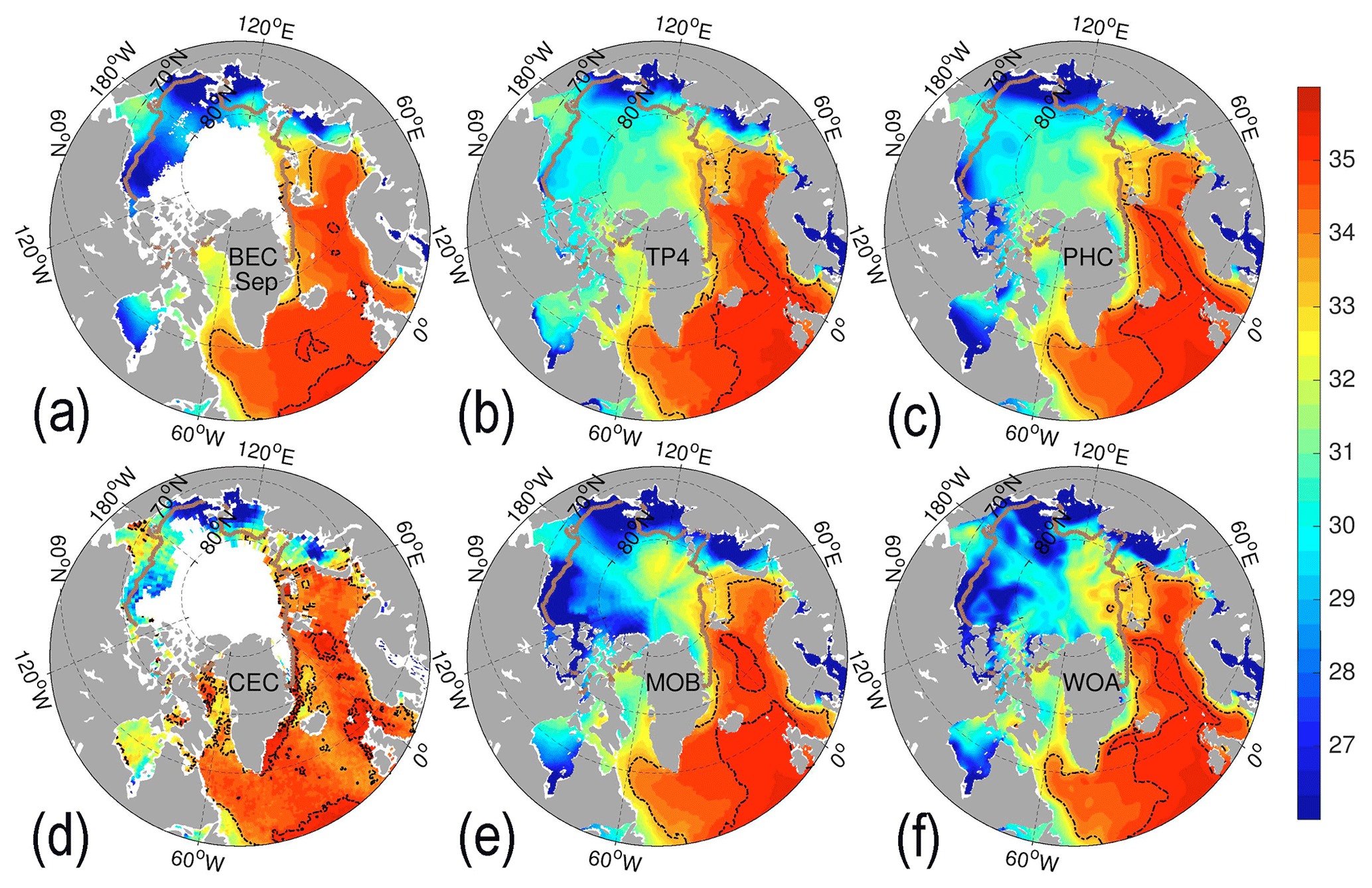
Figure 3Similar to previous figure but for September.
3.2 Deviation analysis of monthly SSS referenced to TP4
Figures 4 and 5 show the deviations of the monthly mean SSS of the five products with reference to the TP4 SSS in August and September, respectively. In August, the two SMOS products (Fig. 4a, c) show coherently negative deviations (∼2 psu) in the marginal seas of the Beaufort Sea, the ESS, the Laptev Sea, and the Kara Sea. A positive deviation of CEC is noticeable in the Kara Sea, which indicates that the land–ocean interaction is stronger than in BEC. In the North Atlantic Ocean, away from the sea-ice edge, the deviation of the BEC from TP4 is lower (bias less than 0.5 psu). Focusing on the Arctic domain (> 60∘ N), the mean deviation of the BEC SSS is −0.87 psu and its root mean square is 1.75 psu. The CEC SSS shows considerable negative deviations over 1 psu in the North Atlantic, from north of Denmark Strait to the west coast of Ireland. This is remarkably different from the BEC and does not discern the subpolar from the subtropical waters there (Hátún et al., 2005). For the BEC and CEC products that use different ice masks, the deviations are averaged outside their respective ice mask, not their intersection. Comparing the low-salinity lines of 33.6 psu in Fig. 3a and d, it clearly shows the polar water southward of Arctic has a misinterpretation in CEC owing to the ice mask used. The deviations of MOB and the two climatology products are comparatively small in the open ocean of the North Atlantic (Fig. 4b, e). Near and below the sea-ice cover reproduced by TP4 (the thick brown line in the figures), the deviations are much larger, particularly both MOB and WOA show strong saline anomalies (> 1 psu) in the Eurasian Basin and low anomalies in the Amerasian Basin.
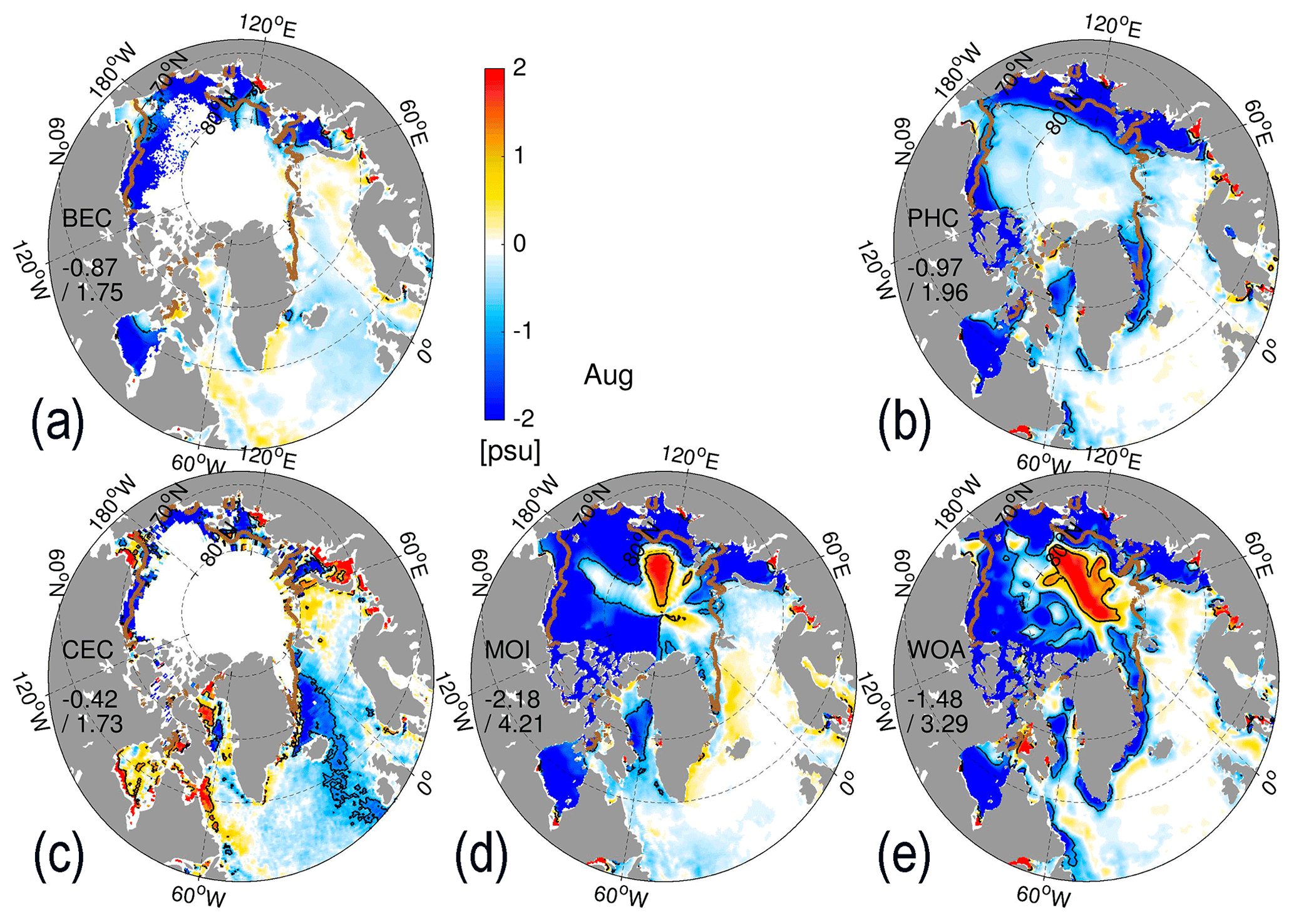
Figure 4Deviations of monthly SSS (unit: psu) in August for (a) BEC, (b) PHC, (c) CEC, (d) MOB, and (e) WOA relative to TP4. The thick brown line represents sea-ice edge (15 % concentration from TP4), the black lines represent ±1 psu.

Figure 5Same as previous figure but for September.
In September, the SSS deviations of BEC, MOB, PHC, and WOA show similar fresher patterns as in August, but the CEC deviations becomes surprisingly positive around the ice edge. The SSS deviation of CEC, averaged over the Arctic domain (> 60∘ N), changes from −0.42 to 0.42 psu from one month to the next one. The seasonal evolution of monthly SSS deviations from TP4 for all five remaining products, averaged over the Arctic, is shown in Fig. 6. Among the five products, MOB shows the strongest seasonality with the RMSD and is higher than 4 psu in July and August (Fig. 6a) and close to 2 psu in winter. The spatially averaged deviation is much fresher than TP4: over −2 psu in summer and −0.5 psu in winter (Fig. 6b). The deviations of the two SMOS SSS show a relatively smaller seasonality (Fig. 6a). During the summer months, their RMSDs reach 1.5 psu (Fig. 6a), and they decrease to 0.5 and 1.0 psu (for BEC and CEC, respectively). Throughout the whole year, the BEC RMSDs (Fig. 6a) are consistently smaller than that of CEC, and the seasonal cycles are different. This shows that the BEC SSS is closest to TP4, although it is overall fresher in the summer.
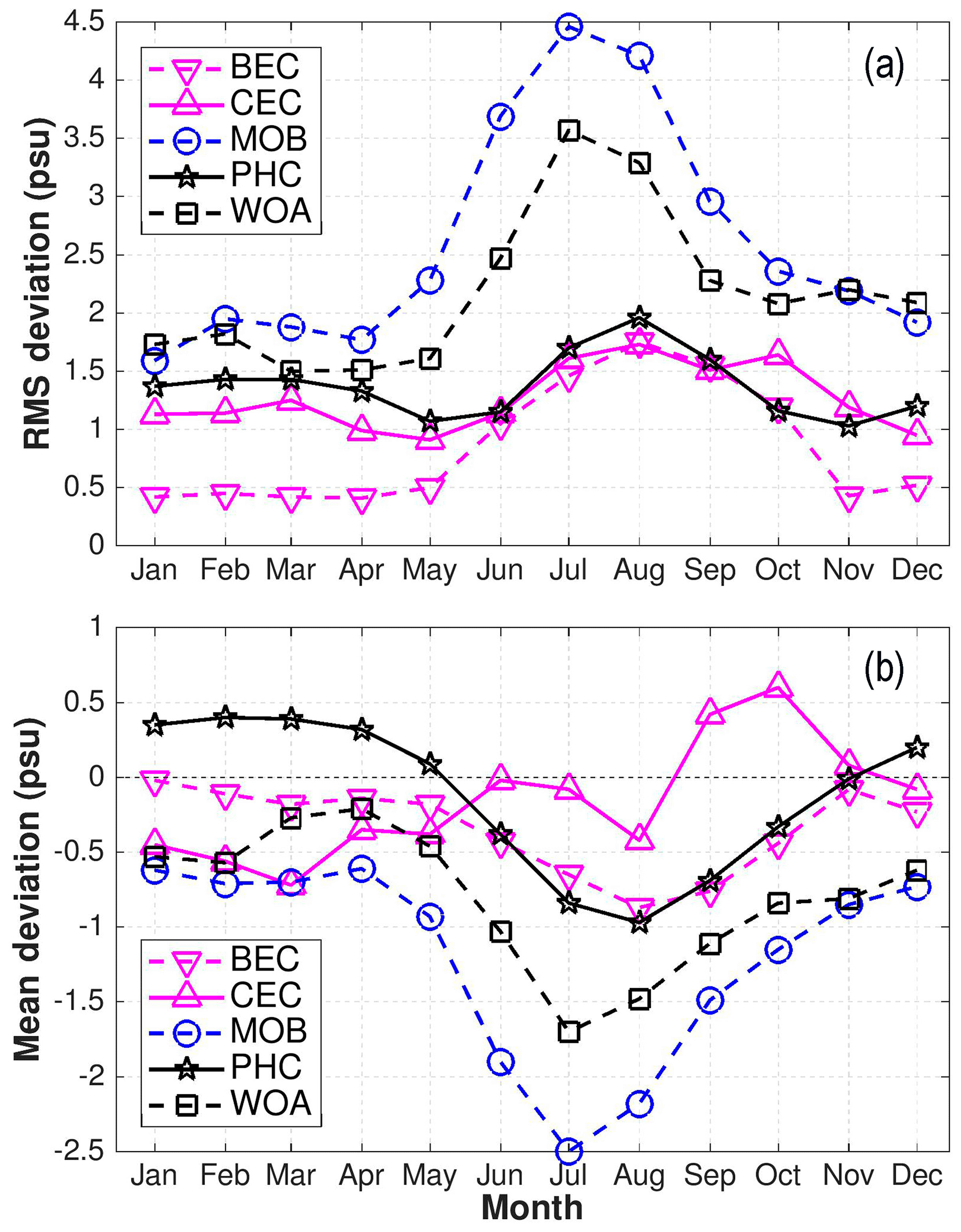
Figure 6Monthly deviations in the Arctic Ocean (> 60∘ N) of (a) the rms and (b) the spatial average during the period 2011–2013 for the five SSS products referenced to TP4. The lines with inverted triangle, triangle, circle, star, and square represent the SSS deviations from BEC, CEC, MOB, PHC, and WOA, respectively.
The misfits of the six SSS products from SMOS, CMEMS, and climatologies are calculated as in Eqs. (1) and (2) against the point-wise in situ observations described in Sect. 2.3. For TP4, the SSS evaluation is conducted on the same model day as the in situ observations. Owing to the fact that the SSSs from BEC, CEC, and MOB are averaged over either 9 d or 1 week (see Table 1), the product dates at the center of the averaging window lag behind 5 or 4 d compared to the observation date. For PHC and WOA, the in situ observations are sorted to monthly bins and evaluated for each month. The quantitative evaluation is divided into two main sections starting with dependent and then independent observations.
4.1 Against SSS from CORA5.1
As shown in Fig. 1a, the distribution of SSS observations from CORA5.1 over the Arctic is very inhomogeneous during the 3 years. Due to this, the evaluation of the gridded SSS products against in situ observations is restricted to the observation-rich regions. The SSS misfits bias and RMSD for the six products are reported in Table 2 according to the eight Arctic sub-regions defined previously (Fig. 1a). In this study, the Arctic domain (> 60∘ N) is the core region for evaluation, divided into five sub-regions numbered from S0 to S4. It contains the central Arctic (sub-regions S0, S1, S2, and S3) and the Nordic Seas (S4). The regions from S5 to S7 are in the northern North Atlantic. The observations are displayed on scatterplots (Figs. 7 and 8) to exhibit their uncertainties for fresh and saline waters in different areas.
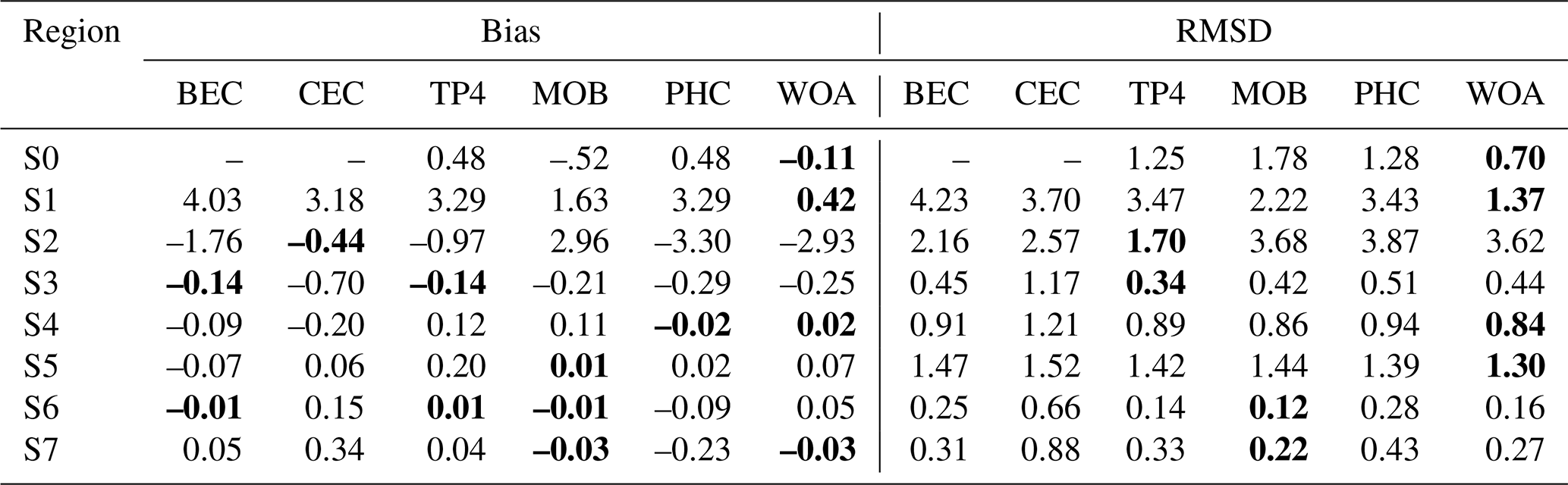
Table 2Misfits of SSS (unit: psu) relative to in situ observations (CORA5.1) during 2011–2013 in each sub-region. Bold numbers denote the smallest error among the six products.
4.1.1 Central Arctic
Figure 7 shows the SSS products compared with discrete observations in the central Arctic. The observed SSS in S0 and S1 are mainly from the ITP at a minimal depth of 8 m. Around the North Pole (S0), where the satellite SSSs are absent, the TP4 reanalysis and MOB reprocessing show opposite biases: +0.48 and −0.52 psu, respectively (Table 2). The two climatologies used by them, PHC and WOA, respectively, also show opposite biases. Considering the latter climatologies, both SSS scatterplots shows a fresh bias for high-salinity water (> 33 psu) and a saline bias for low-salinity water (< 31 psu).
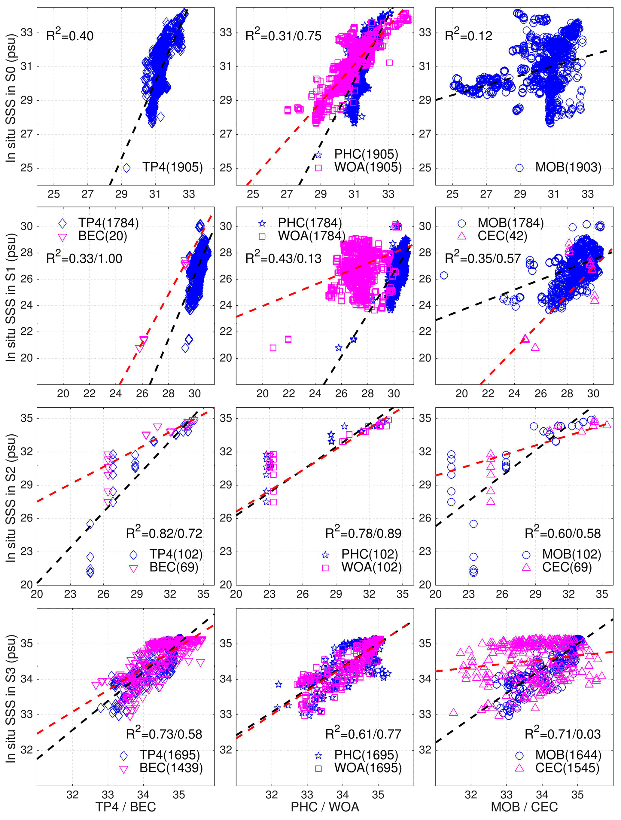
Figure 7Scatterplots of SSS compared to the CORA5.1 in situ observations with respect to the S0–S3 regions in the Arctic. The diamonds, inverted triangles, stars, squares, circles, and triangles represent the SSS from TP4, BEC, PHC, WOA, MOB, and CEC, respectively. The black (red) lines are the linear regressions of the blue (purple) dots in each panel, and the coefficient R2 between the evaluated product and the in situ SSS is indicated in the panels together with the number of observations in parentheses.
In the Canadian Basin (in S1), the two climatological SSSs show an obvious gap in comparison to the ITP observations. Comparing to the fresh in situ SSS from 24 to 30 psu, the PHC has a strong saline bias (from 2 to more than 5 psu). On the other hand, the WOA shows both a fresh bias for relatively high-salinity water (> 28 psu) and a saline bias for fresher water (< 26 psu). Owing to the different time periods (Table 1) of the in situ data they used, this result confirms the freshening of the Canadian Basin since the 1990s (Morison et al., 2012).
In the S1 sub-region, the satellite SSSs from BEC and CEC only have 20 and 42 data points for evaluation, respectively. The resulting scatterplots show a significantly positive salinity bias (> 4 psu) for fresh waters (< 27 psu). For relatively higher-salinity water (> 27 psu), the CEC has a stronger saline bias than the BEC.
In the Kara Sea (sub-region S2), the TP4 SSS has the smallest RMSD at 1.7 psu, which is significantly smaller than other products. The scatterplot also shows a good linear relationship between the TP4 and the in situ SSS, while other products generally show fresh biases, indicating that the SSS variability in the Kara Sea is well captured by TP4. In the Barents Sea (sub-region S3), TP4 also gives the smallest misfit (RMSD: 0.34 psu; bias: −0.14 psu). The SSS scatterplots exhibits linear relationships for all products except the CEC, which underestimates the Atlantic water SSS.
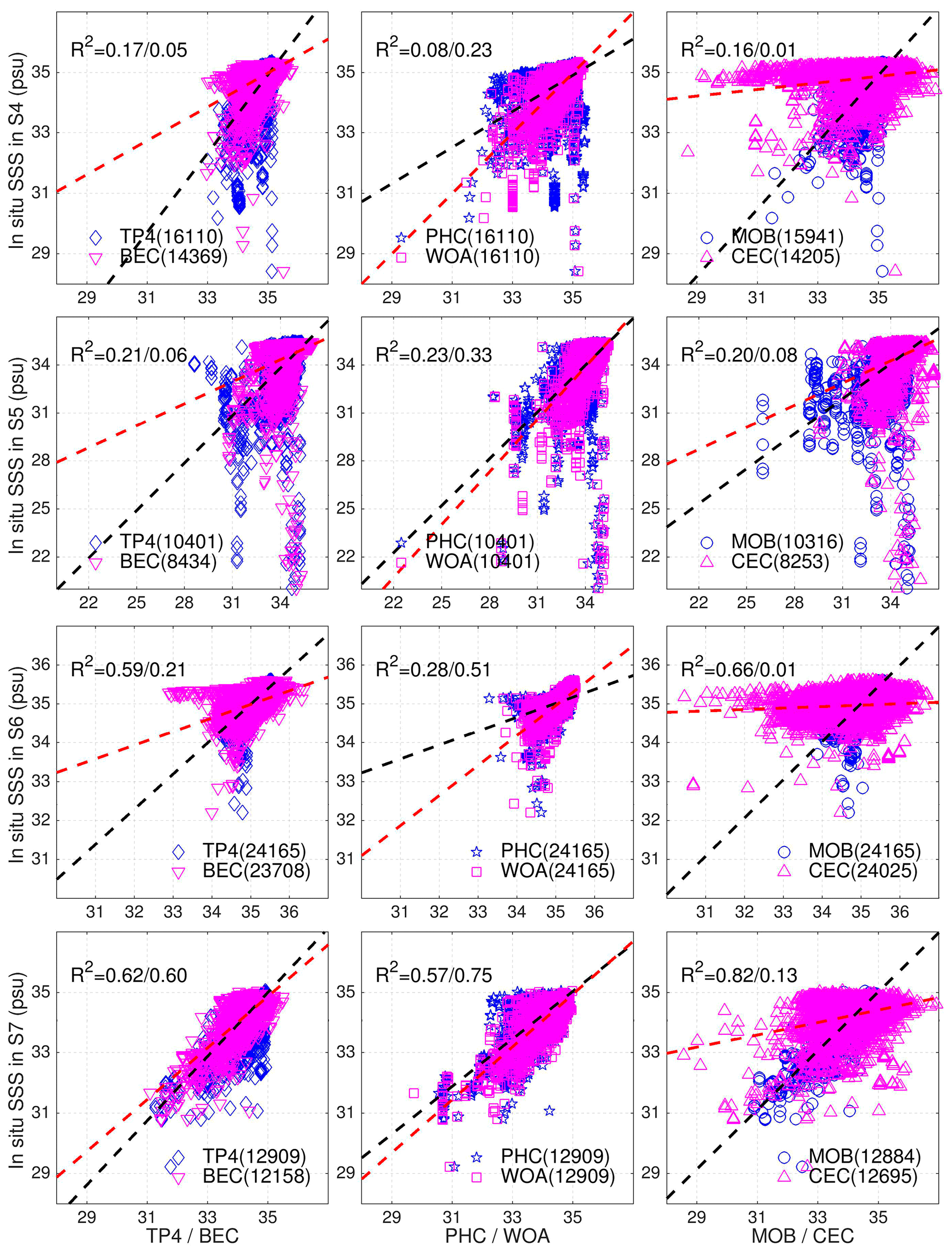
4.1.2 Northern North Atlantic and Nordic Seas
Figure 8 shows the paired scatterplots of the six SSS products in the subpolar seas from sub-regions S4 to S7 (see Fig. 1a). In S4 and S5, the bias of SSS products is relatively small (less than 0.15 psu) (Table 2), except for CEC in S4 and TP4 in S5, both too saline by 0.2 psu. The scatterplots further indicate that low-salinity waters are too saline in all SSS products in S4 (< 31 psu) and in S5 (< 28 psu). Meanwhile, the respective bias and RMSD of the SSS products are less than 0.1 and 0.43 psu except for the CEC in S6 and S7. The MOB SSS has the smallest salinity bias. Among the eight regions compared here (S0 to S7), the SSS bias is lowest in S6 (Irminger Sea).
Over the northern North Atlantic and the Nordic Seas, Fig. 9 shows maps of the mean SSS deviation for each product during the period 2011–2013. Considerable negative biases (< −0.2 psu) are found in the CEC, whereas MOB and WOA have the smallest bias: less than 0.02 psu (Fig. 9d, e, f). The SSS products from BEC, TP4, and PHC (Fig. 9a, b, c) have a slightly higher bias (∼0.05 psu) in comparison to MOB and WOA. On average, the BEC bias is only −0.04 psu, much smaller than that of the CEC (< −0.2 psu). Focusing on the BEC SSS, Fig. 9a shows that while a fresh bias dominates the Nordic Seas, the product is too saline in the northern North Atlantic.

Figure 9The mean deviation of SSS for the six datasets compared to in situ observations from CORA 5.1 during the 3 years of 2011–2013 in the northern North Atlantic and the Nordic Seas. The SSS observations are distributed across the coarse grid cells of 9×9 grids in TP4, with a gray mask if the valid observations are fewer than 10.
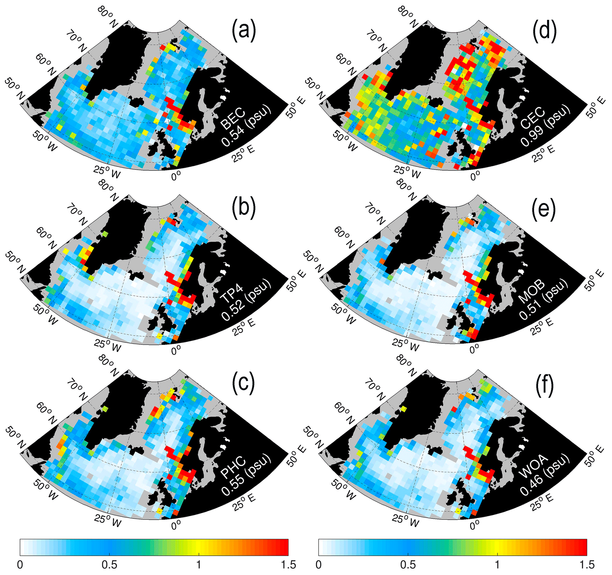
Figure 10The root mean square deviation of SSS for six datasets compared to in situ observations from CORA 5.1 during the 3 years of 2011–2013 in the northern North Atlantic and the Nordic Seas. The SSS observations are distributed across the coarse grid cells of 9×9 grids in TP4, with a gray mask if the valid observations are fewer than 10.
The intercomparison of the biases against the in situ data in Fig. 9a and b exhibits two strong positive biases of TP4 along the Norwegian coast and along the west Greenland coast. Notably, the BEC has a smaller bias along both coasts, although it has a slightly saline bias offshore. This indicates potential benefits of the BEC SSS for the TOPAZ system along the Norwegian and Greenland coasts, were it successfully assimilated into the system. Figure 10 shows RMSDs of SSS for all the products over the northern North Atlantic Ocean and the Nordic Seas. On average, the largest uncertainty is found with the CEC (∼1.0 psu; Fig. 10d), with RMSDs as large as 1.5 psu in the Greenland Sea and the Barents Sea. The SSS RMSDs for the five other SSS products are much smaller (∼0.5 psu).
4.2 Independent SSS in the Beaufort Sea
Independent in situ data from BGEP and CLIVAR are used during the summer months of 2011–2013 in the Beaufort Sea for the evaluation of the six SSS products (Fig. 11). The in situ SSS observations range from 15 to 32 psu. The range of BEC SSS is limited to 24 to 31 psu with a minor bias of 0.09 psu and an RMSD of 1.82 psu. On the other hand, the range of TP4 SSS increases from 19 to 32 psu, with a larger saline bias of 2.59 psu and an RMSD of 3.63 psu. The linear regression coefficients for BEC and TP4 are 0.57 and 0.07, respectively. Looking at the low-salinity observations (∼ 27 psu) collected at (136.4∘ W, 70.5∘ N) on 15 August 2011, marked by inverted triangles (Fig. 1b) near the Mackenzie River estuary, TP4 has a significant negative bias (< −4 psu) visible as the outliers above the dashed black line in Fig. 11a. This hints at a lack of freshwater signatures from river discharge.
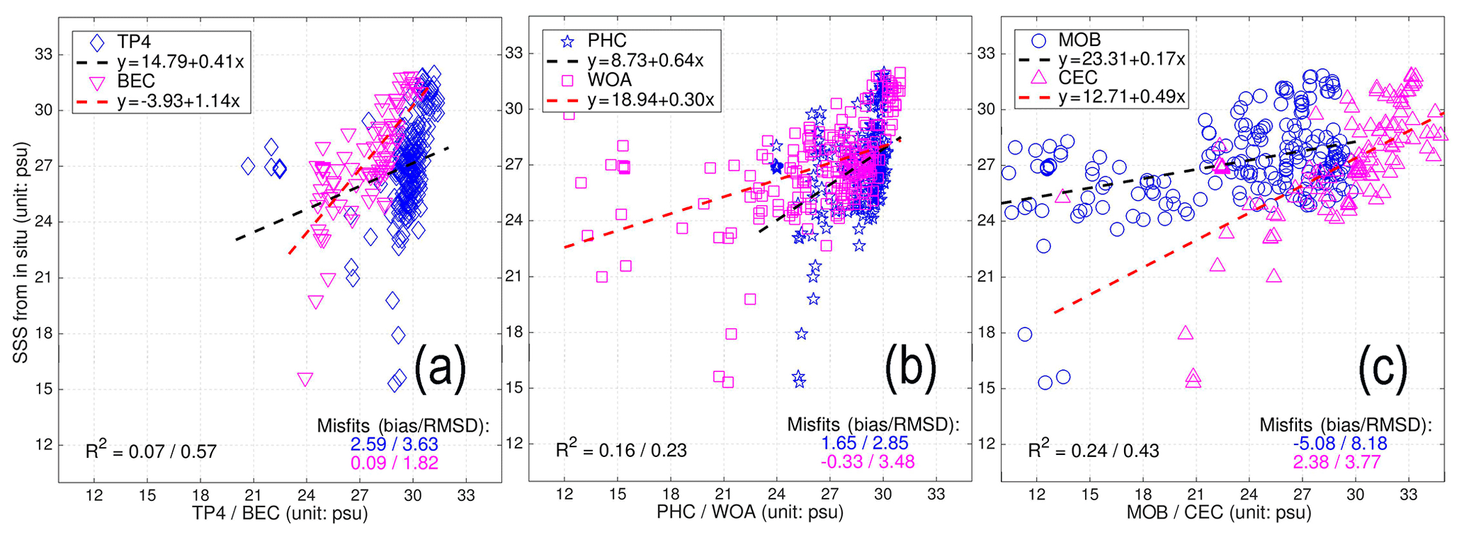
Figure 11Scatterplots of SSS compared to the in situ observations in the Beaufort Sea during the summer months of 2011–2013. (a) The diamond (inverted triangle) represents the SSS from TP4 (BEC) with blue (purple), and the linear regression is denoted by the dashed black (red) line. (b) The star (square) from the climatology of PHC (WOA). (c) The circle (triangle) represents from MOB (CEC). The coefficient R2 is the squared linear relationship between the evaluated product and the in situ SSS, and the misfits are also shown on the panels.
The range of PHC SSS climatology only reaches from 24 to 31 psu, similar to TP4, with a saline bias of 1.65 psu and RMSD of 2.85 psu. Compared to the TP4 deviation at the Mackenzie River basin, the PHC saline bias is present but smaller. The strong positive bias in TP4 at these points can then be partly attributed to the SSS relaxation of the TOPAZ model towards the PHC climatology, albeit a rather weak relaxation. The range of the WOA is much wider: from 12 to 31 psu. Among the six products, the WOA bias is the smallest (∼0.02 psu) over the Beaufort Sea during all three summers. However, it should be noted that the variability of in situ observations is very large for salinities lower than 24 psu, which contributes to the large RMSD (> 3.0 psu) of both PHC and WOA. It confirms that the two climatologies have a sizable uncertainty over low-salinity regions (< 24 psu) in the Arctic Ocean.
The CEC SSS ranges from 13 to 34 psu, which is much wider than the range of the BEC SSS. The saline bias of CEC is, however, larger at 2.38 psu and its RMSD is quite large at 3.77 psu. Furthermore, the CEC deviations from the in situ observations are larger in waters fresher than 27 psu. The MOB combined product performs poorly with the largest negative bias (> 5 psu) and an RMSD in excess of 8 psu. In contrast to the other five SSS products, the anomalously fresh SSSs observed around the point 71∘ N, 140∘ W near the Mackenzie River estuary are represented by even fresher values of 12 psu in MOB, which may hint at an amplification of the anomalies.

Figure 12Scatterplots of SSS uncertainty compared to the in situ observations in the Beaufort Sea as a function of the observed salinity. The black dashed line marks 5 psu. (a) The diamonds (inverted triangles) represent TP4 (BEC) in blue (purple). (b) The stars (squares) are the PHC (WOA) climatology. (c) The circles (triangles) represent MOB (CEC). The thick dashed curves are fitted by a fourth-order polynomial, and the norm residuals are marked in each panel, respectively.
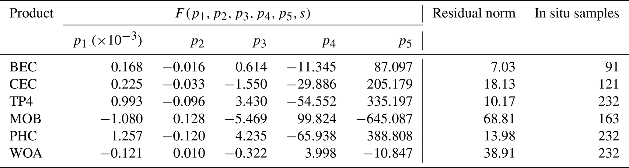
In order to characterize the dependency of the bias on the SSS values for the six SSS products, we used the in situ data, plotting their absolute differences as a function of observed SSS in Fig. 12. In general, all products show considerable deviations as high as 8 to 14 psu. While the absolute misfits of most SSS products increase monotonically with lower salinity, the bias of MOB shows a peak around 20 psu (Fig. 12c). A fourth-order polynomial function,
is then fitted to the absolute bias for each SSS product, where S represents the in situ salinity. The fitting coefficients, p1 to p5, are listed in Table 3 for each product. The norm residuals are displayed on each panel in Fig. 12 and clearly show that the fitting for MOB has the largest uncertainty, while the minimal norm residuals are about 10 and 7 psu2, respectively, for BEC and TP4. This suggests the derived fitting curves for BEC and TP4 have relatively credible skill characterizing the error distribution as a function of the observed SSS. Both curves decrease with increasing salinity above 28 (30) psu for BEC (TP4) and increase slightly afterwards. The absolute bias in TP4 is consistently larger than that in BEC. The fitted curves of PHC and WOA have similar functional forms to TP4 and BEC, but with lower amplitudes.
Table 3Optimal coefficients for the fourth-order polynomial fit of the errors (see Eq. 3) as a function of in situ SSS for each product.
To understand the uncertainties in the Arctic SSS, our study evaluates two gridded SMOS SSS products (BEC and CEC), two CMEMS products (TP4 and MOB), and two climatology products (PHC and WOA) by mutual intercomparison and comparisons with both dependent and independent in situ datasets during the years 2011–2013.
The differences in spatial coverage of the two SMOS SSS were shown in the monthly mean (Figs. 2 and 3), due to the different retrievals applied in these two datasets. The spatial distributions of SSS from TP4 and PHC are close to each other, due to the relaxation of the TOPAZ model towards PHC. Relative to TP4, the SSS deviations of the four products (BEC, MOB, WOA, and PHC) in summer show similar magnitude over open waters. By contrast, the CEC SSS shows a negative bias (< −1 psu) over the region extending from Iceland towards the western side of Ireland (Figs. 4, 5), but the BEC SSS has a slightly but clear negative bias over the region. In general, the most significant differences in the SSS deviations relative to TP4 are found under the sea-ice cover and in its surrounding marginal ice zones.
Furthermore, the intercomparison of the SSS products shows that the BEC SSS in August and September (Figs. 4, 5) has consistent negative deviations along the sea-ice edge in the Beaufort Sea and the Chukchi Sea, but the CEC SSS has opposite deviations in these 2 months. Thus, it seems that the two SMOS products would give rise to significantly different effects on the upper ocean state, were they assimilated.
Focusing on the wider Arctic domain (> 60∘ N), the deviations of the five SSS products relative to TP4 show diverse seasonal characteristics (Fig. 6). Although the BEC and CEC SSS products show similar deviations of 1.5 psu (Fig. 6a) in summer, the BEC deviations in winter are clearly lower (∼0.5 psu). The deviations of MOB and WOA (Fig. 6a) vary from over 1.5 psu in winter to around 4 psu in summer, so all are in considerable disagreement with TP4. Consequently, our intercomparison suggests that the BEC SSS has a pattern more consistent with the TP4 SSS among the SSS products compared here.
The in situ data from CORA5.1, which were used in both TP4 and MOB, have been used for evaluation of the six SSS products in eight sub-regions (Fig. 1a). These were divided into two parts: the central – seasonally ice-covered – Arctic Ocean and the open ocean areas (the northern North Atlantic Ocean and the Nordic Seas). Due to limited coverage of BEC and CEC in S1, the scatterplots (Fig. 7) show a positive saline bias (> 4 psu) for low-salinity water (< 27 psu). However, the salinity bias of BEC is slightly reduced for relatively higher-salinity water (> 27 psu). In the Kara Sea and the Barents Sea, the TP4 SSS has a minimal RMSD compared with others (Table 2). The BEC scatterplots in S2 and S3 (Fig. 7) are similar to TP4.
In the northern North Atlantic Ocean and the Nordic Seas (Fig. 8), the scatterplots of the CEC SSS show that it underestimates the Atlantic water salinity, which is also consistent with the intercomparison results (low-salinity deviation) shown in Figs. 4 and 5. The misfits of the mean and RMSDs shown in Figs. 9 and 10 suggest that the CEC SSS has considerable uncertainty (RMSD of about 1 psu), especially in the Nordic Seas with an obvious low-salinity bias. By comparison, the SSS uncertainties of BEC are significantly lower than CEC and are equivalent to both TP4 and PHC. Two notable regions, where the BEC SSS has lower uncertainties than TP4 against the in situ observations are along the Norwegian coast and near the west coast of Greenland. It is reasonable to expect that they should benefit the most if the BEC SSS were successfully assimilated into the TOPAZ system.
Against independent in situ observations from BGEP and CLIVAR, the SSS evaluation in the Beaufort Sea is performed in three successive summers. The linear regression against these independent SSS observations (Fig. 11) shows that the BEC SSS has the smallest RMSD of 1.8 psu with a positive bias of 0.1 psu, and the CEC SSS has a larger RMSD of about 3.8 psu with a larger positive bias of 2.4 psu (Fig. 11). On the other hand, the TP4 SSS also shows a large RMSD of about 3.6 psu with a large positive bias of 2.6 psu. These are smaller than MOB which has an RMSD of 8.2 psu and a larger negative bias (−5.0 psu). As for the two climatology products, the RMSDs of WOA and PHC are both above 2.8 psu but with a significantly smaller bias in WOA. More specifically, the poor fit of all products is attributed to large product–observation mismatches against in situ salinity observations below 24 psu, which are located over the continental shelf near the estuary of the Mackenzie River.
In order to characterize the product–data misfits of all six products against in situ data, a fourth-order polynomial is fitted to the absolute deviation as a function of the observed salinity (Fig. 12). The absolute deviations of most of the products except MOB decrease monotonically with increasing salinity. The norm residuals for TP4 and BEC are the smallest among all six products with 10.2 and 7.0, respectively. The fitted curve reaches its smallest value of below 1.0 psu for an in situ salinity of 28 and 30 psu for BEC and TP4, respectively. Both the fitted curves for CEC and MOB have large norm residuals of 18.1 and 68.8 psu2, respectively. Note that special attention must be paid when using MOB in the Arctic Ocean due to a large negative bias and high RMSD in regions where the product is based on a limited number of observations.
The above evaluations suggest that certain benefits can be expected in assimilating the BEC SSS into the TOPAZ Arctic ocean analysis–forecast system. The knowledge of the error structure in the SSS products provided in this study will serve as input to the observation error for the SMOS product, as required by data assimilation. The poor spatial coverage of CORA in situ data in the Arctic Ocean urgently requires more data – especially from the Arctic Ocean marginal seas – to be compiled from an independent data source to validate the SMOS SSS products. In addition, when comparing the two climatology products, PHC and WOA, the SSS scatterplots of the PHC in the central Arctic (Fig. 7) reveal a saline bias for low-salinity waters. Considering that PHC does not include the two more recent decades of data (Table 1), this confirms that the freshening in the Canadian Basin since the 1990s is rather significant as discussed by Morison et al. (2012). Based on this, the next TOPAZ system will use WOA in replacement of PHC as target relaxation data.
The SSS products of TP4 and MOB used in this paper are freely available from CMEMS (http://marine.copernicus.eu, last access: August 2019). The two SMOS L3 SSS and the climatology SSS are distributed by the respective websites listed in Table 1. The in situ observation of CORA5.1 is also freely available from the CMEMS port, and other independent in situ profiles from BGEP and CLIVAR are accessible as the states in Sect. 2.3.
JX initiated the collaboration and designed the study. LB and RR contributed the result interpretation. AS enhanced the figure quality. TW collected the in situ data from CLIVAR. JX led the writing phase, with LB, RR, AS, and TW contributing to editing and review. All authors worked on the paper.
The authors declare that they have no conflict of interest.
This article is part of the special issue “The Copernicus Marine Environment Monitoring Service (CMEMS): scientific advances”. It is not associated with a conference.
The authors acknowledge the support of CMEMS for the Arctic MFC and funding from the European Space Agency project Arctic+Salinity. Grants of computing time (nn2993k and nn9481k) and storage (ns2993k) from the Norwegian Sigma2 infrastructures are gratefully acknowledged. The BEC SSS is provided by the Barcelona Expert Centre (http://bec.icm.csic.es/, last access: July 2019), Spain. The CEC SSS is distributed by the Ocean Salinity Expertise Center (CECOS) of CATDS at IFREMER, France. We thank two anonymous reviewers for constructive suggestions that have improved this paper.
This research has been supported by the CMEMS for the Arctic MFC (grant no. 69) and the European Space Agency project Arctic + Salinity (ref. ITT: EOP-SDR/SWO/084-17/DFP).
This paper was edited by Ananda Pascual and reviewed by two anonymous referees.
Bertino, L. and Lisæter, K. A.: The TOPAZ monitoring and prediction system for the Atlantic and Arctic Oceans, J. Oper. Oceanogr., 1, 15–19, https://doi.org/10.1080/1755876X.2008.11020098, 2008.
Boutin, J., Vergely, J. L., Marchand, S., D'Amico, F., Hasson, A., Kolodziejczyk, N., Reul, N., Reverdin, G., and Vialard, J.: New SMOS Sea Surface Salinity with reduced systematic errors and improved variability, Remote Sens. Environ., 214, 115–134, https://doi.org/10.1016/j.rse.2018.05.022, 2018.
Buongiorno Nardelli, B., Droghei, R., and Santoleri, R.: Multi-dimensional interpolation of SMOS sea surface salinity with surface temperature and in situ salinity data, Remote Sens. Environ., 180, 392–402, https://doi.org/10.1016/j.rse.2015.12.052, 2016
Cabanes, C., Grouazel, A., von Schuckmann, K., Hamon, M., Turpin, V., Coatanoan, C., Paris, F., Guinehut, S., Boone, C., Ferry, N., de Boyer Montégut, C., Carval, T., Reverdin, G., Pouliquen, S., and Le Traon, P.-Y.: The CORA dataset: validation and diagnostics of in-situ ocean temperature and salinity measurements, Ocean Sci., 9, 1–18, https://doi.org/10.5194/os-9-1-2013, 2013.
Chassignet, E. P., Smith, L. T., and Halliwell, G. R.: North Atlantic Simulations with the Hybrid Coordinate Ocean Model (HYCOM): Impact of the vertical coordinate choice, reference pressure, and thermobaricity, J. Phys. Oceanogr., 33, 2504–2526, https://doi.org/10.1175/1520-0485(2003)033<2504:NASWTH>2.0.CO;2, 2003.
D'Addezio, J. M. and Subrahmanyam, B.: Sea surface salinity variability in the Agulhas Current region inferred from SMOS and Aquarius, Remote Sens. Environ., 180, 440–452, https://doi.org/10.1016/j.rse.2016.02.006, 2016.
de Boyer Montegut, C., Madec, G., Fischer, A., Lazar, A., and Iudicone, D.: Mixed Layer Depth over the Global Ocean: An Examination of Profile Data and a Profile-Based Climatology, J. Geophys. Res., 109, 1–20, https://doi.org/10.1029/2004JC002378, 2004.
Drange, H. and Simonsen, K.: Formulation of air-sea fluxes in the ESOP2 version of MICOM, Technical Report No. 125 of Nansen Environmental and Remote Sensing Center, 1996.
Droghei, R., Buongiorno Nardelli, B., and Santoleri, R.: A new global sea surface salinity and density dataset from multivariate observations (1993–2016), Front. Mar. Sci, 5, 84, https://doi.org/10.3389/fmars.2018.00084, 2018.
ESA: SMOS data products, available at: https://earth.esa.int/documents/10174/1854456/SMOS-Data-Products-Brochure (last access: 12 December 2018), 2017.
Font, J., Camps, A., Borges, A., Martín-Neira, M., Boutin, J., Reul, N., Kerr, Y. H., Hahne, A., and Mecklenburg, S.: SMOS: The challenging sea surface salinity measurement from space, Proc. IEEE, 98, 649–665, https://doi.org/10.1109/JPROC.2009.2033096, 2010.
Furue, R., Takatama, K., Sasaki, H., Schneider, N., Nonaka, M., and Taguchi, B.: Impacts of sea-surface salinity in an eddy-resolving semi-global OGCM, Ocean Modell., 122, 36–56, https://doi.org/10.1016/j.ocemod.2017.11.004, 2018.
Hátún, H., Sandø, A. B., Drange, H., Hansen, B., and Valdimarsson, H.: Influence of the Atlantic Subpolar Gyre on the Thermohaline Circulation, Science, 309, 1841–1844, https://doi.org/10.1126/science.1114777, 2005.
Hunke, E. C. and Dukowicz, J. K.: An elastic-viscous-plastic model for sea ice dynamics, J. Phys. Oceanogr., 27, 1849–1867, https://doi.org/10.1175/1520-0485(1997)027<1849:AEVPMF>2.0.CO;2, 1997.
Johnson, G. C., Schmidtko, S., and Lyman, J. M.: Relative contributions of temperature and salinity to seasonal mixed layer density changes and horizontal density gradients, J. Geophys. Res., 117, C04015, https://doi.org/10.1029/2011JC007651, 2012.
Kerr, Y. H., Waldteufel, P., Wigneron, J. P., Delwart, S., Cabot, F., Boutin, J., Escorihuela, M. J., Font, J., Reul, N., Gruhier, C., Juglea, S., Drinkwater, M. R., Hahne, A., Martín-Neira, M., and Mecklenburg, S.: The SMOS mission: New tool for monitoring key elements of the global water cycle, Proc. IEEE, 98, 666–687, https://doi.org/10.1109/JPROC.2010.2043032, 2010.
Kolodziejczyk, N., Boutin, J., Vergely, J.-L., Marchand, S., Martin, N., and Reverdin, G.: Mitigation of systematic errors in SMOS sea surface salinity, Remote Sens. Environ., 180, 164–177, https://doi.org/10.1016/j.rse.2016.02.061, 2016.
Latif, M., Roeckner, E., Mikolajewicz, U., and Voss, R.: Tropical stabilization of the thermohaline circulation in a greenhouse warming simulation, J. Climate, 13, 1809–1813, 2000.
Macdonald, R. W., Carmack, E. C., McLaughlin, F. A., Falkner, K. K., and Swift, J. H.: Connections among ice, runoff and atmospheric forcing in the Beaufort Gyre, Geophys. Res. Lett., 26, 2223–2226, 1999.
Maes, C., Ando, K., Delcroix, T., Kessler, W. S., McPhaden, M. J., and Roemmich, D.: Observed correlation of surface salinity, temperature and barrier layer at the eastern edge of the western Pacific warm pool, Geophys. Res. Lett., 33, L06601, https://doi.org/10.1029/2005GL024772, 2006.
Mathis, J. T. and Monacci, N. M.: Carbon Dioxide and Hydrographic data obtained during the USCGC Healy Cruise HLY1203 in the Arctic Ocean (October 05–25, 2012), available at: http://cdiac.ess-dive.lbl.gov/ftp/oceans/CARINA/Healy/HLY-12-03/ (last access: March 2019), Oak Ridge National Laboratory, US Department of Energy, Oak Ridge, Tennessee, https://doi.org/10.3334/CDIAC/OTG.CLIVAR_33HQ20121005, 2014.
McPhee, M. G., Stanton, T. P., Morison, J. H., and Martinson, D. G.: Freshening of the upper ocean in the Arctic: is perennial sea ice disappearing?, Geophys. Res. Lett., 25, 1729–1732, 1998.
Mecklenburg, S., Drusch, M., Kerr, Y. H., Font, J., Martiìn-Neira, M., Delwart, S., Buenadicha, G., Reul, N., Daganzo-Eusebio, E., Oliva, R., and Crapolicchio, R.: ESA's soil moisture and ocean salinity mission: Mission performance and operations, IEEE TGARS, 50, 1354–1366, https://doi.org/10.1109/TGRS.2012.2187666, 2012.
Mignot, J. and Frankignoul, C.: On the interannual variability of surface salinity in the Atlantic, Clim. Dynam., 20, 555–565, https://doi.org/10.1007/s00382-002-0294-0, 2003.
Morison, J., Kwok, R., Peralta-Ferriz, C., Alkire, M., Rigor, I., Andersen, R., and Steele, M.: Changing arctic ocean freshwater pathways, Nature, 481, 66–70, 2012.
Olmedo, E., Gabarró, C., González-Gambau, V., Martínez, J., Ballabrera-Poy, J., Turiel, A., Portabella, M., Fournier, S., and Lee, T.: Seven Years of SMOS Sea Surface Salinity at High Latitudes: Variability in Arctic and Sub-Arctic Regions, Remote Sens., 10, 1772, https://doi.org/10.3390/rs10111772, 2018.
Reverdin, G., Cayan, D., and Kushnir, Y.: Decadal variability of hydrography in the upper northern North Atlantic in 1948–1990, J. Geophys. Res., 102, 8505–8531, https://doi.org/10.1029/96JC03943, 1997.
Sakov, P. and Oke, P. R.: A deterministic formulation of the ensemble Kalman Filter: an alternative to ensemble square root filters, Tellus A, 60, 361–371, https://doi.org/10.1111/j.1600-0870.2007.00299.x, 2008.
Simmons, A., Uppala, S., Dee, D., and Kobayashi, S.: ERA-Interim: New ECMWF reanalysis products from 1989 onwards, ECMWF Newsletter, 110, 25–35, https://doi.org/10.21957/pocnex23c6, 2007.
SMOS Team: SMOS L2 OS Algorithm Theoretical Baseline Document, ESA, Paris, France, SO-TN-ARG-GS-0007, version 3.13, available at: https://earth.esa.int/documents/10174/1854519/SMOS_L2OS-ATBD (last access: 12 December 2018), 2016.
SMOS-BEC Team: Quality Report: Validation of SMOS-BEC experimental sea surface salinity products in the Arctic Ocean and high latitudes Oceans, Years 2011–2013, Barcelona Expert Centre, Spain, Technical note: BEC-SMOS-0007-QR version 1.0, available at: http://bec.icm.csic.es/doc/BEC-SMOS-0007-QR.pdf (last access: 13 December 2018), 2016.
Steele, M. and Ermold, W.: Salinity Trends on the East Siberian Shelves, Geophys. Res. Lett., 31, L24308, https://doi.org/10.1029/2004GL021302, 2004.
Steele, M., Morley, R., and Ermold, W.: PHC: A global ocean hydrography with a high-quality Arctic Ocean, J. Climate, 14, 2079–2087, 2001.
Sumner, D. and Belaineh, G.: Evaporation, Precipitation, and Associated Salinity Changes at a Humid, Subtropical Estuary, Estuaries, 28, 844–855, available at: http://www.jstor.org/stable/3526951 (last access: July 2019), 2005.
Supply, A., Boutin, J., Vergely, J.-L., Martin, N., Hasson, A., Reverdin, G., Mallet, C., and Viltard, N.: Precipitation Estimates from SMOS Sea-Surface Salinity, Q. J. Roy. Meteorol. Soc., 144, 103–119, https://doi.org/10.1002/qj.3110, 2018.
Talley, L. D., Johnson, G. C., Purkey, S., Feely, R. A., and Wanninkhof, R.: Global Ocean Ship-based Hydrographic Investigations Program (GO-SHIP) provides key climate-relevant deep ocean observations, US CLIVAR Variations, 15, available at: https://www.pmel.noaa.gov/pubs/PDF/tall4659/tall4659.pdf (last access: 19 December 2018), 2017.
Toole, J. M., Krishfield, R. A., Timmermans, M.-L., and Proshutinsky, A.: The Ice-Tethered Profiler: Argo of the Arctic, Oceanography, 24, 126–135, https://doi.org/10.5670/oceanog.2011.64, 2011.
Tseng, Y., Bryan, F. O., and Whitney, M. M.: Impacts of the representation of riverine freshwater input in the community earth system model, Ocean Modell., 105, 71–86, https://doi.org/10.1016/j.ocemod.2016.08.002, 2016.
Uotila, P., Goosse, H., Haines, K., Chevallier, M., Barthélemy, A., Bricaud, C., Carton, J., Fučkar, N., Garric, G., Iovino, D., Kauker, F., Korhonen, M., Lien, V. S., Marnela, M., Massonnet, F., Mignac, D., Peterson, A., Sadikn, R., Shi, L., Tietsche, S., Toyoda, T., Xie, J., and Zhang, Z.: An assessment of ten ocean reanalyses in the polar regions, Clim. Dynam., 52, 1613–1650, https://doi.org/10.1007/s00382-018-4242-z, 2019.
Vancoppenolle, M., Fichefet, T., and Goosse, H.: Simulating the mass balance and salinity of Arctic and Antarctic sea ice, 2, Importance of sea ice salinity variations, Ocean Modell., 27, 54–69, https://doi.org/10.1016/j.ocemod.2008.11.003, 2009.
Verbrugge, N., Mulet, S., Guinehut, S., Buongiorno Nardelli, B., and Droghei, R.: Quality information document for global ocean multi observation products multiobs_glo_phy_rep_015_002, CMEMS-MOB-QUID-015-002, v1.0, available at: http://cmems-resources.cls.fr/documents/QUID/CMEMS-MOB-QUID-015-002.pdf (last access: 14 December 2018), 2018.
Vialard, J. and Delecluse, P.: An OGCM study for the TOGA decade: I. Role of salinity in the physics of the Western Pacific fresh pool, J. Phys. Oceanogr., 28, 1071–1088, 1998.
Xie, J., Counillon, F., Bertino, L., Tian-Kunze, X., and Kaleschke, L.: Benefits of assimilating thin sea ice thickness from SMOS into the TOPAZ system, The Cryosphere, 10, 2745–2761, https://doi.org/10.5194/tc-10-2745-2016, 2016.
Xie, J., Bertino, L., Counillon, F., Lisæter, K. A., and Sakov, P.: Quality assessment of the TOPAZ4 reanalysis in the Arctic over the period 1991–2013, Ocean Sci., 13, 123–144, https://doi.org/10.5194/os-13-123-2017, 2017.
Xie, J., Counillon, F., and Bertino, L.: Impact of assimilating a merged sea-ice thickness from CryoSat-2 and SMOS in the Arctic reanalysis, The Cryosphere, 12, 3671–3691, https://doi.org/10.5194/tc-12-3671-2018, 2018.
Yu, L.: A global relationship between the ocean water cycle and near-surface salinity, J. Geophys. Res., 116, C10025, https://doi.org/10.1029/2010JC006937, 2011.
Zweng, M. M., Reagan, J. R., Antonov J. I., Locarnini, R. A., Mishonov, A. V., Boyer, T. P., Garcia, H. E., Baranova, O. K., Johnson, D. R., Seidov, D., and Biddle, M. M.: World Ocean Atlas 2013, Volume 2: Salinity, edited by: Levitus, S. and Mishonov, A., Technical Ed. NOAA Atlas NESDIS 74, 39 pp., 2013.