2.1 Atmosphere component and surface forcing

In the CPLDA system, analysis and forecast fluxes are calculated using bulk formulae based on COARE3.0 (Fairall et al., 2003) within the Unified Model (MetUM) atmosphere at 40 km resolution and interpolated and passed to the NEMO ocean component by the OASIS3 coupler (Valcke, 2006). The FOAM system used interpolated atmospheric fields from the operational Met Office global NWP configuration of the MetUM (at 17 km resolution in 2015) with CORE bulk formulae (Large and Yeager, 2004) to calculate the turbulent fluxes. The CPLDA atmospheric component is the GA6.0 (Walters et al., 2017) atmospheric science configuration (also used by GloSea) for both the analysis and forecast, while the NWP configuration used to force FOAM was GA6.1 (note that this distinction mainly relates to aspects of the land surface treatment and is largely irrelevant from the ocean point of view). The CPLDA atmosphere data assimilation system is described in detail in Lea et al. (2015). It uses an incremental strong constraint 4D-Var system similar to Rawlins et al. (2007). One addition to the system described in Lea et al. (2015) is that the CPLDA atmosphere data assimilation now uses a variational bias correction (VarBC) to continuously update the bias correction applied to observations. VarBC (Lorenc, 2013) was not implemented operationally in the NWP system until March 2016; however, all the CPLDA experiments in this paper use VarBC.

Table 1The FOAM , CPLDA and GloSea ocean configurations.

Download Print Version | Download XLSX

2.2 Ocean component

The ocean configuration is described in detail below, and the CPLDA and FOAM ocean components are summarised in Table 1. Both the CPLDA and FOAM systems use the global ocean configuration GO5 (Megann et al., 2014). GO5 uses version 3.4 of the NEMO modelling system (Madec and the NEMO team, 2008) with the ORCA025 tripolar horizontal grid (which has a $\mathrm{1}/\mathrm{4}{}^{\circ }$ or 28 km horizontal grid spacing at the Equator, reducing to 7 km at high southern latitudes and 10 km in the Arctic Ocean) and is based on the configuration developed by Mercator Ocean. The vertical coordinate system is based on geopotential levels using the DRAKKAR 75-level set, which provides an increased near-surface resolution (including 1 m surface layers to help resolve shallow mixed layers and potentially capture diurnal variability) without compromising resolution at depth. The model bathymetry is DRAKKAR v3.3, which is based on the ETOPO1 dataset (Amante and Eakins, 2009) with additional data in coastal regions from GEBCO (General Bathymetric Chart of the Oceans; IOC, IHO and BODC, 2003). Partial cell thicknesses at the ocean floor allow for a better representation of ocean topography and, in combination with an energy- and enstrophy-conserving momentum advection scheme and a free-slip lateral momentum boundary condition, improve the mesoscale circulation, in particular the simulation of western boundary currents. The tracers are advected using a total-variation-diminishing (TVD) scheme (Zalesak, 1979) and a linear filtered free surface is used to remove high-frequency gravity waves. Tracer diffusion is Laplacian along isopycnals, and horizontal momentum diffusion is performed using a bi-Laplacian operator along geopotential levels. The vertical diffusion implemented in the CPLDA system is the turbulent kinetic energy (TKE) scheme of Gaspar et al. (1990) updated to ensure dynamical consistency in the space–time discretisations (Burchard, 2002). The background diffusivity and viscosity include a double diffusive mixing parameterisation and a parameterisation to attempt to model the mixing effect of Langmuir circulation. In CPLDA, both analysis and the forecast use a Haney retroaction to control sea surface salinities, a 3-D Newtonian damping towards a World Ocean Atlas 2001 climatology (to prevent long term drift of subsurface tracer fields) and a pressure gradient bias correction in the tropics (Bell et al., 2004) to ensure temperature and salinity increments are retained by the model. The Haney flux correction (Haney, 1971) is applied to the sea surface salinity (SSS) based on the difference between the model and climatology; the magnitude of the restoring on SSS is −33.33 mm day⁻¹ psu⁻¹. A summary of the settings for the ocean component in FOAM and CPLDA is shown in Table 1. Most settings are identical except for necessary differences in the surface forcing and a shorter assimilation time window for CPLDA. The ocean data assimilation is described in more detail in Sect. 2.5.

2.3 Sea ice component

The sea ice model (CICE version 4.1; Hunke and Lipscomb, 2010) runs on the same ORCA025 grid as NEMO and with five ice thickness categories. The CICE model determines the spatial and temporal evolution of the ice thickness distribution (ITD) due to advection, thermodynamic growth and melt, and mechanical redistribution and ridging (Thorndike et al., 1975). The CPLDA system documented predates the development work described in West et al. (2016) and Ridley et al. (2018). Therefore, when running coupled to the Unified Model (MetUM) atmosphere, the CPLDA system uses the zero-layer thermodynamic model of Semtner (1976), with a single layer of both ice and snow in CICE. The FOAM system, on the other hand, uses a five-layer thermodynamic model (four ice layers and one snow layer). Ice dynamics are calculated using the elastic–viscous–plastic (EVP) scheme of Hunke and Dukowicz (2002). In CPLDA, for both the analysis and forecast, the ice top and bottom conductive heat fluxes are calculated within the atmosphere model, interpolated by OASIS and then passed to NEMO from which they can be accessed by CICE. In GloSea, the heat fluxes calculated by the atmosphere model were also used, but in the FOAM analysis CICE used its own bulk formulation to specify surface boundary conditions.

In FOAM the freezing temperature is dependent on salinity to provide a more realistic representation of ice melting and freezing mechanisms and to give better consistency when assimilating both sea surface temperature and sea ice concentration. For technical reasons the initial coupled DA system assessed here used a fixed freezing temperature of $-\mathrm{1.8}{}^{\circ }$C, as did the GloSea system. However, salinity dependence was later introduced in CPLDA in September 2018. The GSI6 global sea ice configuration used in the CPLDA system is detailed in Rae et al. (2015).

2.4 Ocean observations

The ocean observations assimilated into the CPLDA system are the same as in FOAM. These are as follows.

• Satellite SSTs are from subsampled level 2 data supplied by the Global High-Resolution Sea Surface Temperature (GHRSST) project comprising Advanced Very High Resolution Radiometer data (NOAA & MetOp), microwave AMSR-2 data and Visible Infrared Imaging Radiometer Suite (VIIRS) data. Note that daytime satellite SST data with a strong diurnal signal wherein the wind speed is less than 6 m s⁻¹ are not used.

• In situ SSTs are from moored buoys, drifting buoys and ships (the in situ observations are considered unbiased and used as a reference for satellite SST bias correction).

• Sea level anomaly (SLA) observations are from the Jason-2, Jason-3, CryoSat-2, SARAL–AltiKa and Sentinel-3a platforms.

• Subsurface temperature and salinity profiles are from Argo profiling floats, underwater gliders, moored buoys, marine mammals and manual profiling methods.

• Sea ice concentration is from Special Sensor Microwave Imager/Sounder (SSMIS) data provided by the EUMETSAT Ocean Sea Ice Satellite Application Facility (OSI-SAF) as a daily gridded product on a 10 km polar stereographic projection.

Model fields are mapped into observation space using the NEMO observation operator to create nearest-time-step model counterparts at the observation location using bilinear interpolation in the horizontal and cubic splines in the vertical directions.

2.5 Ocean data assimilation

The CPLDA system is based on a weakly coupled data assimilation approach. The coupled model is used to provide background information for separate ocean, sea ice, atmosphere and land analyses. The increments generated from these separate analyses are added back into the coupled model (Lea et al., 2015).

For the ocean and sea ice DA both FOAM and CPLDA use NEMOVAR (Mogensen et al., 2012) – an incremental 3D-Var, first guess at appropriate time (FGAT) assimilation scheme designed specifically for use with NEMO and further tuned at the Met Office for the $\mathrm{1}/\mathrm{4}{}^{\circ }$ global model (Waters et al., 2013, 2015). The state vector in NEMOVAR consists of temperature, salinity, surface elevation, sea ice concentration and horizontal velocities. Key features of NEMOVAR are the multivariate relationships, which are specified through a linearised balance operator (Weaver et al., 2006), and the use of an implicit diffusion operator to model background error correlations (Mirouze and Weaver, 2010). As detailed in Waters et al. (2013), the NEMOVAR system includes bias correction schemes for both sea surface temperature (SST) and altimeter data (using the CNES-CLS09 mean dynamic topography (MDT) of Rio et al., 2011, as a reference). The temperature and unbalanced salinity are assimilated using two horizontal correlation length scales (Mirouze et al., 2016) following the method described in Martin et al. (2007). FOAM and CPLDA run one outer loop and 40 iterations of the inner loop minimisation of the cost function. Note that the sea ice DA is run in a separate assimilation step to the ocean DA.

Analysis updates are made to the state variables in the NEMO model, with the exception of sea ice concentration updates, which are made in the CICE model. Updates increasing ice concentration are always made to the thinnest category ice, whilst updates decreasing ice concentration are made to the thinnest ice thickness category available in that grid cell (Blockley et al., 2014). The snow thickness on ice is preserved where there is existing ice but initialised to zero where new ice is added to a previously ice-free grid cell (Blockley et al., 2014).

A few technical changes to the FOAM ocean data assimilation system are needed to fit into the coupled framework. The first technical change made was to match the atmosphere cycling. In the FOAM system, the observation operator and incremental analysis update (IAU) are performed in separate NEMO runs. In CPLDA, this has been altered such that the IAU is followed by observation operator in one combined model run. The second major change from FOAM to CPLDA was to reduce the assimilation time window of the ocean from 24 to 6 h to match the time window of the atmosphere (see Lea et al., 2015). The third change was to reduce the period over which the increment is added to the ocean model in the IAU from 24 to 3 h. This choice is in part to ensure that on the 00Z cycle (with window from 21Z to 03Z) the full increments have been added to the ocean state by 00Z. Hence these ocean restarts can subsequently be used, in exactly the same way as 00Z ocean restarts from FOAM, by groups running initialised coupled forecasts. It is also important to note that differences in observation cutoff due to differences in operational scheduling impact the number of observations assimilated by each system.

No specific tuning has been made for the coupled system. The error covariances used in CPLDA were calculated in the context of the uncoupled FOAM system with a 24 h cycle. It is expected that we would improve the DA results by recalculating the error covariances for a coupled model and for a 6 h window (this is planned for future work).

2.6 Experiments

In order to assess the CPLDA system, we ran a 13-month calibration period from 1 January 2015 to 31 January 2016 with 6 h analysis and daily 7 d forecast. To allow parallel running, the 13 months were realised in two sections, each starting from “uncoupled” initial conditions from the FOAM and NWP operational analyses. The first section was from 1 December 2014 to 30 June 2015, whilst the second section was from 1 June 2015 to 31 January 2016. For both sections, the first month is taken as a spin-up period and discarded. No discontinuity has been observed between June 2015 from the first section and July 2015 from the second section, so all assessments undertaken consider the whole of 2015. Every 6 h, a delayed “best analysis” runs 24 h behind real time with a catch-up to real time only required to launch the 7 d forecasts on the 00Z cycle. For running delayed time trials, like that for 2015 described in this paper, the operational availability of observations is replicated by using receipt time information when they are extracted from the Met Office observations database (MetDB). In the following sections, we assess the CPLDA system against the ocean-only FOAM system for the 2015 period. FOAM has been used as the Met Office operational ocean forecasting system for many years. It uses atmospheric forcing from the Met Office NWP operational system and is described in detail in Blockley et al. (2014). Differences between the CPLDA and FOAM ocean configurations are shown in Table 1. There are a few differences between the CPLDA system assessed in the majority of this paper and the final operational implementation. As the systems were running for different periods, observations not available or not yet operationally implemented in 2015 (Jason-3 and Sentinel-3 sea level anomaly data and VIIRS sea surface temperatures) are only assimilated in the final operational version. More significantly, the scheduling of the operational system has been modified to allow additional observations to be assimilated. The result of these changes is that the best analysis runs further behind real time on the 06Z, 12Z and 18Z cycles (42, 36 and 30 h, respectively, compared to 24 h previously). As for the 2015 trial the catch-up to real time is only required to launch the forecast (operationally this is now 10 d) once per day on the 00Z cycle. Where any results are shown from the CPLDA system running with this modified scheduling (as opposed to that used in the 2015 trial), this is clearly indicated.

Additional experiments have been undertaken using the ocean-only FOAM system to look at the impact of running the data assimilation with a shorter assimilation window. The FOAM system was run in hindcast mode (forecasts were not generated) for 6 months from 1 March to 31 August 2018 with the analysis length and assimilation window set to 6 and 24 h. These experiments should decompose the effect of the shortened assimilation window from the effect of the coupling and aid in the interpretation of the comparisons to the FOAM system described herein.

3.1 Sea surface height

CPLDA 2015 and FOAM sea surface height are assessed against observations using class 4 statistics (Ryan et al., 2015). The observations used are provided by CMEMS and include data from the AltiKa, CryoSat-2 and Jason-2 satellites. Altimeter bias correction is applied to the observations. For each model comparison against the satellite observations, the model's own altimeter bias is used. This is important because the altimeter bias contains information from the model mesoscale, so correcting observations using the altimeter bias from one model to assess a second model penalises this second model. Figure 1 shows a time series of the sea level anomaly (SLA) difference statistics assessed against CMEMS observations. In the 2015 experiment with the original scheduling, the CPLDA SLA root mean square error (RMSE) is significantly larger than the FOAM SLA RMSE (Fig. 1a). The larger RMSE in CPLDA can be attributed to the difference in the number of SLA observations assimilated. Figure 2 shows the number of observations assimilated daily by both systems in 2015; the number assimilated by CPLDA is significantly smaller than the number assimilated by FOAM. Differences in scheduling can explain this; the CPLDA 2015 experiment best analysis runs earlier in the day than the comparable FOAM analysis, so fewer observations are available. Following these results, the scheduling of the CPLDA operational system was updated in April 2018. The best analyses at 06Z, 12Z and 18Z are now delayed allowing more observations to be assimilated, as already described in Sect. 2. This change, along with a change in the Met Office database (MetDB), allowing a more frequent ingestion of SLA observations, has resulted in a significant reduction of the CPLDA RMSE (see Fig. 1b). The experiments using the FOAM system to look at the effect of the shorter assimilation window in CPLDA showed no significant difference in SLA statistics between the 6 and 24 h systems.

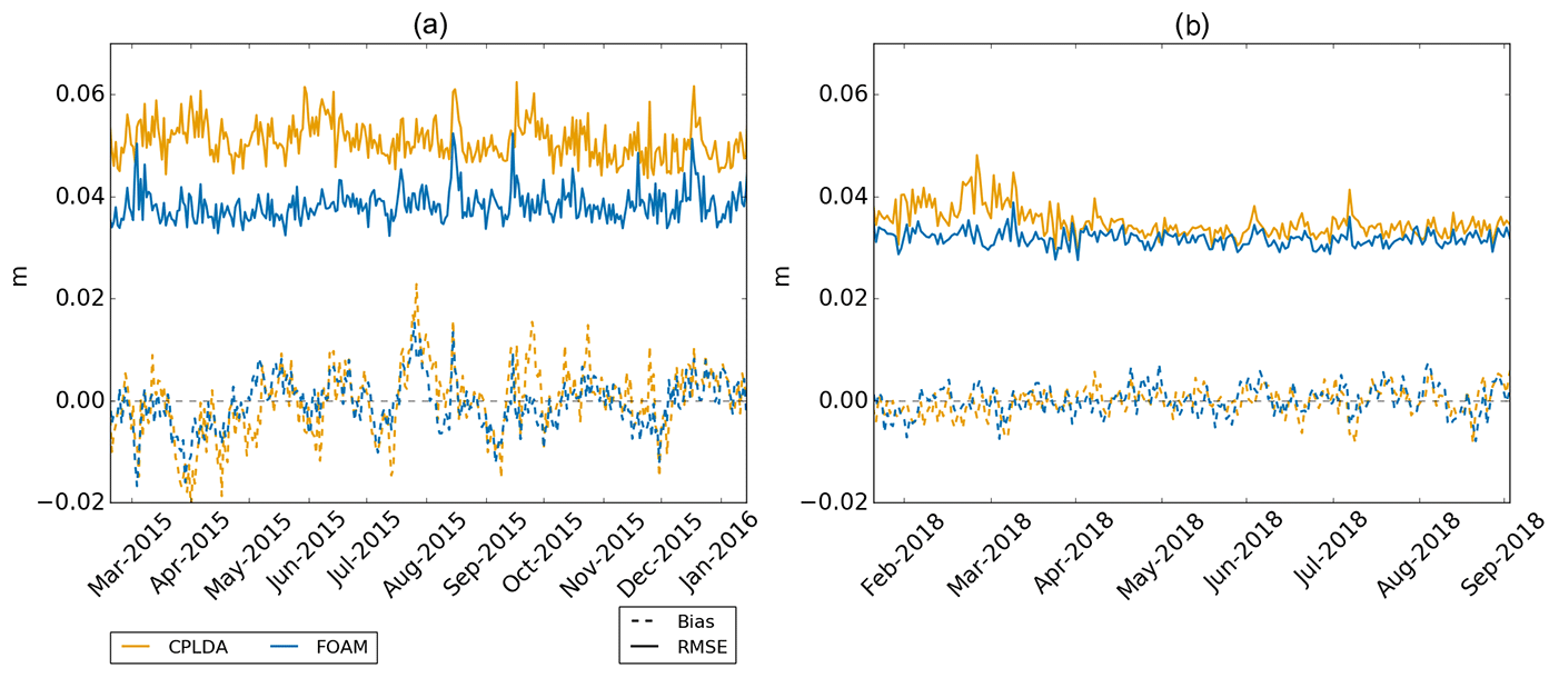
Figure 1SLA class 4 statistics with respect to the CMEMS satellite product (Jason2, CryoSat-2 and AltiKa) for CPLDA and FOAM. (a) For the long CPLDA experiment in 2015 with the old scheduling. (b) From the operational systems for 2018; the CPLDA scheduling was updated to allow more observations to be assimilated in April 2018.

Download

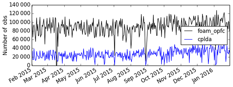
Figure 2Daily number of SLA observations assimilated in the FOAM operational system for 2015 (black line, foam_opfc) and in the CPLDA 2015 experiment (blue line, cplda).

Download

3.2 Sea ice

Figure 3 shows the sea ice extent and volume, respectively, for CPLDA and FOAM best analyses. It shows that the sea ice extent is similar between CPLDA and FOAM and is also comparable to OSTIA. Figure 3 shows that the sea ice volumes are similar in the Arctic, but in the Antarctic CPLDA has a reduced volume compared to FOAM in the Southern Hemisphere winter and spring. Differences in volume can be attributed to differences in sea ice thickness probably caused by differences in freezing temperature treatment. Figure 4 shows the sea ice extent forecast for the melting season in the Arctic (August) and Antarctic (February) for CPLDA and FOAM. Both models have the tendency to melt too much ice during the forecast, especially in the Arctic; in the Antarctic the exaggerated melting in CPLDA is slightly reduced compared to that observed in FOAM. The differences in freezing temperature treatment referred to in Sect. 2.3 may have impacted the sea ice simulation.

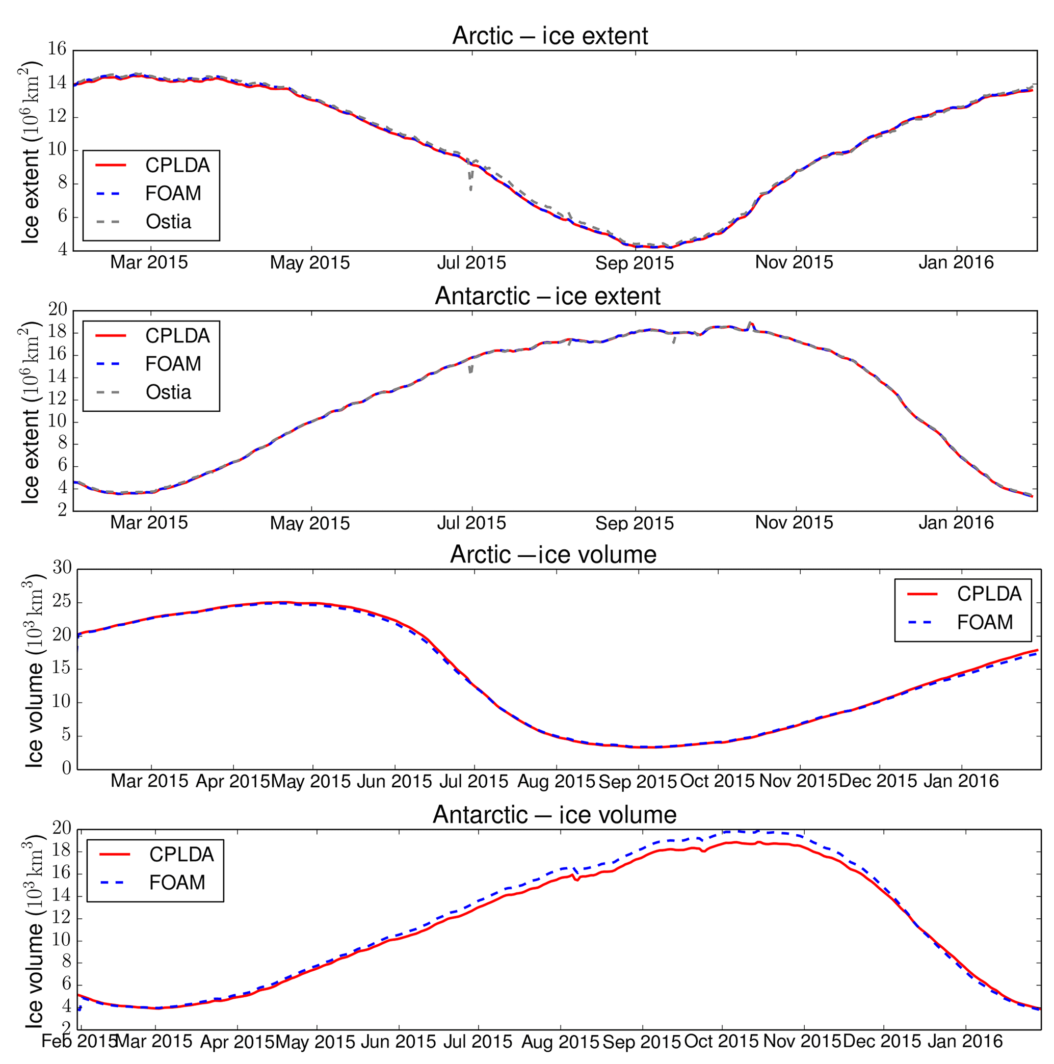
Figure 3Time series of sea ice extent and sea ice volume for CPLDA (2015 experiment) and FOAM.

Download

Figure 4Sea ice extent forecast for CPLDA (2015 experiment) and FOAM during the melting season (February in the Antarctic and August in the Arctic).

Download

3.3 Sea surface temperature

We present class 4 statistics against in situ drifting buoy observations provided by US GODAE. The model SST is defined to be the temperature of the top ocean model grid box, which is at a depth of 0.5 m. The RMSE and mean bias statistics for the CPLDA analysis and forecast are shown in Fig. 5 and compared to FOAM, PSY4 and GloSea statistics. A small cold bias (−0.02 K) is present in CPLDA in the analysis but does not increase during the forecast. In comparison, the coupled forecast from the GloSea system initialised from the uncoupled system exhibits a warm bias significantly increasing during the forecast (+0.09 K after 132 h; Fig. 5a). CPLDA is the only system showing a cold bias; the two uncoupled systems FOAM and PSY4 have a small warm bias. Experiments investigating reducing the assimilation window from 24 to 6 h in the FOAM system show that the difference observed in bias is unlikely to be due to the shorter assimilation window. The cold bias is therefore more likely related to the differences in heat fluxes between the systems described in Sect. 3.5.

The SST RMSE is reduced in the CPLDA analyses compared to the FOAM analyses (this is also observed for the 12 h forecast). Between the 12 and 36 h forecasts the rate of increase of RMSE is greater in CPLDA than in FOAM so that at a forecast length of 36 h and beyond the RMSE is similar in both systems (Fig. 5a). The shorter data assimilation window in CPLDA (6 h) compared to FOAM (24 h) explains the improved SST analysis RMSE in CPLDA. Experiments investigating reducing the assimilation window in the FOAM system improved SST analysis statistics (both RMSE and bias). This supports the results of Lea et al. (2015), who suggested that with a shorter cycle the SST model errors have less time to grow. The increase in RMSE between the 12 and 36 h forecasts in CPLDA could be due to the analysis overfitting the observations. The analysis fitting the observations too closely improves the statistics for the analysis, but as a consequence there is a quicker degradation during the forecast. Future work is required to assess the magnitude of this overfitting by withholding a subset of observations from the data assimilation (these observations can then be used as an independent validation dataset). The RMSE for analysis SSTs in PSY4 is significantly larger than CPLDA, but unlike CPLDA and FOAM, PSY4 does not assimilate SSTs from drifting buoys directly; instead it assimilates the near-real-time Operational Sea surface Temperature and sea Ice Analysis (OSTIA) (Donlon et al., 2012), in which the drifting buoys have been assimilated. Furthermore, when using grid point verification PSY4 statistics may suffer from a “double penalty” whereby higher-resolution models are often penalised compared to coarser-resolution models for missed or misplaced events or false alarms.

The SST RMSE from all models exhibits a seasonal cycle (Fig. 5b) with an increased RMSE during the Northern Hemisphere summer. This increase can be attributed to the Northern Hemisphere bias of the observing network in terms of the number of observations. During the Northern Hemisphere summer the mixed layer depth is shallow, which leads to a more responsive mixed layer; thus, SST variability is increased, which is reflected in the increase in the global RMSE during these months.

The CPLDA SST analysis is also assessed via comparison with OSTIA (Fig. 6a). The global average CPLDA SST is warmer than OSTIA, with the difference being 0.06 K. This difference corresponds to a known cold bias in the OSTIA analysis relative to independent top-level Argo observations (Roberts-Jones et al., 2012), so it could illustrate a potential bias in OSTIA. However, CPLDA SSTs (from the top 1 m thick model layer) are also expected to differ from OSTIA because they will capture some of the diurnal cycle, while OSTIA is a foundation SST free of diurnal warming. Figure 6b shows the difference between CPLDA and FOAM SST analysis annual means. CPLDA SST is generally colder than FOAM, which corresponds to the biases observed in Fig. 5. The differences between the two systems are much smaller than that observed between OSTIA and CPLDA as expected due to similarity in the ocean models and data. Bimodal differences are observed in the areas with a high SST gradient, such as the western boundary currents, Antarctic Circumpolar Current and in the Zapiola Rise region. These differences are due to differences in the position of SST fronts rather than due to the ability of the two analyses to resolve mesoscale features. To investigate mesoscale feature resolution we calculated the SST spectral power using the method described in Fiedler (2018). The SST spatial variability for each of the experiments was determined by wavenumber auto-spectra analysis. All spectra results were calculated on the native grid of the analysis (ORCA025). For each region of interest, the spectra were calculated along the horizontal coordinates closest to a given latitude. The power spectral density of each latitude was calculated using the Welch's average periodogram method, with 28 degrees of freedom and a Hanning window. The overlapping length for each band averaging was half the band length (Fiedler, 2018). The results for CPLDA and FOAM are very similar; in both systems the effective SST resolution is around 50 km.

On average, the CPLDA temperature increment at the surface is negative (Fig. 6c), meaning that the data assimilation is cooling the model at the surface; this is also an issue in FOAM to a lesser degree and may be due to the underestimation of the wind stress described in Sect. 3.5. The largest increments (both positive and negative) are observed in regions of enhanced SST variability such as the Gulf Stream, Kuroshio current and the Antarctic Circumpolar Current. Large negative increments are also applied in the tropics in regions of tropical instability waves. In the tropical Pacific, the imprint from the Tropical Atmosphere Ocean (TAO) mooring array is clearly visible. Figure 6d shows the difference in temperature increment at the surface between CPLDA and FOAM. Bimodal differences are observed in the regions of enhanced SST variability and at the location of the TAO moorings. The degree to which the increments (and therefore the data assimilation) are responsible for the differences in SST between the two systems shown in Figs. 5 and 6b varies regionally, but large-scale similarities are seen in the pattern of the differences.

Figure 5SST (model minus observation) class 4 statistics with respect to drifting buoys: (a) RMSE and mean biases at various lead times; (b) time series of RMSE and mean biases in the “best analysis” from each system.

Download

Figure 6CPLDA SSTs in 2015 compared to (a) OSTIA (0.06 K) and (b) FOAM (−0.03 K); (c) mean SST increments in 2015 for CPLDA (−0.04 K); (d) mean SST increments in 2015 for CPLDA compared to FOAM (−0.01 K). Values in parentheses are averages for the global ocean.

3.4 Temperature and mixed layer depth

The temperature of CPLDA is assessed against Argo profile observations provided by CMEMS (Wehde et al., 2016). The class 4 global temperature statistics for the best analysis are presented in Fig. 7a. The results for the forecast (not shown) are similar to the best analysis, with the mean bias staying unchanged and the RMSE slightly increasing from 0.67 K at 12 h to 0.73 K at 108 h. CPLDA has a cold bias in the subsurface which is maximum (around 0.1 K) at 10 m and present in the thermocline down to approximately 50 m. A smaller warm bias is present at around 100 m, but this is over a greater depth range so it represents a large amount of heat. A subsurface cold bias is present in the ocean-only FOAM system but with a smaller amplitude. For the CPLDA results shown, the number of profile observations being assimilated was smaller than in FOAM due to differences in the scheduling of assimilation cycles. Even in tests with the operational scheduling (referred to in Sect. 2.6) the subsurface bias in CPLDA persists despite the increased number of observations being assimilated. In both CPLDA and FOAM the temperature RMSE is largest in the thermocline, which highlights its variability; the RMSE is larger in CPLDA than in FOAM.

The temperature profile can be affected by the vertical propagation of surface temperature increments through the water column. King et al. (2018) show that the succession of positive and negative temperature increments has an asymmetric effect on the vertical temperature structure due to the way the temperature increment at the surface is propagated to the bottom of the mixed layer. A negative surface increment weakens the stratification and so deepens the mixed layer; this means that a subsequent positive surface increment is projected deeper. Experiments looking at the assimilation time window in an ocean-only system show that the shorter assimilation cycle in CPLDA (6 h) relative to FOAM (24 h) leads to increased temporal noise in the increments and a deepening of the mixed layer.

In CPLDA the large negative increment applied at the surface (Fig. 7b) is propagated down to approximately 50 m; below this a small warm increment is applied down to approximately 150 m. The fact that the negative increment is projected deeper in CPLDA than in FOAM and the dipolar structure in the vertical is consistent with idealised experiments into the vertical propagation of temperature increments (Robert R. King, personal communication, 2018). CPLDA has a larger negative increment at the surface than FOAM. Below approximately 200 m the magnitude of the average temperature increment is small (Fig. 7b) and the increments applied by CPLDA and FOAM are similar. The differences observed in global average temperature increments are reproduced in the ocean-only assimilation time-window experiments comparing a 6 h to a 24 h window. It is therefore likely that the differences observed in the global temperature increment are due to the shorter assimilation window in CPLDA.

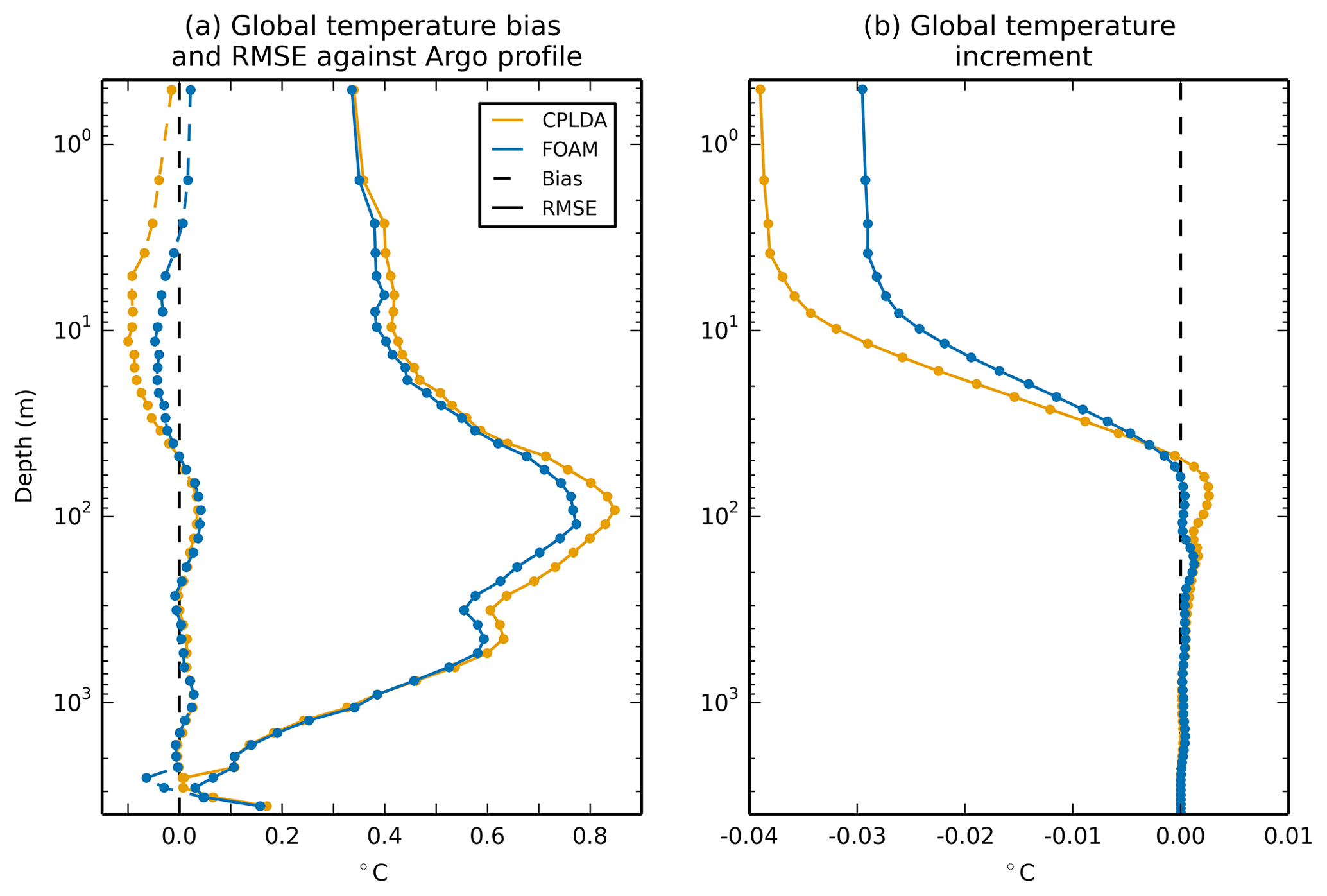
Figure 7(a) CPLDA and FOAM global average mean bias and RMSE temperatures compared to Argo observations using class 4 methodology; (b) global average mean temperature increments applied in CPLDA and FOAM.

Download

Mixed layer depth statistics from the analysis confirm that CPLDA has a deeper MLD than the assimilated profile observations. The MLD statistics presented here use the Kara mixed layer depth with density-based criteria. CPLDA mean error against the assimilated observations is 5.2 m too deep, while the RMSE is 34.7 m. Similarly, the MLD in FOAM is deeper than the observations but both the mean error (2.1 m too deep) and the RMSE (32.6 m) are reduced. These statistics confirm that the CPLDA MLD is deeper than FOAM (Fig. 8). During the forecast MLD RMSE and bias persist for both systems (not shown). Experiments running FOAM with a 6 h assimilation time window show that the shorter window results in an over-deepening of the MLD by 2.9 m relative to that using a 24 h window; this is consistent with the 3.1 m difference observed between CPLDA and FOAM. The change in MLD due to the shorter assimilation window may be caused by the asymmetric effect of the surface temperature increment on vertical temperature structure. The over-deepening of the mixed layer will lead to a misplacement of the thermocline, which will contribute to the larger RMSE in the thermocline in CPLDA than in FOAM observed in Fig. 7a. It is worth noting that differences in wind stress between CPLDA and FOAM will also affect the MLD.

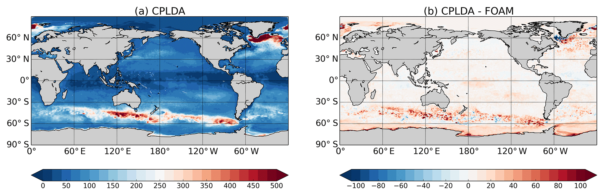
Figure 8Annual mean Kara mixed layer depth in metres (Kara et al., 2000, using a temperature criterion of 0.8 ^∘C): (a) CPLDA and (b) the difference between CPLDA and FOAM. Positive value means CPLDA MLD is deeper than FOAM MLD.

Experiments support the shorter assimilation window in CPLDA causing the differences observed in the global increments (Fig. 7b) and in MLD (Fig. 8) between CPLDA and FOAM. However, these experiments were not able to reproduce the subsurface bias observed in CPLDA relative to FOAM (Fig. 7a). We are currently unable to attribute this bias to the shorter assimilation window. This may be due to the experiments not being long enough (6 months) or more likely that the bias is a result of the differences in forcing between CPLDA and FOAM described in the next section. Future work is planned to look in depth at the vertical propagation of surface increments using a 1-D model and may aid in the attribution of the observed subsurface bias.

3.5 Atmosphere and surface fluxes

In this section, we assess the atmosphere component of CPLDA, focussing on the interface with the ocean, in particular the surface fluxes. We compare CPLDA surface fluxes to FOAM over the ocean; we have not yet investigated the fluxes over the ice. The differences in net total heat flux are shown in Fig. 9. On average, CPLDA receives less heat than FOAM (−3.9 W m⁻²). CPLDA receives less (or loses more) heat in the tropics than FOAM except in the Gulf of Guinea and in the East Pacific along the Peruvian and Chilean coast. At higher latitude, CPLDA loses less heat than FOAM, especially in the regions of large latent heat loss (Kuroshio and Gulf Stream). The reduced heat gain compared to FOAM between 30^∘ S and 30^∘ N contributes to the colder SST observed in CPLDA. The differences in net heat flux compared to FOAM are mainly due to differences in shortwave radiation and particularly in latent heat (Fig. 9). The small-scale pattern differences are due to differences in the representation of the mesoscale between the two models (eddies are not completely constrained by the observations and so are not located in exactly the same positions).

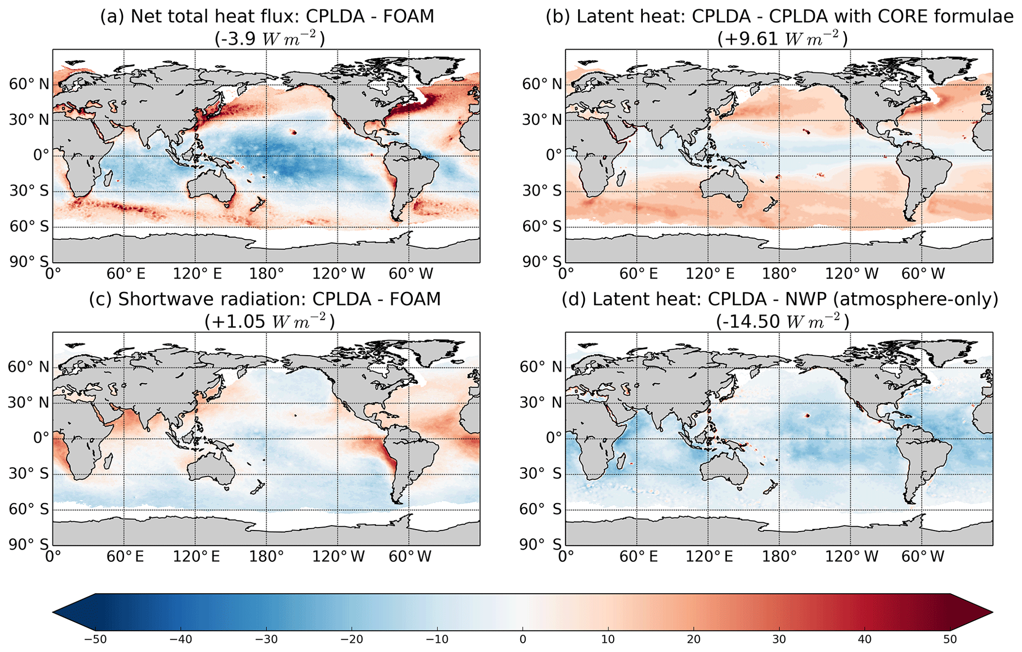
Figure 9Annual mean net downward heat flux differences (W m⁻²): (a) total heat flux difference between CPLDA and FOAM (−3.9 W m⁻²), (b) latent heat flux difference caused by using COARE3.0 bulk formulae in CPLDA rather than CORE as in FOAM (+9.61 W m⁻²), (c) shortwave radiation difference between CPLDA and FOAM (+1.05 W m⁻²), and (d) latent heat difference between CPLDA and the atmosphere-only NWP system, both of which are using COARE3.0 bulk formulae (−14.5 W m⁻²). In brackets are the average values for the global ocean.

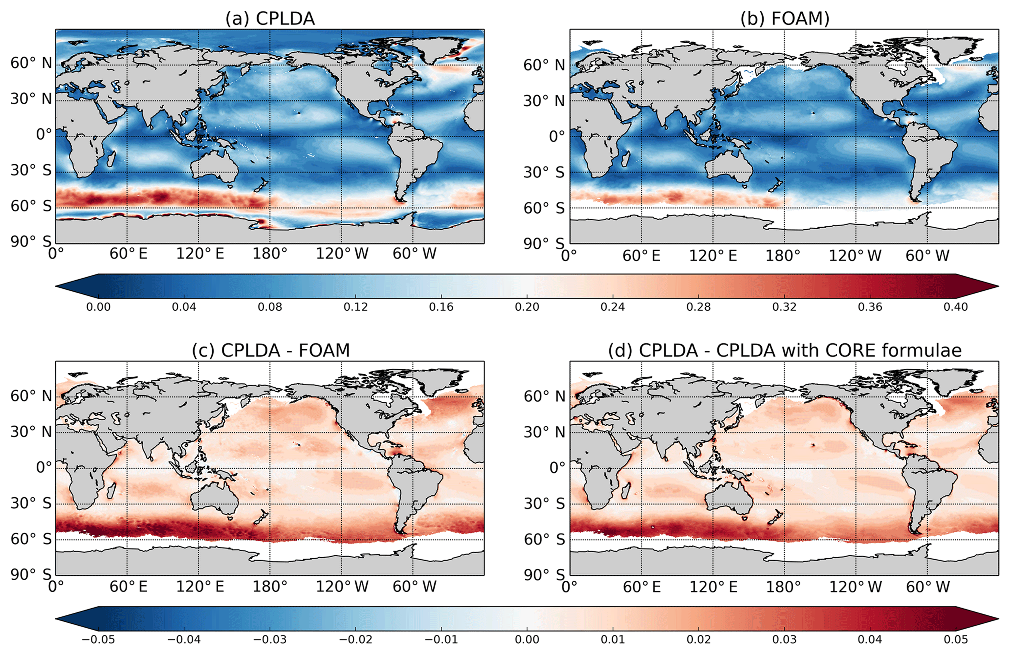
Figure 10Annual mean wind stress magnitude (N m⁻²): (a) CPLDA, (b) FOAM, (c) wind stress difference between CPLDA and FOAM, and (d) wind stress difference caused by using COARE3.0 bulk formulae in CPLDA rather than CORE as in FOAM.

Figure 9c shows the difference in shortwave radiation between CPLDA and FOAM. On average, CPLDA receives more shortwave radiation than FOAM (+1.05 W m⁻²). The difference is large in the Southern Hemisphere where CPLDA receives significantly less shortwave radiation than FOAM. In the equatorial region, CPLDA receives less shortwave radiation in the West Pacific but receives significantly more shortwave radiation than FOAM in the East Pacific and in the Atlantic, including the whole Gulf of Guinea. The stratocumulus clouds are underestimated in the Met Office atmospheric model and cause a shortwave overestimation on the eastern boundary upwelling systems. The differences in shortwave radiation between CPLDA and FOAM in these regions suggest that this bias is larger in CPLDA. In the Northern Hemisphere, CPLDA receives less shortwave radiation in the Pacific, while in the Atlantic it receives more. Overall, the differences observed in shortwave radiation are significant and contribute to the differences observed in total heat fluxes. We have performed a shorter simulation of the CPLDA system with a higher atmospheric resolution (17 km) which gives similar results (not shown) to CPLDA, meaning that the differences in the fluxes between CPLDA and FOAM are not caused by the differences in resolution.

The differences in latent heat can be decomposed into two components. First, the atmosphere component in CPLDA differs from the atmosphere model (NWP) used to force FOAM. Figure 9d shows the difference between CPLDA and NWP latent heat. The NWP latent heat is calculated using the same bulk formulae as CPLDA but is using OSTIA SSTs as a surface boundary condition. This shows that even with the same bulk formulae the evaporation is significantly higher in CPLDA than in NWP. In CPLDA, the air at 10 m is drier than in NWP, causing increased evaporation and increased latent heat loss. The signal is stronger in the tropics and contributes to the differences in total heat flux seen between CPLDA and FOAM, with FOAM losing less heat than CPLDA in the tropics.

Secondly, there are differences in latent heat due to the use of different bulk formulae in CPLDA and FOAM. To investigate the difference caused by the bulk formulae, we recalculated CPLDA fluxes using CORE bulk formulae (Large and Yeager, 2004) as used in FOAM. Figure 9b shows the differences in latent heat when using CORE formulae. At high latitude the latent heat loss is increased, with the largest differences observed in the regions with large latent heat loss. On the other hand, in the equatorial band, the latent heat loss is reduced with CORE formulae. The impact of the bulk formulae on the latent heat calculation is significant and contributes to the differences in total heat flux. An impact is also observed on the sensible heat but with a much smaller magnitude (not shown). The addition of the differences in latent heat caused by having a different atmospheric state (−14.5 W m⁻² Fig. 9d) and those caused by using different bulk formulae (+9.61 W m⁻² Fig. 9b) can explain much of the difference seen in the net heat flux into the ocean between CPLDA and FOAM (Fig. 9a).

The sum of the latent heat differences and shortwave differences equals −3.84 W m⁻² , close to the difference in net total heat flux (−3.9 W m⁻²).

Air–sea momentum flux is a crucial forcing for the ocean as it is through the wind stress that the atmosphere drives the ocean. The CPLDA wind stress magnitude annual mean is shown in Fig. 10a. The wind stress in CPLDA is stronger than in FOAM almost everywhere. The differences in wind stress between CPLDA and FOAM are mainly caused by the different bulk formulae. Indeed, when recalculating CPLDA wind stress using the same (CORE) bulk formulae as FOAM, the differences between CPLDA and the new calculated wind stress are similar to the differences between CPLDA and FOAM (Fig. 10c and d). The new wind stresses are calculated with CORE bulk formulae but using CPLDA wind speed and surface currents. This highlights the importance in the choice of bulk formulae for the wind stress calculation. However, we note that it is not equivalent to running CPLDA using CORE bulk formulae, as reduced wind stress would imply feedback to the atmosphere causing an increase in wind speed and therefore limiting the reduction in wind stress.

Because of the large differences caused by the bulk formulae, comparing the differences in wind stress is equivalent to comparing the different drag coefficient used. Brodeau et al. (2017) highlighted disagreement in the drag coefficient between different bulk formulae, with the COARE 3.0 algorithm producing higher wind stress. They mention that the latest improvements in the COARE algorithm (version 3.5) suggest that the drag coefficient of COARE3.0 is likely too small in strong wind conditions. This suggests that the wind stresses calculated in CPLDA may be underestimated at times, although it is improved compared to those used by FOAM.

3.6 Velocities

Predictions of ocean currents are important for marine activities. They are used for a number of practical applications such as ship routing, marine search and rescue, pollution monitoring, the offshore oil and gas industry, and marine renewable energy. To assess the velocities at 15 m, we compare CPLDA to measurements from drifters. The observations are independent as no ocean current observations are assimilated by the system. We use an in situ delayed-mode product from CMEMS (Etienne, 2017); this is designed for reanalysis purposes with the best available version of in situ data for ocean surface currents. The data are collected from the Surface Drifter Data Assembly Centre (SD-DAC at NOAA AOML). All surface drifter data are processed to check for drogue loss, and a wind slippage correction is applied to undrogued buoys. The wind slip correction is computed following Rio (2012). We compared 15 m model velocities against 15 m CMEMS observations corrected with wind slippage for the year 2015. Despite a limited number of observations compared to SST observations, the observation coverage from drifters is generally good except in the tropical Atlantic.

The class 4 statistics for the 15 m velocities for the global ocean are presented in Fig. 11. On average the CPLDA analysis has a negative bias (−0.07 m s⁻¹) and an RMSE of 0.19 m s⁻¹. In all regions except the tropical Pacific, both the bias and the RMSE are stable during the forecast (not shown). The bias in the uncoupled system analyses (FOAM and PSY4) is the same as CPLDA and the RMSE is close (0.18 for FOAM; 0.17 for PSY4). The larger RMSE in the CPLDA analysis is mainly due to periods of large RMSE in April and November 2015 in the tropical Pacific (see Fig. 11). In regions other than the tropical Pacific no significant differences are observed, with CPDLA and FOAM statistics similar. The increased RMSE in the analysis is caused by spurious currents in the western tropical Pacific (Fig. 12). During the forecast, the currents weaken and the RMSE decreases, suggesting they are caused by the data assimilation. The shorter data assimilation window in CPLDA limits the number of observations and causes noisier increments; in addition, a reduced total number of SLA observations is assimilated in CPLDA compared to FOAM. We re-ran the CPLDA system for a month from 15 October 2015 with the updated scheduling, allowing more observations to be assimilated. In this experiment, the RMSE in the analysis is significantly reduced and now similar to FOAM and PSY4 (see shaded area in Fig. 11). The spurious currents north of Indonesia are suppressed (Fig. 12). However, in the current CPLDA operational system (running with the updated scheduling, allowing more observations to be assimilated), there are still periods with unrealistic currents developing in the western tropical Pacific (not shown). These unrealistic currents caused by SLA assimilation are not present in the FOAM system, which uses the same assimilation scheme and assimilates the same observations as CPLDA. This strongly suggests that they are caused by the shorter assimilation window in CPLDA.

Tuning the error covariances for the shorter time window may reduce or eliminate the above problem. Smaller estimated background errors would give the observation less weight in the analysis and lead to smaller, less noisy increments. Future work investigating re-estimating the background error covariances is planned. The updated CNES-CLS13 mean dynamic topography of Rio et al. (2014) is significantly improved, particularly around the Maritime Continent, compared to the CNES-CLS09 version used in these experiments. Hence, using a newer MDT in the CPLDA system may also reduce this issue.

Figure 11The 15 m velocity using class 4 statistics with respect to velocities derived from drifting buoys for 2015. RMSE and mean bias are shown for CPLDA and FOAM, as well as PSY4 and, for a short test period, CPLDA using the operational scheduling, allowing for the assimilation of additional SLA observations.

Download

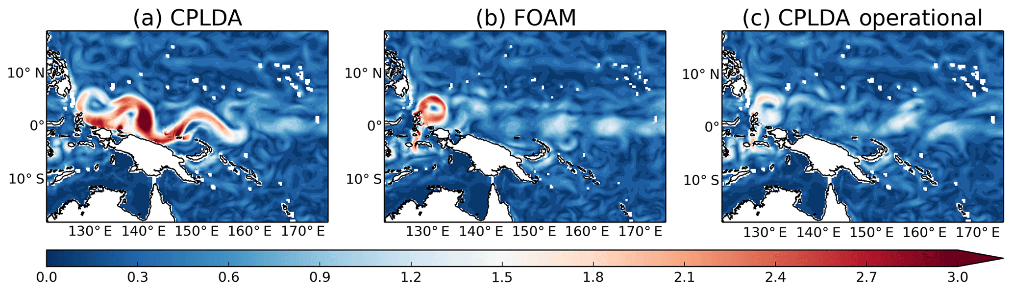
Figure 1215 m velocity average (m s⁻¹) in the western tropical Pacific for the week from 5 to 11 November 2015 for (a) CPLDA, (b) FOAM and (c) CPLDA with the current operational scheduling, allowing for the assimilation of additional SLA observations.

Table 2Velocity class 4 statistics against drifting buoys for 2015 (m s⁻¹).

Download Print Version | Download XLSX

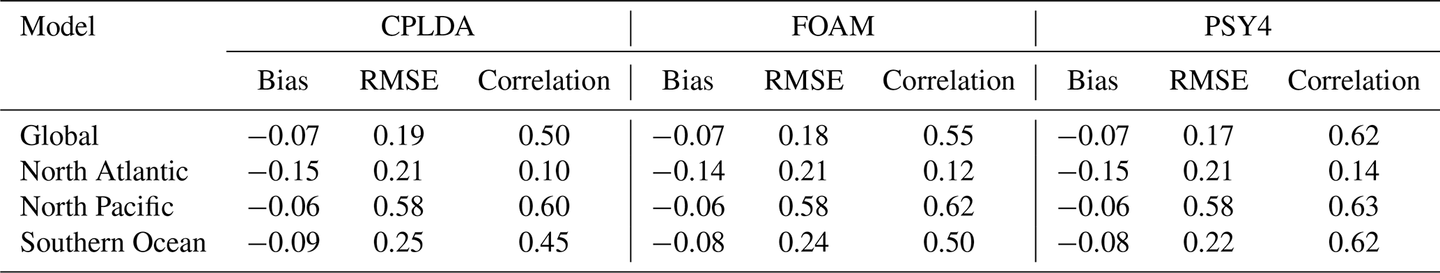
Despite the mean bias and RMSE values, CPLDA velocities are only moderately correlated with observations (0.50). This correlation is weaker than in FOAM (0.55) and PSY4 (0.62). Only PSY4 is skilful using the definition that a correlation greater than 0.6 is an indication of a skilful forecast (Murphy and Epstein, 1989; Hollingsworth et al., 1980). Correlation varies substantially from region to region (Table 2). In some regions, CPLDA correlation is near or above 0.6, as in the North Pacific, while in the North Atlantic the correlation is poor (0.10). All the models have skilful correlation in the North Pacific but poor correlation in the North Atlantic. This was previously observed by Blockley et al. (2012) in an earlier version of the FOAM system. They explained the lack of skill in the North Atlantic by the domination of the mesoscale, which is more difficult to predict, while in more benign regions the model performed better. It is in the Southern Ocean, a region largely dominated by the mesoscale, that the $\mathrm{1}/\mathrm{12}{}^{\circ }$ model (PSY4) most clearly outperforms the $\mathrm{1}/\mathrm{4}{}^{\circ }$ models (CPLDA, FOAM). Here PSY4 has a correlation of 0.62, while CPLDA and FOAM have correlations of 0.45 and 0.50, respectively.

Eddy kinetic energy (EKE) was also compared in CPLDA, FOAM and PSY4. In an ocean-only model, using the ocean velocity to calculate the wind stress has a damping effect on the eddies (Duhaut and Straub, 2006; Dawe and Thompson, 2006; Renault et al., 2016). Despite the expected reduced damping effect in a coupled system, we did not observe a higher EKE in CPLDA than in FOAM. However, at $\mathrm{1}/\mathrm{4}{}^{\circ }$ resolution, the mesoscale is poorly represented and most of the EKE is injected into the model by the SLA assimilation. Hence differences in EKE between CPLDA and FOAM are mainly caused by differences in SLA observations assimilated, or impacts of the shorter assimilation window, rather than due to a reduced eddy damping by the wind stress.