the Creative Commons Attribution 4.0 License.
the Creative Commons Attribution 4.0 License.
 | 08 Nov 2019
Testing the validity of regional detail in global analyses of sea surface temperature – the case of Chinese coastal waters
Yan Li
Hans von Storch
Qingyuan Wang
Qingliang Zhou
Shengquan Tang
We have designed a method for testing the quality of multidecadal analyses of sea surface temperature (SST) in regional seas by using a set of high-quality local SST observations. In recognizing that local data may reflect local effects, we focus on the dominant empirical orthogonal functions (EOFs) of the local data and of the localized data of the gridded SST analyses. We examine the patterns, variability, and trends of the principal components. This method is applied to examine three different SST analyses, i.e., HadISST1, ERSST, and COBE SST. They have been assessed using a newly constructed high-quality dataset of SST at 26 coastal stations along the Chinese coast in 1960–2015, which underwent careful examination with respect to quality and a number of corrections for inhomogeneities. The three gridded analyses perform generally well from 1960 to 2015, in particular since 1980. However, for the pre-satellite period prior to the 1980s, the analyses differ among each other and show some inconsistencies with the local data, such as artificial break points, periods of bias, and differences in trends. We conclude that gridded SST analyses need improvement in the pre-satellite period (prior to the 1980s) by reexamining in detail archives of local quality-controlled SST data in many data-sparse regions of the world.
- Article
(2049 KB) -
Supplement
(792 KB) - BibTeX
- EndNote


Sea surface temperature (SST) is a key parameter for climate change assessments. It is significantly associated with many atmospheric and oceanographic modes, such as the Pacific Decadal Oscillation (PDO), El Niño–Southern Oscillation (ENSO), and Indian Ocean Dipole (IOD) (Saji et al., 1999; Mantua and Hare, 2002; Yeh and Kim, 2010). Long-term historical SST datasets have been extensively used as a source of information on global and regional SST trends and variability (Belkin, 2009; Wu et al., 2012; Boehme et al., 2014; Hirahara et al., 2014; Stramska and Bialogrodzka, 2015). However, historical SST datasets have large uncertainties in long-term trend patterns in some regions. For example, observed SST changes in the tropical Pacific are still controversial, depending on the choice of the dataset and study period (Bunge and Clarke, 2009). Vecchi et al. (2008) indicated that the equatorial zonal SST gradient in the Pacific intensified according to the Hadley Centre Sea Ice and Sea Surface Temperature (HadISST) but weakened according to the Extended Reconstructed SST (ERSST) from the nineteenth to twentieth centuries. Scientists have utilized several different datasets, including reconstructed and un-interpolated datasets, to study SST variability in tropical areas and the China seas (Xie et al., 2010; Liu and Zhang, 2013; Tokinaga et al., 2012). They found that there were large uncertainties in estimates of SST warming patterns using different SST datasets. Thus, it is also necessary to compare different SST products over regional areas in detail.
Coastal marine ecosystems yield nearly half of the earth's total ecosystem goods and services (Costanza, 1997). A study of SST changes in the world ocean with large marine ecosystems revealed that the Subarctic Gyre, European seas, and East Asian seas warmed at rates 2–4 times the global mean rate (Belkin, 2009). Recently, Lima and Wethey (2012), using an SST dataset with higher spatial–temporal resolution, determined that during the last 3 decades ∼71.6 % of the world coastal locations have experienced a warming trend of 0.25±0.13 ∘C per decade and 6.8 % a cooling of ∘C per decade. Increases in SST are especially important in coastal areas due to its strong impact in coastal ecosystems (Honkoop et al., 1998; Burrow et al., 2011; Wernberg et al., 2016). Simultaneously, coastal SST is highly influenced by local factors, such as anthropogenic land-based processes, upwelling currents, freshwater discharge, ocean fronts, and local tidal mixing. An accurate analysis of local SST and its variability is needed for marine-ecosystem-based management. Here, we mainly focus on three globally gridded SST datasets; that is, HadISST1, ERSST, and COBE SST (Rayner et al., 2003; Ishii et al., 2005; Smith et al., 2008; Hirahara et al., 2014; Huang et al., 2015). A fourth SST product is also considered, i.e., NOAA Optimum Interpolation SST (OISST) version 2, using Advanced Very High Resolution Radiometer infrared satellite SST data from the Pathfinder satellite combined with buoy data, ship data, and sea ice data, covering 1982 to the present. Because of its high spatial resolution of , it is used in the concluding section to clarify some additional aspects. All of these datasets have been widely used in regional and global climate change studies. Given that these datasets have been developed by independent groups, there are some differences in terms of data sources, bias adjustment, and reconstruction method in the SST analyses products. For example, some analyses only use in situ observations, such as ERSST v4 and COBE SST. Others use both in situ and satellite observations, such as OISST and HadISST1. There are also some differences in quality control and gap-filling choices regarding when and where observations are sparse, particularly in early record periods and coastal areas (Huang et al., 2015; Li et al., 2017). These differences also indicate some uncertainties in these SST analyses. In order to test the validity of these gridded SST datasets along the coast of China, SST records for the period of 1960–2015 at a total of 26 Chinese coastal hydrological stations coast are used. All of these in situ SST data from 1960 to 2015 are provided by the National Marine Data and Information Service (NMDIS) of China and have been quality-controlled and homogenized by Li et al. (2018). These SST data from coastal hydrological stations have never been merged into HadISST, COBE SST, or other gridded SST analyses. Therefore, the homogenized long-term SST observations along the Chinese coast can be used for the evaluation of these analyses. We study the performance of these gridded SST datasets in coastal waters by comparing to homogenized SST.
Thus, the remainder of this paper is structured as follows: details on the observational and gridded datasets and methodology used in this study are given in Sect. 2. Section 3 introduces the local homogenized SST series along the Chinese coast (Li et al., 2018), which is used as a reference to compare to the gridded datasets. To add confidence in the quality of this local SST dataset, these SST data are compared with independently constructed local air temperature data. The basic statistics of the local SST data series are also shown. Section 4 describes the results and comparisons with gridded SST datasets in Chinese coastal waters. A further discussion and conclusion are given in Sect. 5.
2.1 Data source
The SST records during 1960–2015 at 26 coastal hydrological stations along the Chinese coast have been assembled and homogenized. Homogenized monthly mean surface air temperature (SAT) series from the National Meteorological Information Center (NMIC) of China (Xu et al., 2013) and the gridded SAT from the latest version of the Climate Research Unit (CRU) gridded high-resolution () dataset CRU TS 3.24.01 for 1960–2015 (Harris et al., 2014) are used to investigate the consistency of homogenized SST data with the local SAT.
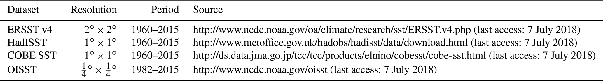
Four globally gridded SST datasets are used in our work (see Table 1): (1) the Hadley Center Sea Ice and Sea Surface Temperature monthly dataset (HadISST) (Rayner et al., 2003); (2) the Centennial In Situ Observation-Based Estimates of the Variability of SST (COBE SST) (Hirahara et al., 2014); (3) Extended Reconstructed Sea Surface Temperature version 4 (ERSST v4) for 1960–2015 (Smith et al., 2008; Huang et al., 2015); and (4) NOAA OISST v2 for 1982–2015 (Reynolds et al., 2007).
2.2 Methodology
Statistical methods, such as conventional empirical orthogonal functions (EOFs) (Kim et al., 1996; von Storch and Zwiers, 1999), correlation analysis, and linear trend analysis, are employed. The significance of each trend has been tested by the Mann–Kendall test using Sen's slope estimates to quantify trends (Sen, 1968). The tests were stipulated to operate with a probability for a false rejection of the null hypotheses (i.e., zero trend) of 5 %. They are conducted with the implicit assumption that the data are serially independent. There are only weakly correlated but not really independent. Thus, the tests are “liberal”; i.e., they have tendencies for falsely rejecting the null hypothesis too often when it is actually valid (von Storch and Zwiers, 1999). However, since the effect is relatively weak, given the small serial correlations, and since we have no results, which are close to the stipulated critical levels, we proceed as if the serial dependence is not of importance. However, this caveat should be kept in mind when assessing the results.
Currently, more than 100 coastal hydrological stations are operating and monitoring nearshore hydrological conditions. Among these stations, only 26 stations have routinely and continuously recorded since 1960, with a percentage of missing data less than 4 %. Also, these stations have undergone only a few (five or fewer) documented relocations. The locations of the 26 coastal hydrological stations are shown in Fig.1a. Due to the fact that this area between 29∘ N (Station 11) and 35∘ N (Station 10) is a vast muddy coast not suitable for hydrological stations, there are only 10 hydrological stations. Among them, some stations were built after the 2000s and some have a high percentage of missing data. That is why no station has been chosen between 29∘ N (Station 11) and 35∘ N (Station 10). Monthly mean SST series were then derived and subjected to a statistical homogeneity test, called the penalized maximum t (PMT) test (more details can be found in Li et al., 2018). Homogenized monthly mean SST series were obtained by adjusting all significant change points that were supported by historic metadata information. These identified change points at each station are displayed in Fig. 1b. The majority of change points are caused by instrument changes and station relocations, accounting for 60.6 % and 24.6 % of the total, respectively. In our work, we consider annual mean values. Some analyses with seasonal mean values are also calculated, but these are not covered by our present account and merely summarized. The supporting evidence is provided in the Supplement.
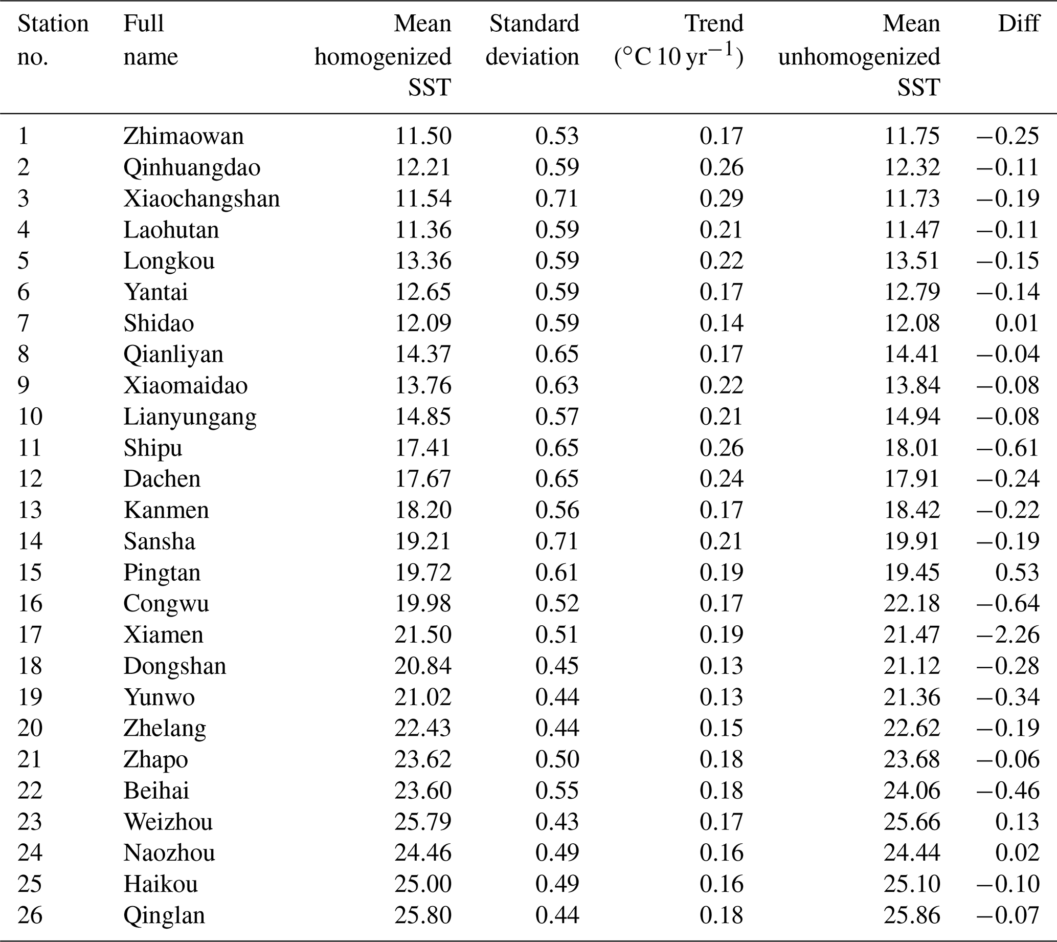
The standard statistics derived from the data in the period of 1960–2015, including the long-term mean, the standard deviation of annual means, and the decadal trends, are listed in Table 2. SSTs vary along the Chinese coast between about 11.5 ∘C at the north and 25 ∘C at the southernmost locations. The standard deviations are of the order of 0.50 ∘C at all locations, with a maximum of 0.71 ∘C and a minimum of 0.43 ∘C. The decadal trends vary between 0.13 and 0.29 ∘C per decade. Table 2 also provides the long-term means of the homogenized data and the raw (unhomogenized) data. The differences between the homogenized data and the raw data (last column) vary between −2.26 and 0.53 K. At 22 of the 26 stations, a downward correction of the mean has been found necessary – only at Station 15 (Pingtan) and Station 23 (Weizhou) was an upward change stipulated, and in two cases there was nearly no change in the mean (at Station 7 – Shidao – and Station 24 – Naozhou).
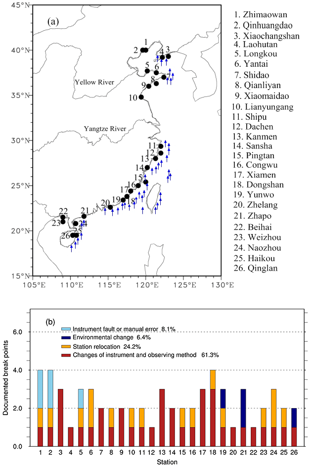
Figure 1Study area and locations of the 26 coastal sites (a) for which continuous monthly SST recordings are available and corrected by eliminating inhomogeneities. The number of identified break points in individual SST stations from 1960 to 2015 (b). Result from Li et al. (2018). Black circles represent the 26 coastal sites and blue arrows represent coastal upwelling.
Table 2Statistics of the time series of the annual homogenized local SST, plus the differences from the raw data, which were used to construct the homogenized series (columns 6 and 7).
The quality of the dataset has already been documented by Li et al. (2018). To add confidence in the quality of this dataset, we compared the new dataset to an independent dataset of local SAT at 26 nearby local stations. Also, this dataset has been homogenized independently of the processing of the SST series. SST and SAT data are not compared directly pairwise but in terms of the patterns and coefficient time series (principal components, or PCs) of their EOFs. The similarity of the principal components is striking. The first PCs share a correlation coefficient of 0.97 and the second 0.86 (Fig. A1 in the Appendix). Thus, the SST series are fully consistent with these SAT series. When this exercise is repeated with CRU TS 3.24.01 instead of the in situ SAT series, we find a similar consistency (see Fig. S1 in the Supplement). The PCs of SAT from CRU also show high correlations of 0.94 and 0.83 with the in situ SST (see Fig. S1) (more details are shown in Appendix A and B). Thus, we conclude that our homogenized SST data are superior to earlier data on SST variability and trends along the Chinese coast.
Given the consistency of the newly homogenized SST series with independent regional SAT data, we use it as a benchmark for assessing the regional quality of the four globally gridded SST datasets in Table 1. In the following, we name the new dataset the “local homogenized SST” with the abbreviation “LH”, while the data extracted from the gridded SST datasets are referred to as the “localized analysis data” with the abbreviation “LA”. For instance, LA-HadISST is the SST found in HadISST in the local grid box, which contains the locations in the LH dataset.
These localized time series (LA) of the three gridded datasets, which extend to the full time window 1960–2015 (ERSST, HadISST, COBE SST; referred to as LA-ERSST, LA-HadISST, and LA-COBE SST), are then compared to the local series (LH) by first comparing the standard deviations and the trends. Calculating from the trends, we then determine differences (Diff) and the root mean square errors (RMSEs) for the 26 stations (Table 3). We do this for annual mean values. The fourth dataset, OISST data, covers a shorter time window from 1982–2015 and has a high spatial resolution. It is used in the concluding section (Sect. 5) to clarify some additional aspects.
For summarizing the results, we compute EOFs of the LH and the LAs, as well as the differences of LH and LAs. The LH data are derived from observational stations, whereas the LA data represent area values averaged across a grid box. Therefore, the LA data should vary less than the LH data. Possible mismatches between the local LH data and the spatial averages of grid box data in the LAs may be related to small-scale effects; however, the usage of EOFs is expected to reduce these truly local specifics, as the first EOFs describe joint covariations among the 26 elements in both the LA and LH datasets.
4.1 Comparing with HadISST
The 56-year mean values of local SST in the analysis LA-HadISST are in all cases higher than at the local stations (Table 3). Some differences are of the order of 2 K and even 3 K, in particular along the East China Sea extending from Station 11 (Shipu) to Station 20 (Zhelang). To some extent, this difference may reflect differences between the averages of a larger coastal ocean area and in situ observations, but not entirely.
The variations in LA are similar to LH, but there are some differences: as expected, 65.4 % of the standard deviations (17) are larger for LH, and in 34.6 % of the cases (9) they are smaller. The correlations are all large enough to reject the null hypothesis of the absence of a link (if we assume serially independence; the 90 % critical value is 0.22) except for the northernmost Station 19 (Yunwo). Part of the difference from the ideal value of 1 may be due to the different spatial scale, but values as low as 0.41 indicate more systematic differences. The trends are positive for all sites (Table 3) – only the northernmost Station 1 (Zhimaowan) signals a weak downward trend in the LA-HadISST dataset. In about 50 % of the cases, the coastal sea warms faster according to LH than to LA-HadISST, and for 50 % it is the opposite. For the two northernmost sites, Station 1 (Zhimaowan) and Station 2 (Qinhuangdao), the warming according to LA is very weak, whereas along the stretch from Station 15 (Pingtan) to Station 19 (Yunwo) the warming according to LA-HadISST is considerably stronger than in LH.
The time series for the two northern sites in the Bohai Sea are shown in Fig. 2. The sequences of maxima and minima share some similarity, but the trends differ markedly. The LH curves (red lines) both exhibit a steady increase, whereas the LA-HadISST curves (black lines) tend to decline in the first 10–20 years and to vary at a mostly constant level (Fig. 2a and b). In this case, the “story told” by LH is considerably different than that of LA-HadISST.
The time series of the SST averaged across the stations from Station 15 (Pingtan) to Station 19 (Yunwo) along the East China Sea coast, where LA-HadISST indicated a stronger warming than in the LH, is shown in Fig. 2c. The local data indicate markedly lower temperatures, which may be mainly because of coastal upwelling (the effect of upwelling will be discussed in Sect. 5), but also other local effects, including local tidal mixing, ocean fronts, seawater vertical mixing, and freshwater discharge, show a weaker trend (0.18 ∘C per decade) than in LA-HadISST (0.35 ∘C per decade).
Table 3Statistics of the time series of the localized SST analysis (LA-HadISST) data series at the 26 stations, as well as the differences (Diff) between statistics of the LH series given in Table 1. The correlation coefficients between LH and LA-HadISST are also calculated (the 90 % confidence level is 0.22, without considering serial correlation). Bold numbers indicate that the correlation coefficients do not conflict with the null hypothesis of no correlation.
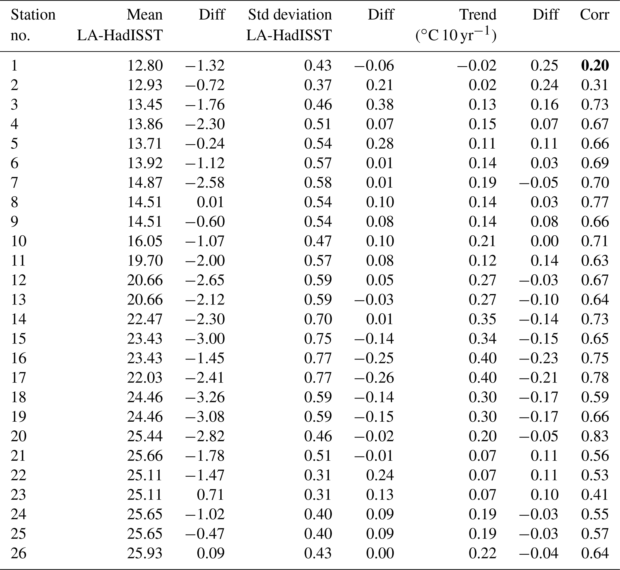
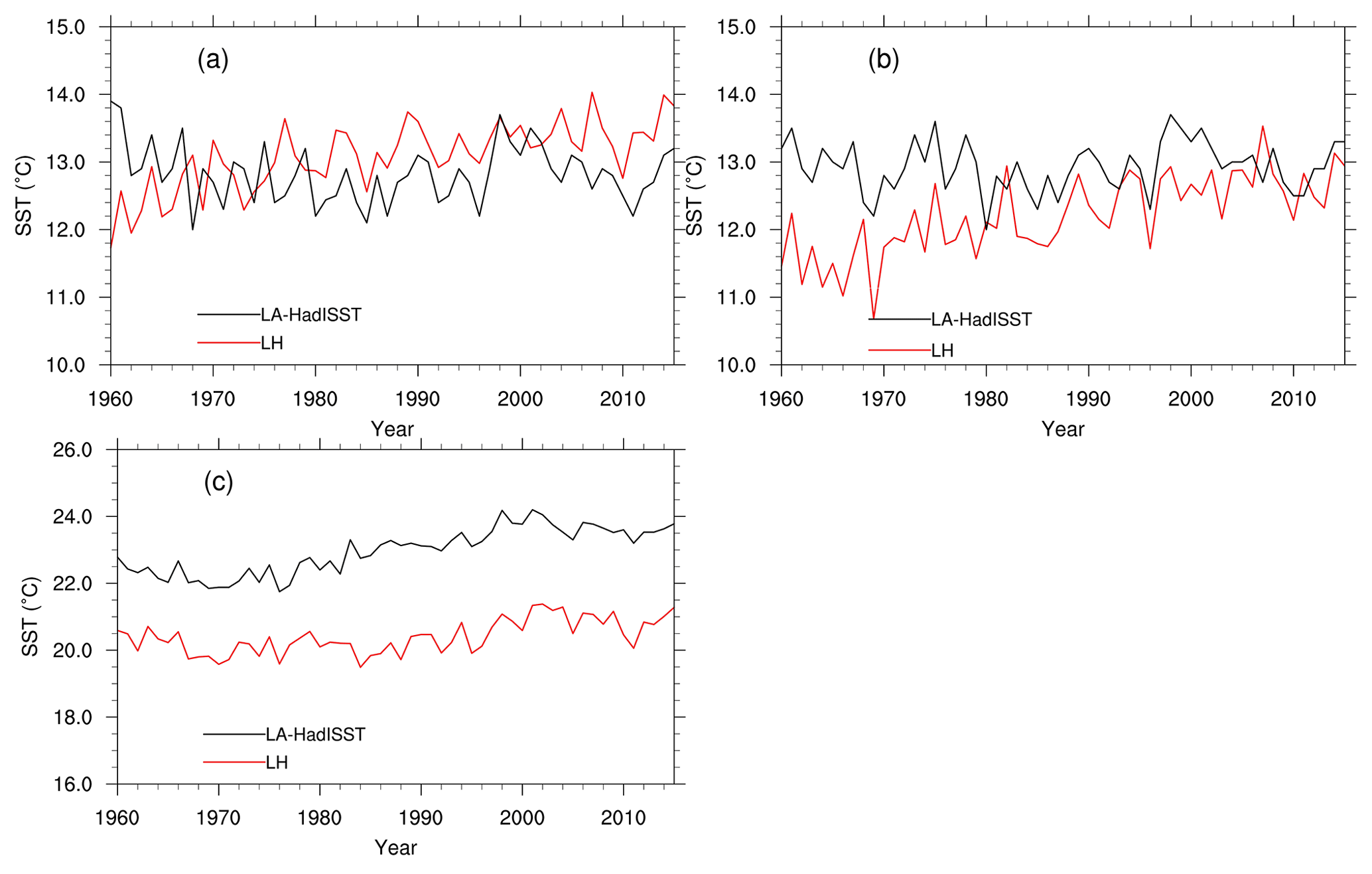
Figure 2The annual mean SST series of LA-HadISST (black line) and LH (red line) from Station 1 (Zhimaowan) (a) and Station 2 (Qinhuangdao) (b). The average annual mean SST series of LA-HadISST (black line) and LH (red line) from Station 15 (Pingtan) to Station 19 (Yunwo) (c).
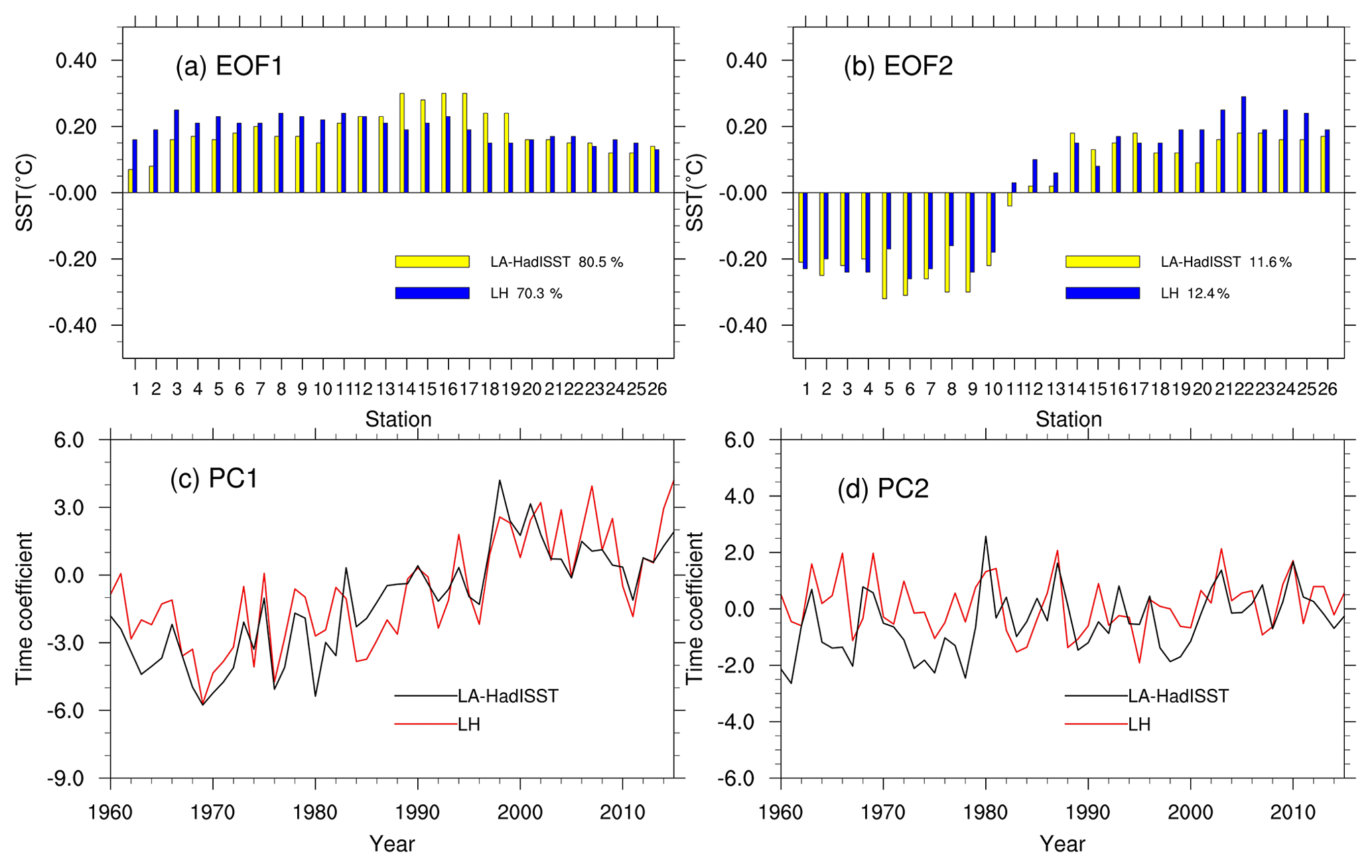
Figure 3Comparison of the EOF1 and EOF2 derived from the LH dataset of local SST at 26 sites (blue bars; red lines) and derived from the localized analysis data LA-HadISST (yellow bars; black lines). (a, b) EOF spatial patterns, (c, d) principal components (time coefficients).
The first two EOFs of the LH and the LA dataset have similar patterns, namely a uniform sign along the entire coast in EOF1, with similar intensities and a north–south dipole (Bohai Sea and Yellow Sea vs. East and South China Sea) in EOF2, as well as a sign change at Station 11 (Shipu) (Fig. 3a and b). The two patterns of LH explain less variance, namely 82.9 % of the total variance, than the LA-HadISST EOFs, which explains 92.9 %. This may be related to the larger spatial variability in local data compared to gridded data. In EOF1, again Station 1 (Zhimaowan) and Station 2 (Qinhuangdao) in the Bohai Sea contribute less in LA-HadISST, whereas Station 15 (Pingtan) to Station 19 (Yunwo) contribute more to the overall warming in LA-HadISST than in LH.
The time coefficients (PCs) are broadly similar, even if the correlations are not very strong: only 0.84 and 0.42 (Fig. 3c and d). A general warming is associated with EOF1 and mostly stationary interannual variability with EOF2. Again, the sequence of maxima and minima is qualitatively similar, but PC2 of LA-HadISST exhibits a break point at about 1980 – interestingly the time when satellites became routinely available for global analyses. These data improve SST sampling, especially in the Southern Ocean and coastal areas (Smith et al., 2008; Lima and Wethey, 2012). Before 1980, PC2 of LH and LA-HadISST differed by about 0.2 (Fig. 3d; this corresponds to a mean difference of 0.04 K at the southern stations from Station 11 to Station 26 during that time and a mean difference 0.04 K at the northern stations from Station 1 to Station 10; Fig. 3b).
To further study the differences in trends, EOFs were calculated from the difference time series, that is, LH anomalies minus LA-HadISST anomalies at the 26 sites (Fig. 4). The first two EOFs account for 31.2 % and 27.6 % of the variance. These numbers are not very different, and their closeness may be indicative that the EOFs are inaccurate (von Storch and Zwiers 1999). These EOFs describe covariations of the differences along long stretches of the coast; in the case of EOF1, this is true for all stations to southern Station 11 (Shipu), i.e., in the East and South China Sea (Fig. 4a). In EOF2 it is true for all stations south of Station 13 (Kanmen), mostly in the Yellow Sea and Bohai Sea (Fig. 4b). PC1 seems to describe a change point at about 1980, whereas PC2 describes a slight upward trend: the differences tend to be larger in earlier years and are almost zero at the end of the considered time interval. That is, in recent years, there have been few differences between LA-HadISST and LH, which is not surprising given better observational and reporting practices.
That in early years inhomogeneities impacted the quality of SST analyses is also not surprising, but it is valuable to learn when these inhomogeneities took place and which time periods in the analyses should be taken with some reservation. Of course, this assertion depends on the assumption that the homogenization of the local data removed all change points and other inhomogeneities.
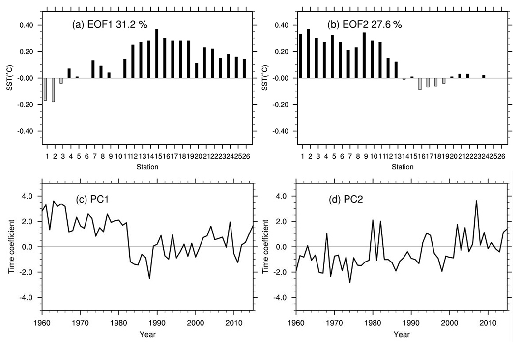
Figure 4The first two EOFs of the difference time series LH–LA-HadISST. (a, b) EOF spatial patterns, (c, d) principal components (time coefficients).
4.2 Comparing with COBE SST
In this subsection, we consider localized SST derived from the LA-COBE SST dataset during 1960–2015. Again, LA-COBE SST is at almost all sites higher than the local data, namely at 21 out of 26 sites. The differences are up to 3 K and again mostly along the East China Sea coast from Station 11 (Shipu) to Station 20 (Zhelang) (see Table S1 in the Supplement). The local correlations are relatively high, namely between 0.55 and 0.85.
The EOFs derived from LA-COBE SST, with the same grid resolution of 1∘ and the same time window of 1960–2015 as LA-HadISST, exhibit broadly the same pattern in space and time as the EOFs of the LH data. Also, the explained variances are close (Fig. S2). The northern stations contribute more to the overall warming represented by EOF1, whereas the stations along the South and East China Sea contribute less. Again, the two northernmost stations, Station 1 (Zhimaowan) and Station 2 (Qinhuangdao), exhibit some systematic differences both in EOF1 and EOF2. The PCs have correlations of 0.80 for EOF1 and 0.50 for EOF2. COBE SST does not capture the recovery of the dip in warming since about 2000, as LH and HadISST did, while EOF2 reveals some warming in the final years. During the 1960s some differences prevail.
Figure 5 shows the EOFs of the difference time series between LH anomalies and LA-COBE SST anomalies. The first EOF dominates, with 49.8 %, whereas the second one represents a share of 17.5 %. The first EOF points to several inhomogeneities, with two prolonged intervals during which LH is higher than LA-COBE SST (i.e., 1960–1978 and 1995–2005), and a strong drop-down to negative PC values after about the year 2005. PC2, on the other hand, appears as mostly stationary, except for a suspiciously negative episode in the early 1960s.
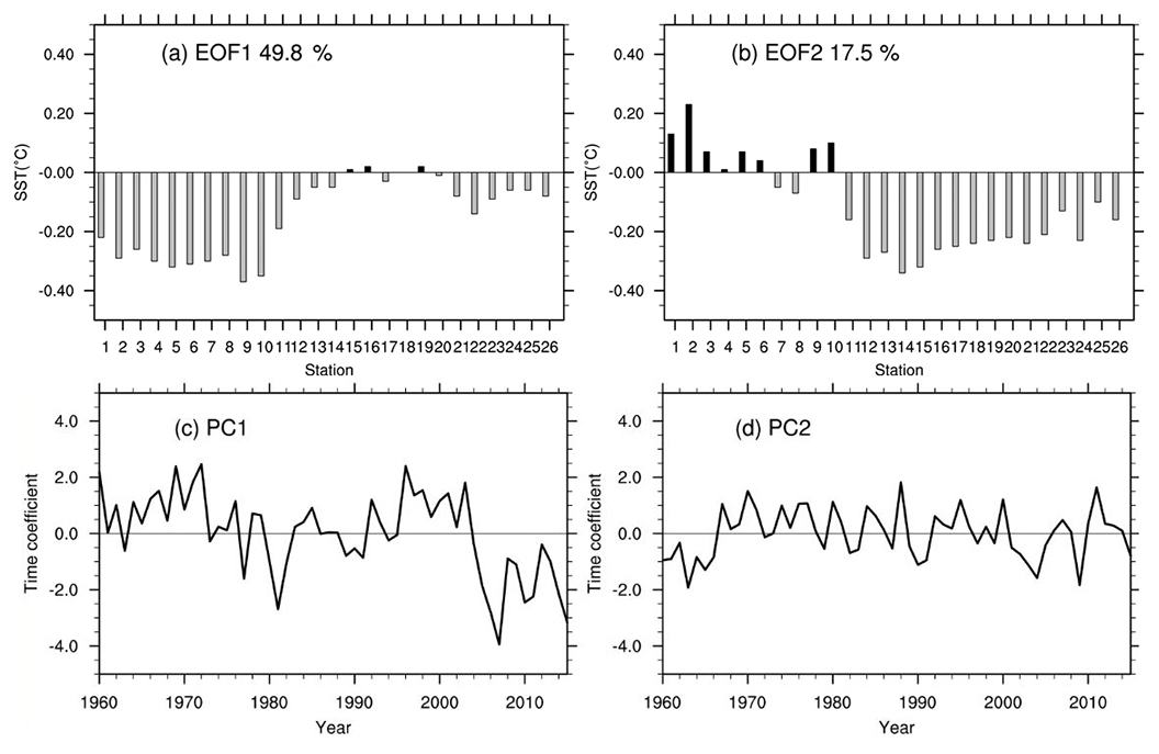
Figure 5EOF analysis of the differences for LH–LA-COBE: (a, b) EOF spatial patterns (EOFs), (c, d) principal components (time coefficients).
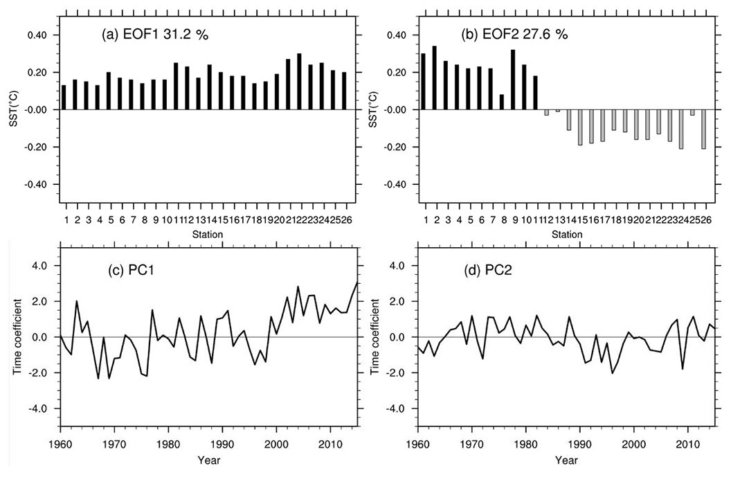
Figure 6EOF analysis of the differences for LH–LA-ERSST: (a, b) EOF spatial patterns (EOFs), (c, d) principal components (time coefficients).
4.3 Comparing with ERSST
ERSST presents SST on a coarser grid compared to the two cases before. Again, the temperatures given by ERSST, as was the case with the other two analyses, are higher than the temperatures recorded at the local sites along the coast (see Table S2). The differences are up to 4 K, and the largest differences are found in the East China Sea from Station 11 (Shipu) to Station 20 (Zhelang). That the differences are in this case even larger than in the other LA cases may be related to the 2∘ coarse resolution of ERSST.
The variability according to ERSST is quite similar to that of LH, at least in terms of EOFs (see Fig. S3). The correlation of the PC1 is 0.83 and of PC2 0.60. LA-HadISST is 0.84 and 0.42, and LA-COBE SST is 0.80 and 0.50. The local correlations vary between 0.37 and 0.82. Again, EOF1 indicates an overall warming and EOF2 indicates interannual variability, with hardly a trend. The relative contributions of the two EOFs compare well to the LH EOFs. In detail, the northernmost stations appear stronger in the EOF1 of LA-ERSST than in that of LH, whereas the northern sites are underrepresented and the southern overrepresented in EOF2.
The EOFs of the differences between LH anomalies and LA-ERSST anomalies are shown in Fig. 6. They differ strongly from those found for LA-COBE SST and LA-HadISST. The first EOF differences resemble the first EOFs of LH and LA-ERSST (not shown; see Fig. S3) – the long-term trend in LA-ERSST is smaller than in the local data – everywhere. The second EOF is again a dipole pattern, with the Bohai Sea and the Yellow Sea on the one side and the East China Sea and South China Sea on the other. The time series of PC2 fluctuates around zero without a prominent long-term trend.
We have mainly examined three global gridded analysis SST datasets in Chinese coastal waters. For doing so, we have compared a number of statistical properties for 26 coastal hydrological locations as given by the analyses and by a newly digitized and homogenized dataset (Li et al., 2018). For demonstrating the utility of the local dataset, we have compared the local SST series (named LH) with independent local homogenized SAT data from nearby meteorological stations. The variations of the two series are fully consistent. Another argument points to the quality of the LA dataset in that the differences between LH and the three LAs (localized data from the different global analyses: HadISST1, COBE SST, ERSST) considered are not uniform (except for the time mean); instead, the LAs deviate in different ways from LH. If this were not the case, one could be tempted to argue that the differences are manifestations of inefficiencies in the LH dataset. This is not the case.
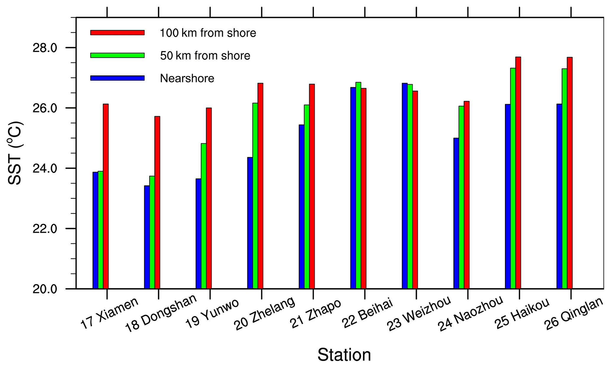
Figure 7Simulated SSTs at different distances from each coastal hydrological station in the South China Sea.
In this study, we found that all of these globally gridded datasets exhibit surface temperatures usually higher than the LH data, especially in the East China Sea. This difference may be caused by two factors. In the China seas, most of the coastal upwelling currents occur at the East China Sea and the northern South China Sea, with other small upwelling currents at the tops of the Liaodong Peninsula and Shandong Peninsula (Fig. 1) (Yan, 1991). The consensus of previous studies is that coastal upwelling currents result in cooling SST at these coastal areas (Xie et al., 2003; Guan et al., 2009; Su et al., 2012). In our study, we find that in situ shoreline SSTs at the upwelling areas (e.g., Station 4 – Laohutan, Station 11 – Shidao, and Station 18 – Dongshan) are always colder than global gridded SST data, with values below −1 K (Tables 2, 3, and S1).
We hypothesize that these negative differences are connected by coastal upwelling currents. To test this hypothesis, we examine the output of a numerical simulation of the currents in the South China Sea with a grid resolution of 0.04∘. The model is embedded in an almost global model with 1∘ grid resolution (Tang et al., 2018). The model used here is the Hybrid Coordinate Ocean Model (HYCOM) that is exposed to periodic climatological atmospheric forcing, with a fixed annual cycle but no weather disturbances. The atmospheric forcing comes from the International Comprehensive Ocean–Atmosphere Data Set (ICOADS). We extract simulated SSTs at three different distances (i.e., near the station, 50 km, and 100 km from each coastal hydrological station in South China Sea). Figure 7 shows that most shoreline SSTs are lower than ambient offshore SSTs, especially SSTs at 100 km from the shoreline. However, Station 22 (Beihai) and Station 23 (Weizhou) are not affected by coastal upwelling, and, consistently, there are no notable differences among SSTs at three different distances from the two stations. The result reflects the fact that the homogenized SST dataset for shoreline stations catches this relative cooling water effect of the regional upwelling currents. On the other hand, the global gridded SST datasets point to higher temperatures, which may be caused by their coarse resolution. The differences are largest in the case of the coarsest analysis (ERSST) but weakest in the OISST v2 analysis with a resolution of 0.25∘ (Fig. 8; see below; note that the difference of LH minus LA-OISST is restricted to the warmer episode during 1982–2015). Meanwhile, the lack of nearshore observations when compiling nearshore box averages in coastal areas may also cause these differences (Wang et al., 2018). There also some other local mechanisms with a smaller scale that can cause cooling water in the China seas, such as the China coastal current (CCC) (Belkin and Lee, 2014) and ocean fronts (Zhao, 1987; Hickox et al., 2000), related to which a shallow water shelf front and estuarine plume front are two major fronts in the Bohai Sea and the Yellow Sea in summer. A coastal current front, an upwelling front, and a strong westerly boundary current usually appear in the East China Sea and the South China Sea, which may also be related to coastal upwelling currents.

Figure 8The mean SST differences at the 26 locations between LH and LA-OISST (1982–2015; red line), LH and LA-ERSST (1960–2015; blue line), LH and LA-COBE SST (1960–2015; green line), and LH and LA-HadISST (1960–2015; black line).
In summary, our main results are as follows.
-
The mean SST in LH at many sites is considerably lower than that in the LA datasets. We suggest that this is related to local oceanic effects, such as coastal upwelling. The LA datasets cannot catch this cooling effect of the regional upwelling currents well. On the other hand, the global gridded SST datasets point to higher temperatures, which may be caused by their coarse resolution when averaging in the LA datasets. However, systematic differences would not be expected to strongly influence the overall variability and trends.
-
The first EOF in all datasets indicates a general warming, and the second indicates interannual variability. This is true not only in the local LH data but also in all globally gridded LA datasets.
-
In the years following the introduction of satellites in monitoring SST, since about 1980, the different global analyses converge, and the differences from the local dataset become smaller. In support of this, the comparison with the high-resolution analysis OISST v2 for the post-satellite period 1982–2015 reveals few differences (not shown; see Fig. S4).
-
In the years before 1980, some noteworthy differences are found. The differences between the LH data anomalies and the LA data anomalies are nonuniform across the different LA datasets. For instance, for ERSST the long-term trends differ; in the case of COBE SST several jumps emerge, and in the case of HadISST, a jump is found at the time of the advent of routine satellite data, along with a trend in the PC2 of the differences.
Thus, our overall conclusion is that the global gridded SST datasets correctly describe the main features of variabilities and trends in regional waters, but significant improvements in the regional analyses may be gained when quality-controlled homogenized data are incorporated. In particular, for the time prior to the usage of remote sensing by satellites and in regions where observational efforts have been limited, such efforts are valuable contributions to climate variability and change studies. Our example should also be an encouragement for national climate services to revisit regional data and to invest in the elimination of inconsistencies caused by inhomogeneities. There are projects and research dedicated to the quality control and homogenization of in situ data (Kuglitsch et al., 2012; Hausfather et al., 2016; Minola et al., 2016). It is useful to keep some high-quality data separate from those available for analyses for validation activities such as our work and the work of others (Hausfather et al., 2017).
When this exercise is repeated with CRU TS 3.24.01 instead of the in situ SAT series, we find similar consistency (see Fig. S1). The PCs of SAT from CRU also show high correlations of 0.94 and 0.83 with the in situ SST (see Fig. S1).
We conclude that the two datasets are consistent; the first EOFs describe the warming of recent decades, and the second EOFs describe interannual variability and may be influenced by ENSO and other patterns of natural variability. We furthermore conclude that the new description of SST variability and trends at the 26 sites along the Chinese coast presents a reliable account of the past since 1960 and may thus serve as a benchmark for assessing global analyses of SST datasets.
All four gridded SST analyses used in this study are publicly available and can be downloaded freely from the websites shown in Table 1. The observational in situ SST data from the coastal stations and the coordinates of coastal stations can be obtained from the National Marine Science Data Center, National Science and Technology Resource Sharing Service Platform of China (http://mds.nmdis.org.cn, last access: 8 July 2018). However, observational in situ SST data from only nine coastal stations are publicly available. SST data from the rest of the stations can be obtained by application on the website.
The supplement related to this article is available online at: https://doi.org/10.5194/os-15-1455-2019-supplement.
HS contributed to the design and the implementation of the processing chain. YL undertook the data analysis and produced the figures with contributions from QW. HS and YL led the writing process. ST ran the HYCOM model. QZ contributed to the surface air temperature collection.
The authors declare that they have no conflict of interest.
This work is funded by a program of the National Natural Science Foundation of China (no. 41376014; no. 41706020), the National Key Research and Development Program of China (no. 2018YFA0605603; no. 2017YFC1404700), and also supported by the Hamburg University Cluster of Excellence CliSAP in Germany; Shengquan Tang's work is funded by the Chinese Scholarship Council.
This research has been supported by a program of the National Natural Science Foundation of China (grant nos. 41376014 and 41706020) and the National Key Research and Development Program of China (grant nos. 2018YFA0605600 and 2017YFC1404700).
This paper was edited by Markus Meier and reviewed by Igor Belkin and two anonymous referees.
Belkin, I. M.: Rapid warming of Large Marine Ecosystems, Prog. Oceanogr., 81, 207–213, 2009.
Belkin, I. M. and Lee, M.-A.: Long-term variability of sea surface temperature in Taiwan Strait, Clim. Change, 124, 821–834, 2014.
Burrows, M., Schoeman, D., Buckley, L., Moore, P., Poloczanska, E., Brander, K., Brown, C., Bruno, J., Duarte, C., Kiessling, W., O'Connor, M., Pandolfi, J., Parmesan, C., Schwing, F., Sydeman, W., and Richardson, A.: The pace of shifting climate in marine and terrestrial ecosystems, Science, 334, 652–655, 2011.
Guan, J., Cheung, A., Guo, X., and Li, L.: Intensified upwelling over a widened shelf in the northeastern South China Sea, J. Geophys. Res., 114, https://doi.org/10.1029/2007JC004660, 2009.
Harris, I., Jones, P. D., Osborn, T. J., and Lister, D. H.: Updated high-resolution grids of monthly climatic observations – the CRU TS3.10 dataset, Int. J. Climatol., 34, 623–642, 2014.
Hausfather, Z., Cowtan, K., Menne, M. J., and Williams Jr., C. N.: Evaluating the impact of U.S. Historical Climatology Network homogenization using the U.S. Climate Reference Network, Geophys. Res. Lett., 43, 1695–1701, 2016.
Hausfather, Z., Cowtan, K., Clarke, D., Jacobs, P., Richardson, M., and Rohde, R.: Assessing recent warming using instrumentally homogeneous sea surface temperature records, Sci. Adv. 3, e1601207, https://doi.org/10.1126/sciadv.1601207, 2017.
Hickox, R., Belkin, I. M., Cornillon, P., and Shan, Z.: Climatology and seasonal variability of ocean fronts in the East China, Yellow and Bohai seas from satellite SST data, Geophys. Res. Lett., 27, 2945–2948, 2000.
Hirahara, S., Ishii, M., and Fukuda, Y.: Centennial-Scale Sea Surface Temperature Analysis and Its Uncertainty, J. Climate, 27, 57–75, 2014.
Honkoop, R. J. C., der Meer, J., Van Beukema, J. J., and Kwast, D.: Does temperature-influenced egg production predict the recruitment in the bivalve Macoma Balthica?, Mar. Ecol. Prog. Ser., 64, 229–235, 1998.
Huang, B., Banzon, V., Freeman, J., Lawrimore, J., Liu, W., Peterson, T., Thorne, P., Woodruff, S., and Zhang, H.: Extended Reconstructed Sea Surface Temperature version 4 (ERSST v4), Part I: Upgrades and intercomparisons, J. Climate, 28, 911–930, 2015.
Ishii, M., Shouji, A., Sugimoto, S., and Matsumoto, T.: Objective analyses of sea-surface temperature and marine meteorological variables for the 20th century using ICOADS and the Kobe Collection, Int. J. Climatol., 25, 865–879, 2005.
Kim, K. Y., North, G. R., and Huang, J. P.: EOFs of one dimensional cyclostationary time series: Computation, examples, and stochastic modeling, J. Atmos. Sci., 53, 1007–1017, 1996.
Kuglitsch, F. G., Auchmann, R., Bleisch, R., Bronnimann, S., Martius, O., and Stewart, M.: Break detection of annual Swiss temperature series, J. Geophys. Res., 117, 1–12, 2012.
Li, Y., Mu, L., Liu, Y. L., Wang, G. S., Zhang, D. S., Li, H., and Han, X.: Analysis of variability and long-term trends of sea surface temperature over the China Seas derived from a newly merged regional data set, Clim. Res., 73, 217–231, 2017.
Li, Y., Wang, G. S., Fan, W. J., Liu, K. X., Wang, H., Tinz, B., von Storch, H., and Feng, J. L.: The homogeneity study of the sea surface temperature data along the coast of the China Seas, Ac. Ocean. Sin., 40, 17–28, 2018 (in Chinese but with English abstract).
Lima, F. P. and Wethey, D. S.: Three decades of high-resolution coastal sea surface temperatures reveal more than warming, Nat. Commun., 3, 704, https://doi.org/10.1038/ncomms1713, 2012.
Liu, Q. Y. and Zhang, Q.: Analysis on long-term change of sea surface temperature in the China Seas, J. Ocean University China, 12, 295–300, 2013.
Mantua, N. J. and Hare, S. R.: The Pacific decadal oscillation, J. Oceanogr., 58, 35–44, 2002.
Minola, L., Azorin-Molina, C., and Chen, D. L.: Homogenization and assessment of observed near-surface wind speed trends across Sweden, 1956–2013, J. Climate, 29, 7397–7415, 2016.
Rayner, N. A., Parker, D. F., Horton, E. B., Folland, C., Alexander, L., Rowell, D., Kent, E., and Kaplan, A.: Global analyses of sea surface temperature, sea ice, and night marine air temperature since the late nineteenth century, J. Geophys. Res., 108, 1063–1082, 2003.
Reynolds, R. W., Smith, T. M., Liu, C. Y., Chelton, D. B., Casey, K. S., and Schlax, M.: Daily high-resolution-blended analyses for sea surface temperature, J. Climate, 20, 5473–5496, 2007.
Saji, N. H., Goswami, B. N., Vinayachandran, P. N., and Yamagata, T.: A dipole mode in the tropical Indian Ocean, Nature, 401, 360–363, 1999.
Sen, P. K.: Estimates of regression coefficient based on Kendall's tau, J. Am. Stat. Assoc., 63, 1379–1389, 1968.
Smith, T. M., Reynolds, R. W., Peterson, T. C., and Lawrimore, J.: Improvements to NOAA's historical merged land-ocean surface temperature analysis (1880–2006), J. Climate, 21, 2283–2296, 2008.
Su, J., Xu, M., Pohlmann, T., Xu, D., and Wang, D.: A western boundary upwelling system response to recent climate variation (1960–2006), Cont. Shelf Res., 57, 3–9, 2012.
Tang, S., von Storch, H., Chen, X., and Zhang, M.: “Noise” in climatologically driven ocean models with different grid resolution, Oceanologia, 61, 300–307, https://doi.org/10.1016/j.oceano.2019.01.001, 2019.
Tokinaga, H., Xie, S. P., Deser, C., Kosaka, Y., and Okumura, Y. M.: Slowdown of the Walker circulation driven by tropical Indo-Pacific warming, Nature, 491, 439–443, 2012.
Vecchi, G. A., Clement, A., and Soden, B. J.: Examining the Tropical Pacific's Response to Global Warming, EOS T. Am. Geophys. Un., 89, 81–83, 2008.
von Storch, H. and Zwiers, F. W.: Statistical analysis in climate research, Cambridge University Press, London, 484 pp., 1999.
Wang, Q. Y., Li, Y., Li, Q. Q., and Wang, Y. N.: A comparison and evaluation of two centennial-scale sea surface temperature datasets in the China Seas and their adjacent sea areas, J. Trop. Meteor., 24, 452–460, 2018.
Wernberg, T., Bennett, S., Babcock, R. C., Bettignies, T., Cure, K., Depczynski, M., Dufois, F., Fromont, J., Fulton, C. J., Hovey, R. K., Harvey, E. S., Holmes, T. H., Kendrick, G. A., Radford, B., Santana-Garcon, J., Saunders, B. J., Smale, D. A., Thomsen, M. S., Tuckett, C. A., Tuya, F., Vanderklift, M. A., and Wilson, S.: Climate-driven regime shift of a temperature marine ecosystem, Science, 353, 169–172, 2016.
Wu, L. X., Cai, W. J., Zhang, L. P., Nakamura, H., Timmermann, A., Joyce, T., McPhaden, M. J., Alexander, M., Qiu, B., Visbeck, M., Chang, P., and Giese, B.: Enhanced warming over the global subtropical west boundary currents, Nat. Clim. Change, 2, 161–166, 2012.
Xie, S. P., Xie, Q., Wang, D., and Liu, W. T.: Summer upwelling in the South China Sea and its role in regional climate variations, J. Geophys. Res., 108, 3261, https://doi.org/10.1029/2003JC001867, 2003.
Xie, S. P., Clara, D., Gabriel, A. V., Ma, J., Teng, H. Y., and Andrew, T. W.: Global warming pattern formation: sea surface temperature and rainfall, J. Climate, 23, 966–986, 2010.
Xu, W. H., Li, Q. X., Wang, X. L., Yang, S., Cao, L. J., and Feng, Y.: Homogenization of Chinese daily surface air temperature and analysis of trends in the extreme temperature indices, J. Geophys. Res., 118, 9708–9720, 2013.
Yan, T. Z.: A preliminary classification of coastal upwellings in the China Seas. Mar. Sci. Bull., 10, 1–6, 1991 (in Chinese with English abstract).
Yeh, S. W. and Kim, C. H.: Recent warming in the Yellow/East China Sea during winter and the associated atmospheric circulation, Cont. Shelf Res., 30, 1428–1434, 2010.
Zhao, B. R., Ren, G. F., Cao, D. M., and Yang, Y. L.: Characteristics of the ecological environment in upwelling area adjacent to the Changjing River Estuary, Ocean. Lim. Sin., 32, 327–333, 2001 (in Chinese with English abstract).
- Abstract
- Introduction
- Data and methodology
- Local homogenized SST records along the Chinese coast
- Comparison with gridded SST datasets in Chinese coastal waters
- Discussion and conclusion
- Data availability
- Author contributions
- Competing interests
- Acknowledgements
- Financial support
- Review statement
- References
- Supplement