2.1 Model configuration and control simulation

We use OTIS to simulate the effects of SLR on the tides around Australia. OTIS is a portable, dedicated, numerical shallow water tidal model which has been used extensively for both global and regional modelling of past, present, and future ocean tides (e.g. Egbert et al., 2004; Pelling and Green, 2013; Wilmes and Green, 2014; Green et al., 2017). It is highly accurate both in the open ocean and in coastal regions (Stammer et al., 2014), and it is computationally efficient. The model solves the linearized shallow-water equations (e.g. Hendershott, 1977) given by

where U is the depth integrated volume transport, which is calculated as tidal current velocity u multiplied by water depth H. f is the Coriolis vector, g denotes the gravitational constant, ζ stands for the tidal elevation with respect to the moving seabed, ζ_SAL denotes the tidal elevation due to ocean self-attraction and loading (SAL), and ζ_EQ is the equilibrium tidal elevation. F represents energy losses due to bed friction and barotropic–baroclinic conversion at steep topography. The former is represented by the standard quadratic law:

where C_d=0.003 is a non-dimensional drag coefficient, and u is the total velocity vector for all the tidal constituents. The parameterization for internal tide drag, ${\mathbf{F}}_w=C\left|\mathbf{U}\right|$, includes a conversion coefficient C, which is defined as (Zaron and Egbert, 2006; Green and Huber, 2013)

Here, γ=50 is a scaling factor, N_b is the buoyancy frequency evaluated at the seabed, $\stackrel{\mathrm{‾}}{N}$ is the vertical average of the buoyancy frequency, and ω is the frequency of the tidal constituent under evaluation. Values of both N_b and $\stackrel{\mathrm{‾}}{N}$ follow from the prescription of horizontally uniform stratification $N\left(z\right)=N_{\mathrm{0}}\exp (-z/\mathrm{1300})$, where $N_{\mathrm{0}}=\mathrm{5.24}\times {\mathrm{10}}^{-\mathrm{3}}$ s⁻¹ has been obtained from a least-squares fit to present-day climatological hydrography (Zaron and Egbert, 2006).

The model solves Eqs. (1)–(1) using forcing from the astronomical tide-generating potential only (represented by ζ_EQ in Eq. 1), with the SAL term being derived from TPXO8 (Egbert and Erofeeva, 2002, updated version). An initial spin-up from rest over 7 days is followed by a further 15 days of simulation time, on which harmonic analysis is performed to obtain the tidal elevations and transport. Here, we investigate the two dominating semi-diurnal and diurnal tidal constituents, M₂ and K₁, respectively. The model bathymetry comes from the ETOPO1 dataset (Amante and Eakins, 2009, see Fig. 1 for the present domain), which was averaged to $\mathrm{1}/\mathrm{20}{}^{\circ }$ horizontal resolution. For the control run with present-day water depths, the domain model heights at the open boundaries were constrained to elevation data from a coarser-resolution global OTIS run, taken from Wilmes et al. (2017). TPXO8 was used to validate the model (alongside tide gauge data at 24 locations); see Sect. 2.4.

2.2 Dissipation computations

The computation of tidal dissipation rates, D, was done following Egbert and Ray (2001):

Here, W is the work done by the tide-generating force and P is the energy flux given by

where the angular brackets mark time averages over a tidal period.

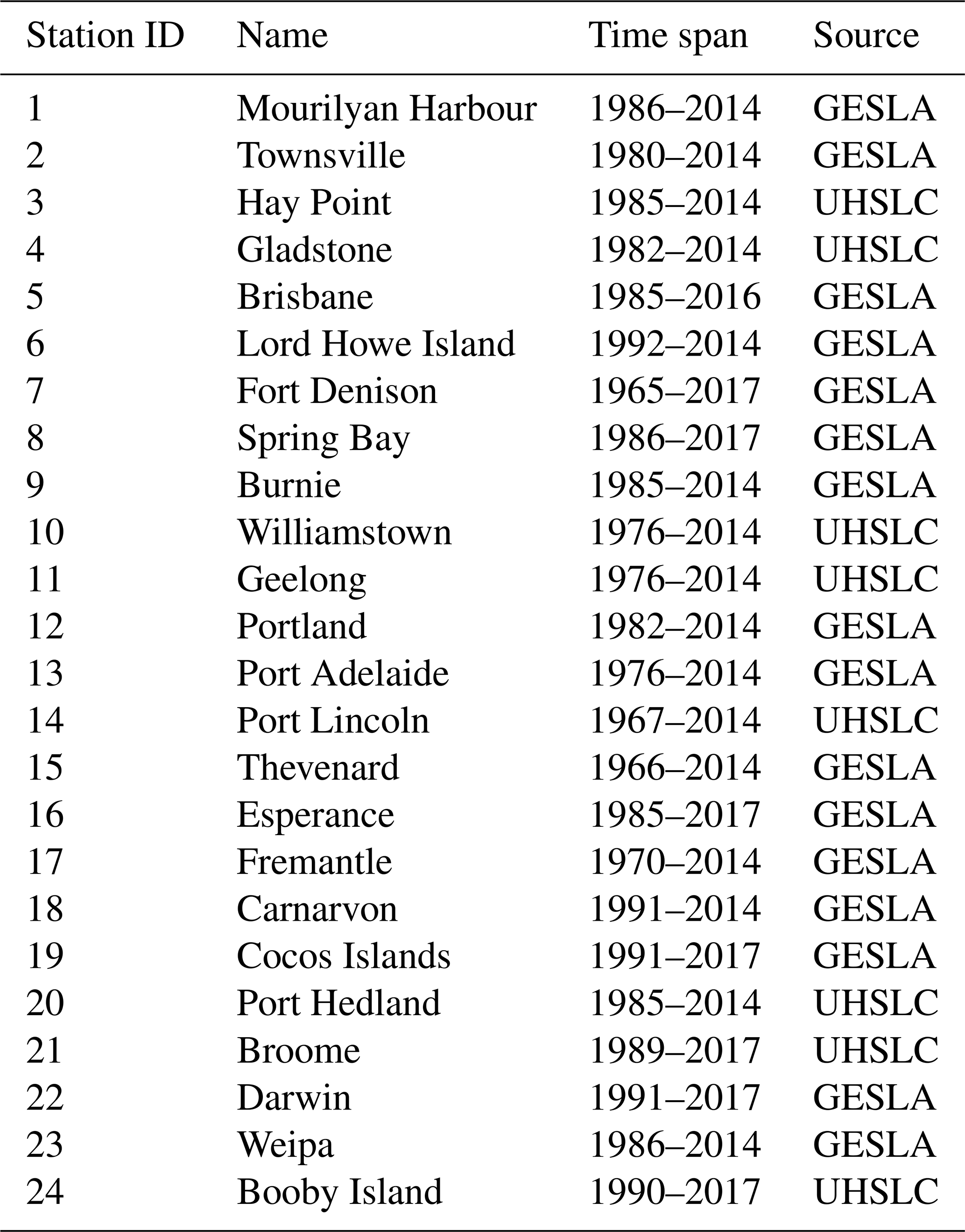
Table 1Start and end dates of the analysed tide gauge records, including names and running index for identification in Fig. 1.

Download Print Version | Download XLSX

2.3 Implementing sea-level rise

The model runs are split into two sets. In the first, we allow low-lying grid cells to flood as sea level rises, whereas in the second set we introduce vertical walls at the present-day coastline. Following Pelling et al. (2013), we denote these sets “flood” (FL) and “no flood” (NFL), respectively. A range of SLR scenarios corresponding to predicted global mean sea-level increases from large-scale ice sheet collapses (Wilmes et al., 2017) are investigated in both sets. This is done via the implementation of a uniform depth increase across the entire domain of 1, 3, 5, 7, and 12 m. Boundary conditions for each of the SLR scenarios are generated from global simulations. The 5, 7, and 12 m SLR NFL runs were taken directly from Wilmes et al. (2017) and the remaining global simulations were carried out following the methodology outlined in Wilmes et al. (2017) but with varying global sea-level changes and allowing for inundation in the FL runs. Additionally, we simulated tidal responses to future changes in water depth extrapolated from geocentric sea-level trend patterns as observed by satellite altimetry (see Carless et al., 2016; Schindelegger et al., 2018). While such projections contain not only the actual long-term trend of sea level but also significant (sub-)decadal variability, little difference was found for tidal perturbations with respect to our uniform SLR scenarios (see the Supplement). It is also unknown how the magnitude and spatial variation of the trend pattern may change over the period of time required to equate a uniform SLR, especially with the larger scenarios considered here. Hence, in the following, the focus is on the uniform SLR scenarios. We choose to show results for the 1 and 7 m SLR simulations because they best exemplify the changes to tidal characteristics across the domain and also correspond to a high but probable level for the end of this century and an extreme case in which large levels of ice sheet collapse has occurred, respectively (e.g. Wilmes et al., 2017). The simulations with 12 m of SLR have little physical justification, but they allow us to assess how any tidal trends seen up to 7 m, if they appear, may evolve for even higher levels of SLR.

2.4 Model validation

For validation of our numerical experiments, time series of hourly sea-level data from 24 stations around Australasia were obtained from the Global Extreme Sea Level Analysis version 2 (GESLA-2; Woodworth et al., 2017) and the University of Hawaii Sea Level Center (UHSLC; Caldwell et al., 2015); see Table 1. With few exceptions, record lengths are short, but all time series span at least 28 years to allow for an appropriate representation of the 18.61-year nodal cycle in lunar tidal constituents (Haigh et al., 2011). Upon removal of years missing more than 25 % of hourly observations, a three-tiered least-squares fitting procedure was applied to (i) extract mean M₂ and K₁ tidal constants of amplitude H and phase lag G, (ii) deduce linear trends in H and G for both constituents over the complete time series at each station, and (iii) estimate the corresponding long-term trend in MSL. A total of 10 out of 24 tide gauge stations yielded statistically insignificant M₂ amplitude trends at the 95 % confidence level and were thus excluded from the model trend validation below; see Fig. 1 for a graphical illustration.

The processing protocol, essentially taken from Schindelegger et al. (2018), is based on a separation of tidal and non-tidal residuals from the longer-term MSL component through application of a 4-day moving average with Gaussian weighting. The high-frequency filter residuals obtained were then harmonically analysed for 68 tidal constituents using the Matlab^® UTide software package (Codiga, 2011), with analysis windows either set to the entire time series (step i) or shifted on an annual basis (step ii). In both cases, we configured UTide for standard least-squares and a white-noise approach in the computation of confidence intervals. Subsequent regressions of annual M₂ tidal constants were performed with a functional model composed of a linear trend, a lag 1-year autocorrelation, AR(1), and sinusoids to account for nodal modulations. Trends in MSL were likewise determined through regression under AR(1) assumptions, upon a priori reduction of the influence of the 18.61-year equilibrium tide.

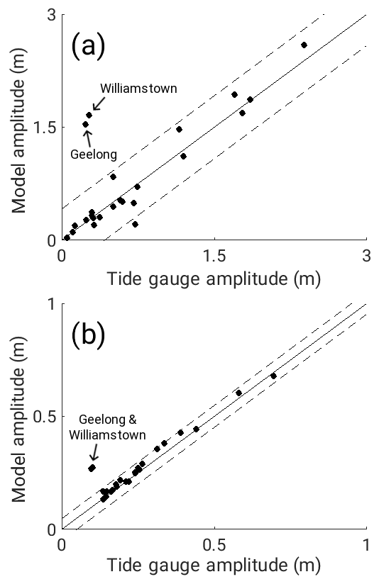
Figure 2The constituent amplitude at each tide gauge position calculated from GESLA and UHSLC data and the model control simulation for (a) M₂ and (b) K₁. The solid line marks the zero difference line. The dashed lines mark 1 standard deviation of the difference.

Download

A regression of the constituent amplitudes calculated from the OTIS control simulation for the present-day bathymetry against the M₂ and K₁ amplitudes from harmonic analysis of the tide gauge data (Fig. 2) reveals that the model performs well at all sample sites except at stations Williamstown and Geelong (see Fig. 1 and Table 1). Here, simulated amplitudes are overestimated by a factor of 5 (M₂) and 2 (K₁), respectively. Both of stations lie on the coast of Port Phillip Bay, a shallow bay isolated from the Bass Strait by two peninsulas. The eastern peninsula is long and narrow, and not resolved in the model bathymetry due to the spatial averaging performed on the source ETOPO1 dataset. As such, the tidal wave from the Bass Strait penetrates into the bay and builds up in amplitude through reflection at lateral boundaries. Excluding Williamstown and Geelong from the comparison, we obtain a root mean square (rms) error for the constituent amplitudes of 17 cm for M₂ and 2 cm for K₁, while correlation coefficients are at 0.97 and 0.99, respectively. Estimates of the median absolute difference between model and test stations can be used to quantify possible biases in a robust way (Stammer et al., 2014); corresponding values are 8 cm for M₂ and 1 cm for K₁ irrespective of whether stations in Port Phillip Bay are included or not. Median phase differences with respect to the tide gauge estimates are 21^∘ for M₂ and 3^∘ for K₁. These statistics give confidence in the model's accuracy and in the assertion that areas where the disagreement between model and tide gauge data is largest are where the resolution of the model has not resolved fine-structure coastal features.

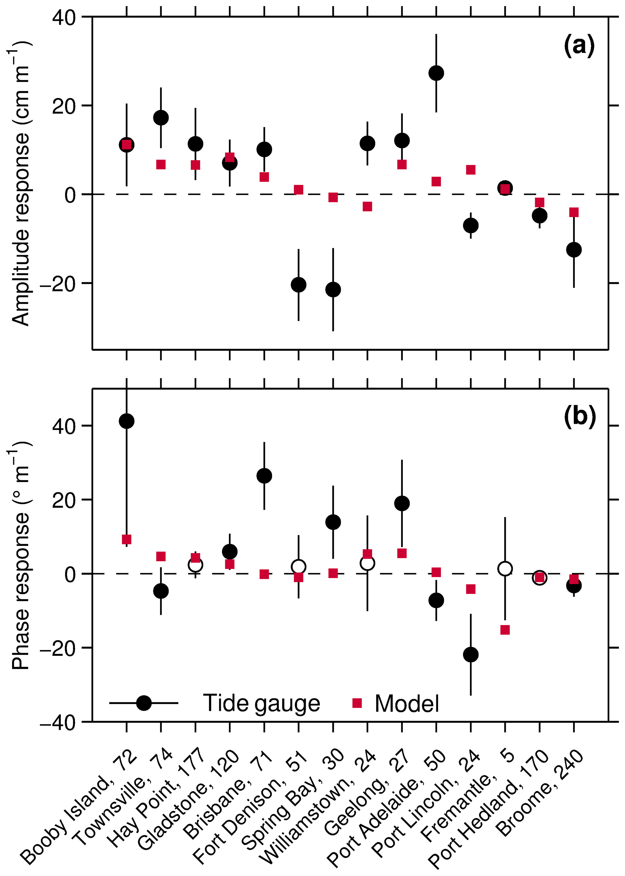
Figure 3Observed and modelled M₂ response coefficients in (a) amplitude H and (b) phase lag G per metre of SLR. Model values (red squares) are based on the 1 m FL simulations, while tide gauge estimates at 14 out of 24 locations are shown in black. Error bars correspond to 2 standard deviations, propagated from the trend analyses of sea-level and annual tidal estimates of M₂. Stations with insignificant phase trends (at the 95 % confidence level) are shown as white markers in panel (b). Numbers at the end of the station labelling indicate mean observed M₂ amplitudes (cm).

Download

Additional comparisons with gridded M₂ data were performed using the TPXO8 inverse solution, linearly interpolated to the grid of the model domain (see http://volkov.oce.orst.edu/tides, last access: 17 April 2018, for details). The rms difference between the model and the TPXO8 data is 7 cm for M₂ and 2 cm for K₁. The variance capture (VC) of the control was also calculated to see how well the overall character of the tidal constituents was represented (e.g. Pelling and Green, 2013):

where RMSD is the rms difference between the control simulation and TPXO8, and S denotes the rms standard deviation of the TPXO8 amplitudes. The VC is above 96 % for M₂ and 97 % for K₁.

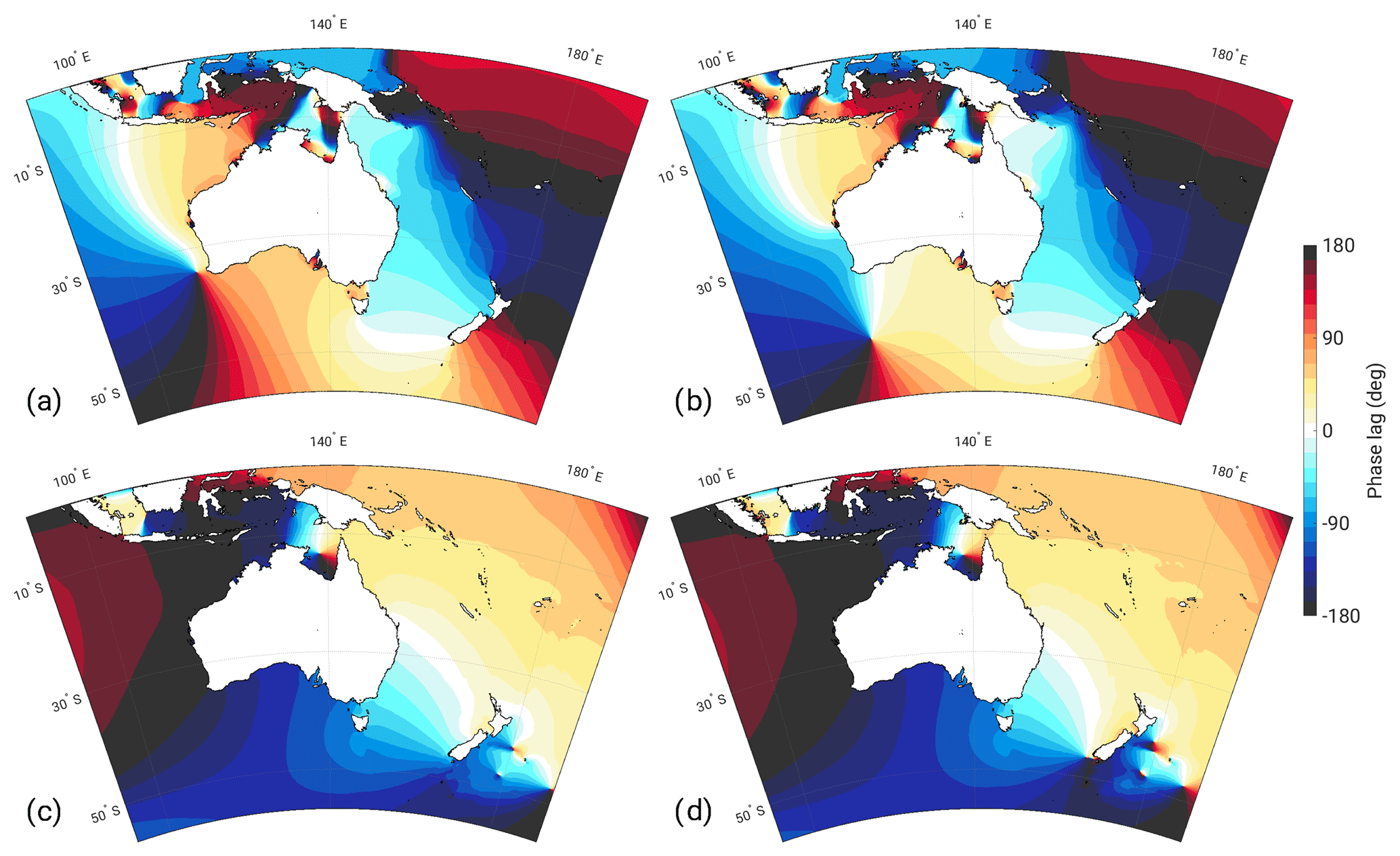
Figure 4The constituent phase lags with respect to the Greenwich meridian (^∘) for the control (a, c) and 7 m SLR (b, d) simulations for M₂ (a, b) and K₁ (c, d).

Download

For validation of the simulated M₂ changes under SLR, we followed Schindelegger et al. (2018) and condensed measured M₂ trends (∂H, ∂G) and MSL rates (∂s) to response coefficients in amplitude $(r_H=\partial H/\partial s)$ and phase $(r_G=\partial G/\partial s)$. Simulated amplitude and phase changes from the 1 m FL run at the location of 14 tide gauges were interpolated from nearest-neighbour cells and also converted to ratios of r_H and r_G. Graphical comparisons in Fig. 3 indicate that the model captures the sign of the observed M₂ amplitude response in 10 out of 14 cases and reproduces large fractions of the in situ variability at approximately half of the analysed stations (e.g. Booby Island, Brisbane, Geelong, Port Hedland, Broome). A similar figure for K₁ can be found in the supporting information. Model-to-data disparities on the northeastern seaboard (Hay Point, Gladstone) are markedly reduced in comparison to Schindelegger et al. (2018, their Fig. 7) due to the higher horizontal resolution of our setup in a region of ragged coastline features. Neither the increase of M₂ amplitudes at Townsville nor the pronounced reduction of the tide at Fort Denison (Sydney Harbour) can be explained by SLR perturbations in the tidal model; both signals may be the effect of periodic dredging to maintain acceptable water depths for port operations; see Devlin et al. (2014) for a similar analysis. The decrease of the small M₂ tide at Spring Bay, Tasmania (20 cm m⁻¹ of SLR), remains puzzling though, given that the gauge is open to the sea and unaffected by harbour activities or variable river discharge rates. Mechanisms other than SLR, such as modulation of the internal tide due to stratification changes along its path of propagation (Colosi and Munk, 2006) or variations in barotropic transport induced by thermocline deepening (Müller, 2012), need to be thoroughly addressed to complete the picture of secular changes in the surface tide. Furthermore, uncertainty in the bathymetric data due to sparsity of sounding observations may induce additional errors. Despite these limitations, our 1 m FL simulation captures good portions of the patterns of M₂ amplitude changes seen in tide gauge records around Australasia. Moreover, on timescales of centuries, water column depth changes due to SLR will outweigh tidal perturbations from other physical mechanisms. Hence, we conclude that our simulations lend themselves well for analysis of probable future tidal changes over a wider area.

Figure 5The difference in M₂ amplitude (m) between the FL and control simulation (i.e. FL–control) for 1 m SLR (a) and 7 m SLR (c) alongside the difference between the NFL and FL simulations (i.e. NFL–FL) for 1 m SLR (b) and 7 m SLR (d). The scale applied to panels (a) and (c) is relative to the applied SLR scenario. Regions that appear blue in panels (b) and (d) are where the FL amplitude is greater than the NFL amplitude; as such, coastal areas which have been flooded will appear blue.

Download

3.1 Effect of SLR on the M₂ tide

Figure 6Same as Fig. 5 but showing the south coast of Australia.

Download

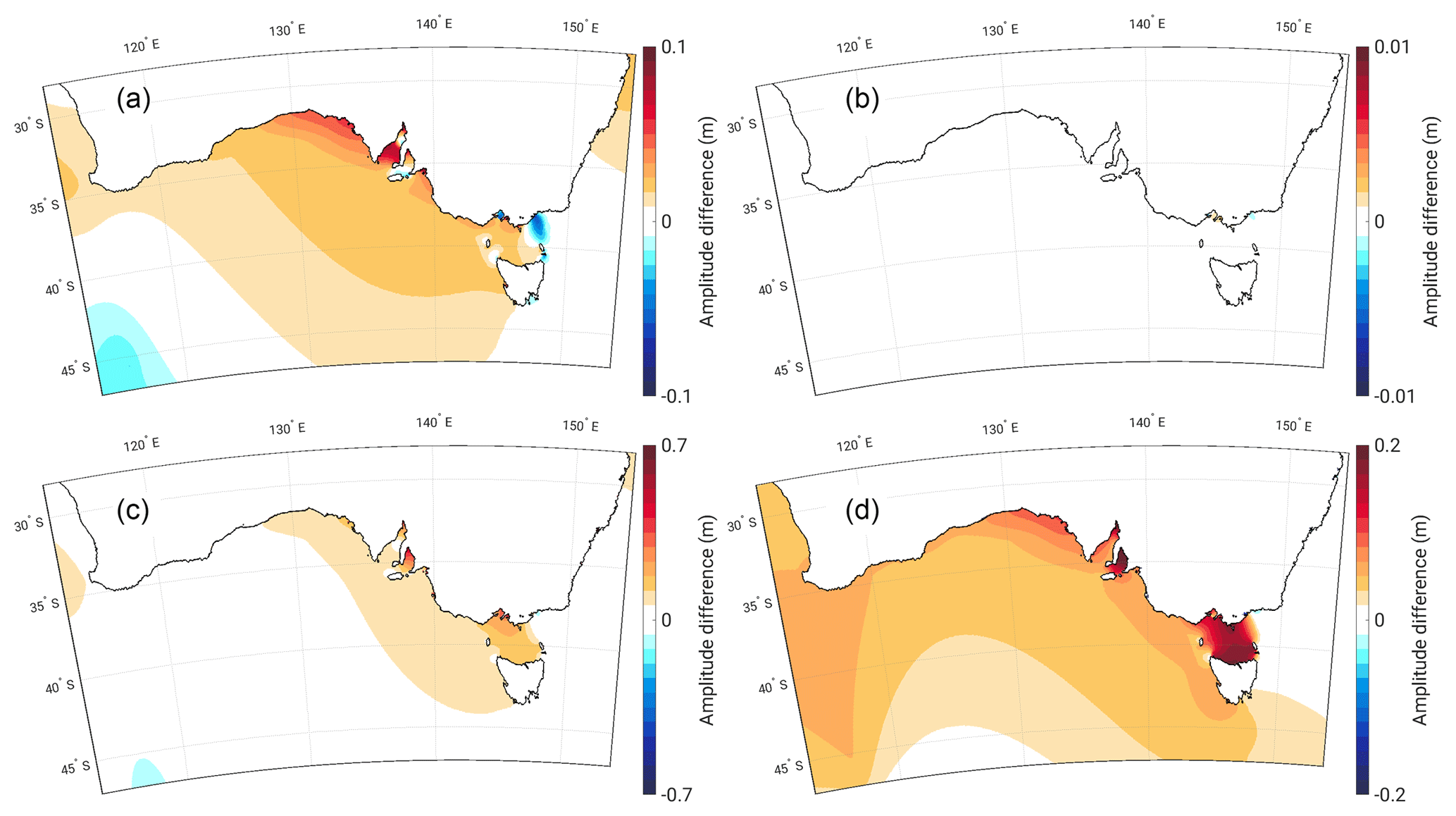
SLR brings some fairly significant changes to the M₂ tidal systems around Australia. Many of the regions which stand out as having high M₂ amplitude at present (see Fig. 1b) suffer a marked reduction in amplitude with increasing SLR (Fig. 5a and c). To the north-west of Australia, amplitudes decrease in regions centred around King Sound, around Joseph Bonaparte Gulf, within Van Diemen Gulf, and across the Timor Sea. The reduction in amplitude to the north-east of Van Diemen Gulf comes alongside the formation of a new amphidrome; the phase lines that run north-south in the Arafura Sea (Fig. 1b) move closer together before coalescing to form an amphidromic point. A further amphidromic point emerges in the south-east of the Gulf of Carpentaria, around the Wellesley Islands, when a virtual amphidromic point (an amphidrome over land) moves north to become real (an amphidrome over the ocean). Both these points form some time between 3 and 5 m SLR (not shown). The amphidrome that sits north of the Gulf of Carpentaria (Fig. 4a) moves northwards with SLR in both the FL and NFL scenarios, eventually becoming virtual at the higher SLR scenarios by moving over Yos Sudarso Island. This movement is therefore associated with the change in the propagation properties of the incoming tidal wave, rather than the inundation of Yos Sudarso Island which occurs at 5 m SLR and above.

The Torres Strait features a sharp divide between a large positive and small or weakly negative amplitude difference on its west and east sides, respectively. The strait is shallow and dotted with islands, restricting the flow of the tides. Absolute amplitudes on the east side are initially elevated compared to the west (Fig. 1b) but this difference is mitigated with increasing SLR, as the larger volume of the channel allows for enhanced tidal transport across the strait (Fig. 5a and c).

In the remaining part of the domain, the M₂ amplitudes around the coast of New Zealand and along the east coast of Australia, particularly between Hay Point and Gladstone (Fig. 1a, points 3 and 4), both increase with SLR. In the Bass Strait, shown in Fig. 6, the amplitude also increases along with SLR; however, there is a slight drop in amplitude at 1 m SLR at the eastern entrance of the strait and within Port Phillip Bay (the location of the Geelong and Williamstown tide gauges). These decreases quickly disappear at higher SLR. Along the south coast of Australia, the amplitudes also increase with SLR, but the simulated perturbations there are generally smaller in magnitude than in the north (see also Schindelegger et al., 2018). Increased tidal amplitudes at the head and mouth of Spencer Gulf (Fig. 6a) are associated with a slight weakening of a standing-wave-like pattern where M₂ amplitudes increase from the sea towards inland (Fig. 1b). However, this feature does not evolve proportionally with the imposed level of SLR (see Fig. 6c for the 7 m case). To the east, in Gulf St. Vincent, there is a similar, if stronger, standing-wave-like pattern (Fig. 1b). Here, the elevated amplitudes proximity to the coast increase in line with SLR (Fig. 6c). Moving further west along the south coast of Australia, the amphidromic point off the south-west coast moves southwards with increasing SLR (Fig. 4a and b), with a faster progression in the NFL than in the FL runs. Note that, almost universally across the domain, the amplitudes seen in the NFL runs are higher than those in the FL runs (Figs. 5d and 6d). It is clear that allowing flooding to occur suppresses the magnitude of any SLR effect upon tidal amplitude.

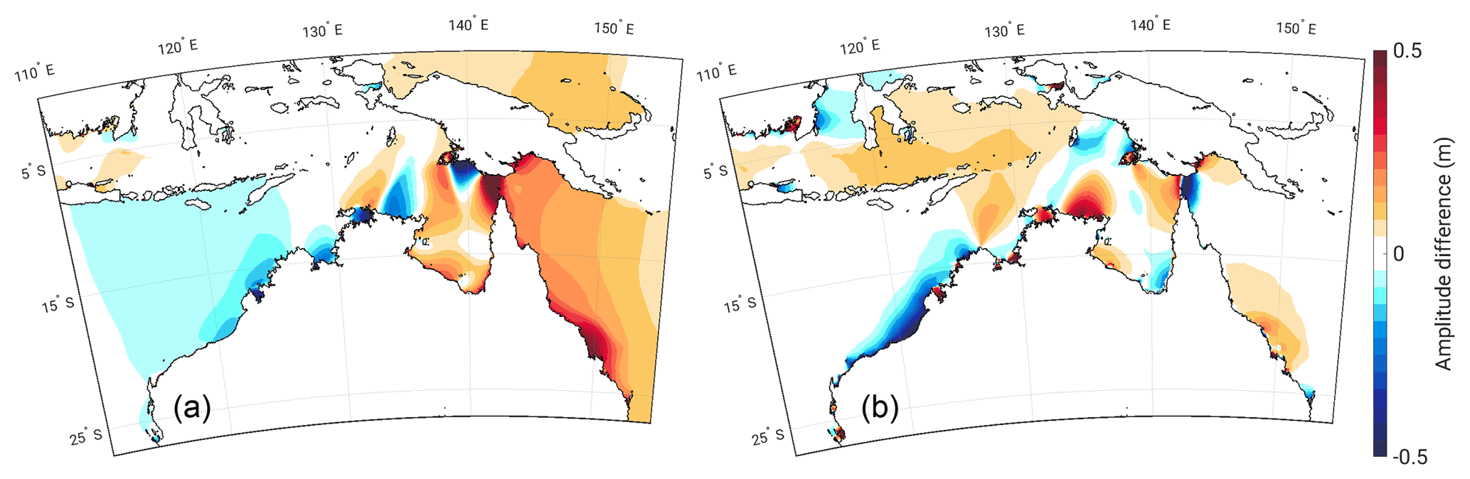
Figure 7The difference in M₂ amplitude (m) between the FL and control simulation (i.e. FL–control) for 7 m SLR using boundary conditions generated from a global 7 m SLR scenario (a) and using boundary conditions generated from TPXO8 (b).

Download

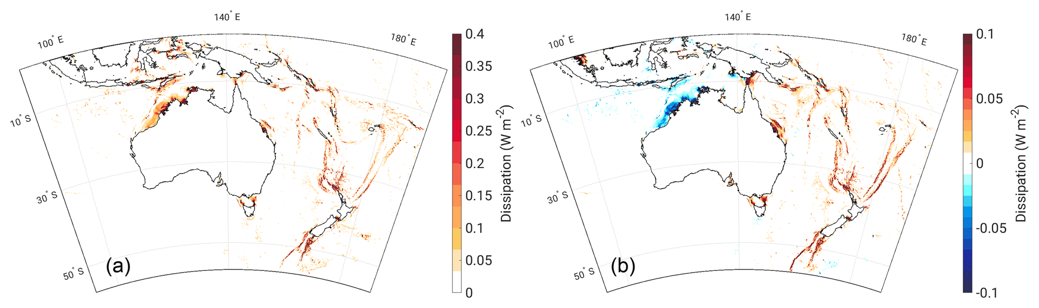
Figure 8The dissipation (W m⁻²) associated with the M₂ constituent across the entire model domain (a) and the difference in dissipation between the 7 m FL simulation and the control run (i.e. FL–control, b).

Download

Additionally, we have repeated our control and future simulations using boundary conditions taken from TPXO8, i.e. using present-day boundary conditions, instead of those from global SLR simulations. In these runs, the magnitude and spatial distribution of the amplitude changes are vastly different from the results presented above. Figure 7 demonstrates, and allows for a comparison of, the pattern of amplitude changes seen for M₂ north of Australia in these runs. Especially striking is the difference in magnitude of tidal amplitude increases along the east coast of Australia. Applying present-day boundary conditions leads to a very strong underestimation of the amplitude changes in this area (the differences exceed 40 cm in some locations). Similarly pronounced is the difference on the north-west coast where the run with present-day boundary conditions overestimates the amplitude decreases. In large parts of the Arafura Sea, the tidal amplitude responses are of opposite sign in response to the different boundary conditions. This is a key result and it highlights the importance of applying correct boundary conditions for regional simulations which take into account the far-field change occurring outside the model domain.

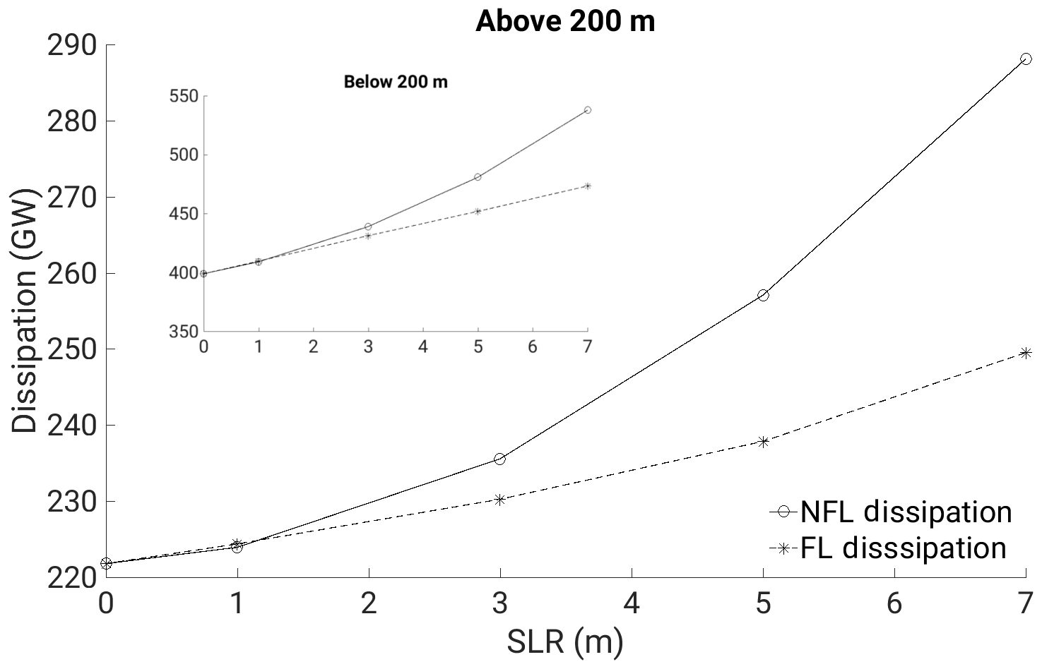
Figure 9The dissipation totals (GW) across the model domain above and below (inset) the depth of the 200 m isobath of the control bathymetry.

Download

Figure 10Same as Fig. 5 but for the K₁ constituent.

Download

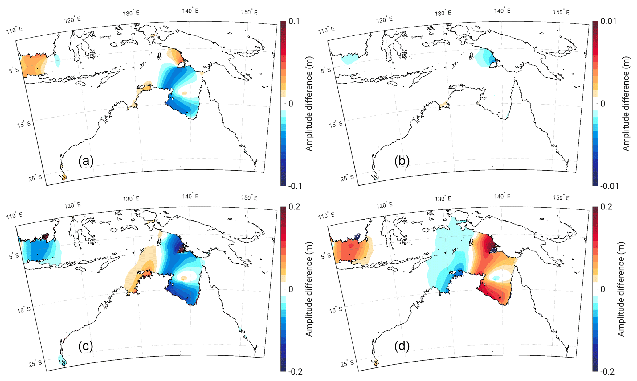
Figure 8a displays the dissipation associated with the M₂ tidal constituent for the control simulation. It is evident that a majority of the energy is lost at the coast and on the shelf, especially around sharp and shallow bathymetric features. There is a remarkable reduction in dissipation along the north-west coast of Australia with SLR, matching areas with a marked decrease in tidal amplitude (Fig. 8b). There are small pockets of dissipation increases in proximity to the coast in the north-west, associated with areas of enhanced flooding. Much of the dissipation increases within the domain come from the undersea ridges and trenches to the north and south of New Zealand, as well as the east side of the Torres Strait, the area between Hay Point and Gladstone on the east coast of Australia (at the southern extent of the Great Barrier Reef), and both ends of the Bass Strait. All of these areas are associated with an increase in M₂ amplitude with SLR.

The impact upon the total dissipation across the domain by allowing flooding is illustrated in Fig. 9. In both the NFL and FL runs, dissipation increases with SLR; the dissipation generated by areas with increased amplitudes outweighs the loss of dissipation in areas of decreased amplitude. With amplitudes in the NFL runs being much higher than in the FL runs, the corresponding dissipation is higher, and the gap in dissipation between the NFL and FL simulations widens with increasing SLR. At 12 m SLR, the NFL dissipation begins to plateau, whilst the FL dissipation continues to rise. Overall, dissipation on the shelf (nominally above the 200 m isobath, accounting for approximately 7 % of the water-covered area of the domain) amounts to about half of the energy dissipated in deeper water.

3.2 Effect of SLR on the K₁ tide

The changes to K₁ are relatively small in comparison to the changes seen for the semi-diurnal constituent. The main point of interest is the amphidromic system in the Gulf of Carpentaria. Figure 10 shows an initial negative amplitude response in the north and south of the Gulf, while there are slight increases in amplitude north of Yos Sudarso Island and in the Java Sea. The position of the amphidromic system is relatively stable with SLR, as evident from the constituent phase plots in Fig. 4c and d, and it is evident that K₁ suffers a decrease in amplitude around the Gulf of Carpentaria with SLR. Comparing Fig. 10c and d, a majority of the amplitude difference occurring in the FL scenario is negated when impermeable coastlines are implemented. The dissipation for which K₁ is responsible in the domain is approximately 7 times smaller than that of M₂ and therefore not discussed further.

3.3 Synthesis

One of the most striking characteristics of the response of the semi-diurnal constituents to SLR is the drop in amplitude along the north-west coast of Australia, an area where a large amount of dissipation occurs in the control. We associate this feature with the altered propagation properties of the incoming tidal wave, as the imposed sea-level change in our simulations represents a significant fraction of the average water depth across the shelf; for instance, the 7 m SLR scenario increases the depth of the Gulf of Carpentaria by ∼10 %. As the tidal system goes from hosting a single wave propagating across the Arafura Sea to something more complex with multiple amphidromes within the basin, the semi-diurnal resonant response on the shelf is interrupted. This dynamical change may explain the drop in amplitudes to the north-west of Australia.