the Creative Commons Attribution 4.0 License.
the Creative Commons Attribution 4.0 License.
 | 25 Nov 2019
Two typical merging events of oceanic mesoscale anticyclonic eddies
Zi-Fei Wang
Qiu-Yang Li
Hao Cheng
The long-term theoretical “energy paradox” of whether the final state of two merging anticyclones contains more energy than the initial state is studied by considering two typical merging events of ocean mesoscale eddies. The results demonstrate that the total mass (volume), total circulation (area integration of vorticity), and total angular momentum (AM) are conserved if the orbital AM relative to the center of mass is taken into account as the eddies rotate around the center of mass before merging. For subsurface merging, the mass trapped by the Taylor–Proudman effect above the subsurface eddies should also be included. Both conservation laws of circulation and orbital AM have been overlooked in previous theoretical studies. As a result of fusion during merging, the total eddy kinetic energy decreases slightly. In contrast, the total eddy potential energy (EPE) increases after merging. The increase in EPE is mostly supported by the loss of gravitational potential energy (PE) via eddy sinking below the original level prior to merging. This implies that the merging of eddies requires background gravitational PE to be converted to EPE. In contrast, the vorticity and enstrophy consequently decrease after merging. Thus, the eddy merging effect behaves as a “large-scale energy pump” in an inverse energy cascade. It is noted that eddy conservation and conversion laws depend on the laws of physical dynamics, even if additional degrees of freedom can be provided in a mathematical model.
- Article
(6550 KB) - Companion paper
- BibTeX
- EndNote


Mesoscale eddies, i.e., coherent vortices with a rotational core, usually have a long life cycle of weeks or months and transport heat, salt, and other passive tracers over long distances (Chelton et al., 2011; Dong et al., 2014; McGillicuddy, 2011; Zhang et al., 2014; Bosse et al., 2019) by trapping tracers with the water (Xu et al., 2014; Torres et al., 2018). During the lifetime of an eddy, complex dynamic processes, such as merging and splitting, which are associated with eddy genesis and termination, often occur. This in turn modulates the eddy's life cycle and transports. In addition, there are incoherent eddies, which typically do not have a core or a well-defined eddy radius. These incoherent eddies are also important because they contain most of the eddy kinetic energy (EKE) in the ocean (Torres et al., 2018) and are responsible for most of the eddy transport of tracers (Su et al., 2018; Zhang et al., 2019).
There is a long-term unresolved “paradox” pertaining to the merging of two like-signed oceanic mesoscale eddies, i.e., whether the merged eddy has more or less energy than the sum of the two original eddies. This paradox first emerged from a theoretical study on the merging of two anticyclonic, zero-potential-vorticity plane eddies by Gill and Griffiths (Nof and Simon, 1987; Cushman-Roisin, 1989; Lumpkin et al., 2000). According to the theory, if mass and potential vorticity are conserved by two anticyclones, the final state should contain more energy than the initial state, which implies that an additional amount of energy must be supplied to complete the process. This study seemed to open a “Pandora's box”, as subsequent studies were in contradiction about which eddy properties (mass, potential vorticity, energy, angular momentum) should be conserved after merging. The conservation of mass is a generally accepted assumption and has been validated in experiments (Nof and Simon, 1987). However, there are still some merger scenarios in which mass is not conserved (Cushman-Roisin, 1989; Lumpkin et al., 2000). Similarly, the conservation of potential vorticity (PV) (Gill and Griffiths, unpublished; Cushman-Roisin, 1989; Nof, 1990) has been abandoned in some studies (Griffiths and Hopfinger, 1987; Nof and Simon, 1987; Nof, 1988; Lumpkin et al., 2000). In contrast, the previously overlooked conservation of angular momentum (AM) (Cushman-Roisin, 1989) has become generally accepted in various models (Nof, 1990; Pavia and Cushman-Roisin, 1990; Lumpkin et al., 2000). Consequently, in theoretical scenarios of merging, the merged eddy might have less (Lumpkin et al., 2000), the same (Nof and Simon, 1987; Pavia and Cushman-Roisin, 1990; Lumpkin et al., 2000), or more energy (Griffiths and Hopfinger, 1987) than before merging, depending on the assumptions. Because these eddy models have only two parameters (amplitude and radius), there is the dilemma of the parameters being less numerous than the conservation laws (e.g., mass, vorticity, momentum, energy) (Pavia and Cushman-Roisin, 1990; Lumpkin et al., 2000). This leads again to the question of which conservation laws should be applied to eddy merger (Lumpkin et al., 2000). One possible way to solve this dilemma is to use a complex eddy model with more parameters, with which more conservation laws might be held simultaneously.
In addition, an effective way to dispel this “paradox” in eddy merger scenarios is to use oceanic observations to examine the above assumptions. However, this has seldom been studied because the field observations by research cruises and floats can hardly capture eddy merger events, except in only a few cases (Cresswell, 1982; Sangra et al., 2005; Raj et al., 2016). On the other hand, satellite observations provide a different way of observing eddy motions. Based on sea level anomaly (SLA) data, the Genealogical Evolution Model (GEM), an efficient logical model, was developed to track the dynamic evolution (merging and splitting) of eddies (Li et al., 2014, 2016).
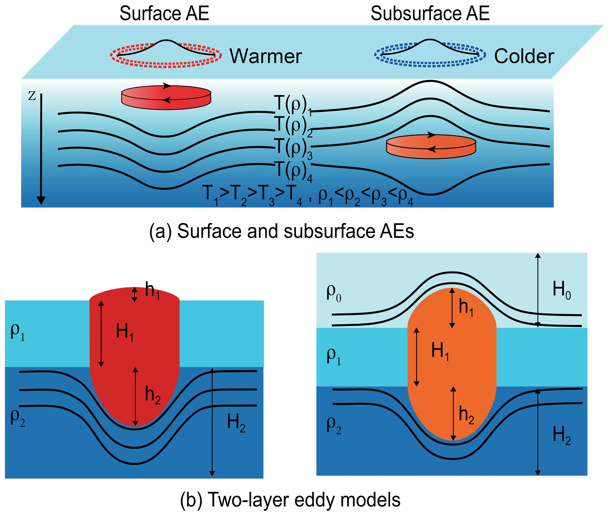
Figure 1(a) Surface and subsurface anticyclonic eddies (AEs) and (b) two-layer eddy models used in the present study.
The motivation of this study was to test the conservation laws without any prior assumptions of conservation by calculating the eddy properties. To this end, we firstly chose two typical merger events by using the GEM. Next, the eddies were distinguished as surface or subsurface eddies (Fig. 1a) according to sea surface temperature (SST) data (Assassi et al., 2016). Secondly, we used a vertical two-layer model (Fig. 1b) (Lumpkin et al., 2000) and a Gaussian model for horizontal shape according to observations (Wang et al., 2015; Yi et al., 2015). There were many more eddy parameters than potential conservation laws, which avoided the aforementioned dilemma. Thirdly, we estimated pre- and post-merging eddy parameters (Fig. 1a, b) with a nonlinear optimal fitting approach (Wang et al., 2015). Finally, we calculated the eddy properties to determine what occurred after the two typical eddy mergers.
The paper is structured as follows. A brief description of the data, eddy identification, eddy parameters, and eddy properties is presented in Sect. 2. In Sect. 3, the merging processes of surface anticyclonic eddies (AEs) and subsurface AEs are both described, and then the conservation and conversion laws are tested by using the eddy properties. The sensitivity of the result to the parameters is discussed in Sect. 4. Finally, the conclusions are presented in Sect. 5.
2.1 Data
The SLA data used here were from the merged and gridded satellite product of MSLA (Maps of SLA), which is produced and distributed by AVISO (Archiving, Validation, and Interpretation of Satellite Oceanographic data)(https://www.aviso.altimetry.fr/, last access: 18 November 2019) based on TOPEX/Poseidon, Jason-1, ERS-1, and ERS-2 data (Ducet et al., 2000). Currently, the products are available on a daily scale with resolution for the global ocean as DUACS DT14 (Pujol et al., 2016). It is worth pointing out that such resolution applies only to the data resolution, not the physical signal resolution, due to AVISO's low resolution of 100–200 km (Ducet et al., 2000; Chelton et al., 2011; Amores et al., 2018; Ballarotta et al., 2019).
The SST data were produced by the Operational Sea Surface Temperature and Sea Ice Analysis (OSTIA) system (Donlon et al., 2012) and downloaded at the Asia-Pacific Data-Research Center (APDRC http://apdrc.soest.hawaii.edu/data/, last access: 18 November 2019). The analysis of SST data has global coverage with a spatial resolution of and a temporal resolution of 1 d. The ocean vertical density profile data were from the NCEP (National Centers for Environmental Prediction) Global Ocean Data Assimilation System (GODAS) (Behringer et al., 2004) and were downloaded from NOAA (National Oceanic and Atmospheric Administration) (https://www.esrl.noaa.gov/psd/data/gridded/data.godas.html, last access: 18 November 2019).
Eddy merger events were tracked using the GEM (Li and Sun, 2015; Li et al., 2016), which is an efficient logical model for tracking the dynamic evolution of mesoscale eddies (merging and splitting) from satellite SLA data.
2.2 Identification of surface and subsurface anticyclonic eddies
Surface eddies are distinguished from subsurface eddies by whether their core is in the surface layer or located inside the water column (Fig. 1a). Consequently, the surface AEs have positive SST anomalies (SSTAs) and the subsurface AEs have negative SSTAs (Assassi et al., 2016). Here, we used the method proposed by Assassi et al. (2016) to identify surface AEs (SSTA > 0) and subsurface AEs (SSTA < 0). The SSTA was obtained by removing the background SST, which is the weighted average of the SST within the box, as used previously (Assassi et al., 2016).
2.3 Eddy parameters
In this study, we used a Gaussian model for SLAs, which is the most typical model for ocean mesoscale eddies (Wang et al., 2015; Yang et al., 2019), to obtain the eddy properties. The SLA field h(x,y) with several adjacent eddies before merging can be expressed as (Yi et al., 2015; Chen et al., 2019)
where x, y are the zonal and meridional coordinates, respectively; x0, y0 is the position of the eddy center; Lx and Ly correspond to the longitude and latitude radii, respectively; and A denotes the eddy amplitude. The eddy parameters (A, Lx, and Ly) are obtained by using nonlinear fitting (Wang et al., 2015). The eddy size, i.e., eddy area S=πLxLy, is calculated by integrating an ellipse. It is useful to point out that eddy area is an extensive quantity; this is the reason why the eddy area is the intrinsic parameter in estimating eddy viscosity (Li et al., 2018). Next, the velocity (u, v) and vorticity (ξ) of the eddy field are calculated by geostrophic approximation (if the x and y axis origins are at the eddy center).
The parameter b represents the vertical eddy shift, which is critical for properly composing and fitting the eddy parameters (Wang et al., 2015). In addition, in this study, we point out for the first time that it is associated with the potential energy (PE) conversion balance.
For a two-layer model, as shown in Fig. 1b, the upper (lower) layer has a thickness of H1 (H2) and a density of ρ1 (ρ2). The surface AE consists of three parts – the upper surface h1=A, the lower surface , and the eddy body of height H1. Typically, we have . If both h1 and h2 are very small and can be ignored, the model becomes a one-layer model of a cylinder (Sangra et al., 2005) or a plane model, as used in many previous theoretical models. On the other hand, if H1 is too small to be ignored, it becomes a lens model (e.g., Lumpkin et al., 2000). For subsurface AEs, there is an additional surface layer of thickness H0 and density ρ0 over the eddy (Fig. 1b). The upper surface and the lower surface satisfy . In the present study, both H0 and H1 were chosen to be 200 m, partly according to some recent observations (Zhang et al., 2015; Bashmachnikov, 2017; Li et al., 2017; Wang, 2017; Mason et al., 2019). The sensitivity of the result to choice of depth is discussed in Sect. 4.
2.4 Eddy properties
The eddy properties are calculated by integration of the proper parameters within an eddy. The originally identified boundary of an eddy may lead to an unexpected sharp decrease in eddy properties before merger (e.g., Laxenaire et al., 2018; Cui et al., 2019). This is mainly due to the previous eddy detection methods lacking a proper segmentation algorithm, which was illustrated in Li and Sun (2015). In this study, the integration area is an ellipse with a major axis and a minor axis of 2Lx and 2Ly, respectively. As the density varies little from surface to deep sea, the anticyclone mass is calculated by numerical integration of volume:
where H1 is the depth of the vortex body layer and h1 and h2 are the upper and lower interface anomalies, respectively, as shown in Fig. 1b. The relative eddy circulation Γ is calculated by surface integration of PV (Gill, 1982, p. 192),
or volume integration of the PV anomaly (Gill, 1982, p. 192):
where f is the Coriolis parameter. The relative PV anomaly mean is the area average of circulation Γ. The relative AM is calculated by integration of torque, where the x and y axis origins are at the eddy center:
The EKE per mass is calculated by integration as follows:
The eddy potential energy (EPE) consists of the effective PE of the upper interface and the lower interface, as H1 does not change during the merging process (e.g., Lumpkin et al., 2000):
where and are the reduced gravity. The eddy enstrophy is calculated by integration:
The eddy gravitational PE referring to background sea level with the eddy shift parameter b is calculated as follows:
2.5 Error estimation
Since the above eddy properties and parameters are calculated from the SLA field, we need to estimate the errors of the values from the calculation. We first estimate the errors of eddy parameters (e.g., A, Lx, and Ly) obtained by nonlinear fitting (https://ww2.mathworks.cn/help/curvefit/confidence-and-prediction-bounds.html, last access: 18 November 2019). This is simple, because the outputs of the fitting algorithm (Wang et al., 2015) have already included the standard deviation (e.g., δA,δb and δS) of each parameter and the coefficient of determination (R2). Typically, the standard deviations are 2 %–8 % of eddy parameters, and the fitting performance R2 is 0.87 to 0.98 in this study.
Secondly, we estimate the standard deviations of eddy properties. Since we have used numerical integration of eddy parameters to obtain eddy properties, there are no simple and explicit relations between eddy properties and eddy parameters. The exact standard deviations of eddy properties can hardly be obtained in this way. Here we approximately estimate the standard deviations of eddy properties by assuming that the eddy is a circle with the same area S of the original ellipse. Then the eddy properties can be expressed as functions of eddy parameters (e.g., A and S) after integration. The standard deviations of eddy properties can now be estimated with standard deviations of eddy parameters. For example, the eddy enstrophy in Eq. (9) is , where c is the integration constant. Then the standard deviations of eddy enstrophy are . We use these standard deviations to draw error bars in figures.
3.1 Merging of surface AEs
The merging event consists of two AEs (AE1 and AE2) south of the Kuroshio extension within 17 to 22∘ N and 180 to 174∘ W from 19 May to 10 June 2013 (Fig. 2). Before the merging, AE1 was located at approximately 19∘ N and 178∘ W and AE2 was located to its northeast (Fig. 2a). As both eddies had positive SSTAs, they were surface AEs, as discussed in Sect. 2. Both eddies then moved westward from 178 to 179∘ W (Fig. 2d). During this time, AE1 and AE2 co-rotated anticyclonically. This co-rotation was also observed by Li et al. (2016). Next, AE1 and AE2 gradually merged into a larger AE on 1 June (Fig. 2c). In this case, the upper (lower) layer, ranging from 0 to 200 m (200 to 1000 m) depth, had a mean density of 1024.2 (1029.4) kg m−3, according to the GODAS data for this region. The height of the eddy body H1 was 200 m, and the lower surface height h2 (27.3 m) was approximately 195 times that of the eddy amplitude h1 (0.14 m).
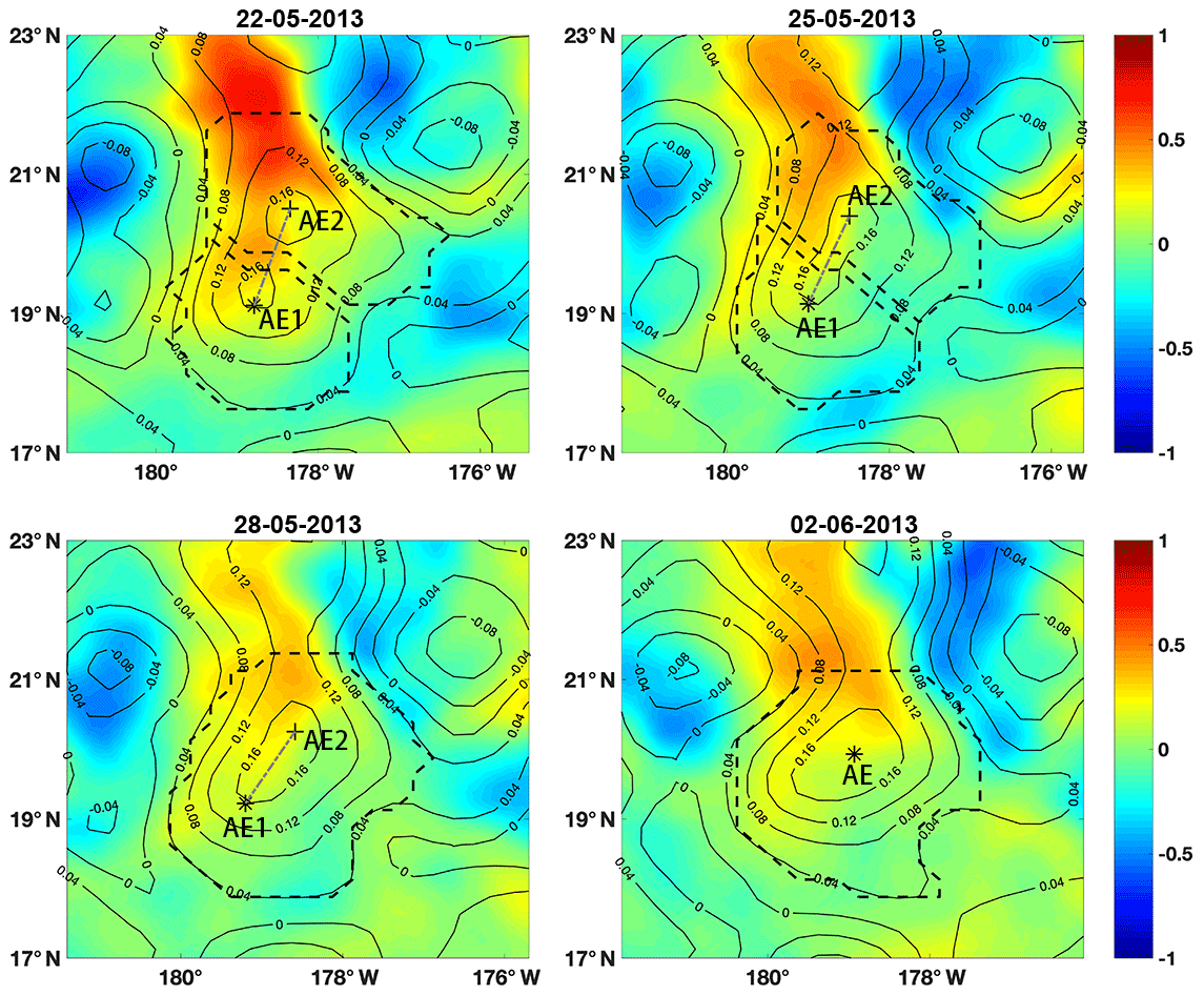
Figure 2Merging event of surface anticyclonic eddies. The colors and contours represent SST and SLA values, respectively. The eddy boundaries are labeled with dashed curves. The cross and asterisk represent eddy centers identified by the fitting method. The dashed line connecting eddy centers rotates anticyclonically during the merging event.
To illustrate clearly how the eddies changed during the merging process, we first calculated the parameters of both eddies. It is obvious that both eddies had positive SSTAs and that the merged AE also had positive SSTAs (Fig. 3a). They all were surface AEs. The fitted eddy parameters are shown in Fig. 3a. The first fitted parameter is the vertical shift b, representing the background SLA. In this case, b was very small, and it decreased a small amount from approximately 0.045 m before the merging to 0.038 m after the merging. The second parameter is the amplitude of the eddy. Before merging, the amplitude of AE2 increased gradually from 0.12 to 0.14 m and, notably, the amplitude of AE1 decreased gradually from 0.12 to 0.08 m. After merging, the amplitude of the merged eddy increased continually from 0.16 to 0.17 m. In contrast, the area of each eddy seldom changed before the merging. AE2 had a large area of 1.7×10⁴ km2, and AE1 had a smaller area of 0.9×10⁴ km2.
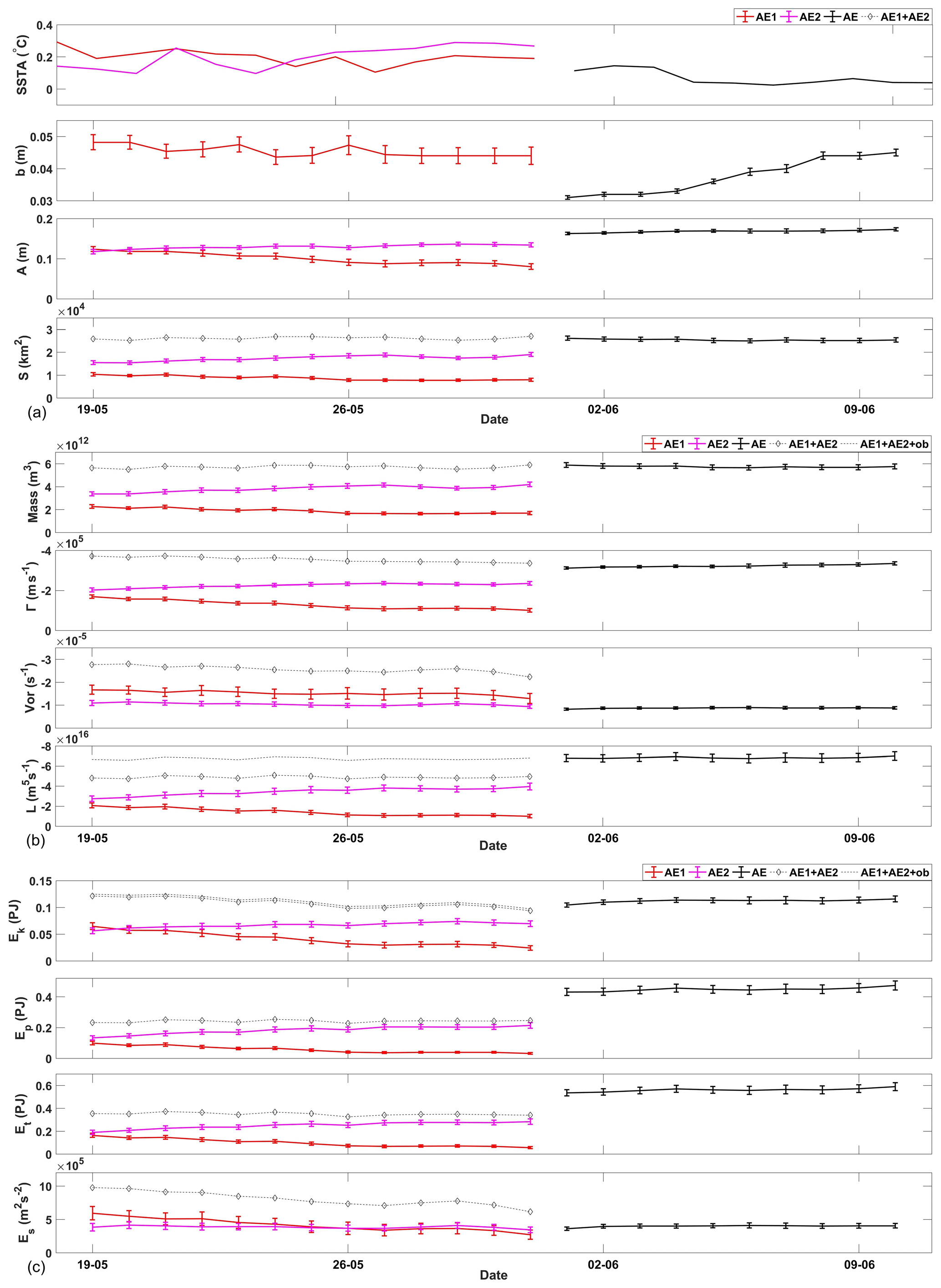
Figure 3The parameters in the merging event of the surface mesoscale eddies, where “AE1”, “AE2”, and “AE” represent the eddies, respectively, and “ob” represents the orbital AM associated with co-rotation. The error bars indicate the standard deviation of the value. (a) SSTA, background parameter, eddy amplitude, and eddy area; (b) mass, circulation, vorticity, and angular momentum; and (c) EKE, EPE, total mechanical energy, and enstrophy.
Next, we calculated the eddy properties using the above parameters. The mass (volume) of the eddies experienced changes similar to those of the eddy area (Fig. 3b). This occurred because H1 dominates the whole depth as . The relative PV was averaged within each eddy. As shown in Fig. 3b, the vorticity of AE2 varied by a very small amount and the vorticity of AE1 decreased gradually before merging. It is noted that the vorticity of AE2 was significantly smaller, although it had a larger amplitude, which was obtained from the SLA field according to Eq. (1). This is because vorticity is not only proportional to eddy amplitude, but is also inversely proportional to eddy area. After the merging, the vorticity of the merged eddy became very small, significantly smaller than that of AE2. The calculated circulation and AM of the eddy are shown in Fig. 3b. The results are similar to those for the amplitude, i.e., a larger amplitude with larger circulation and larger AM.
Finally, we calculated the energies of the eddies. Both the EKE and EPE had similar variations before the merging. However, they were quite different after the merging: EKE decreased but EPE increased. This point is addressed in detail in the following subsection.
3.2 Merging of subsurface AEs
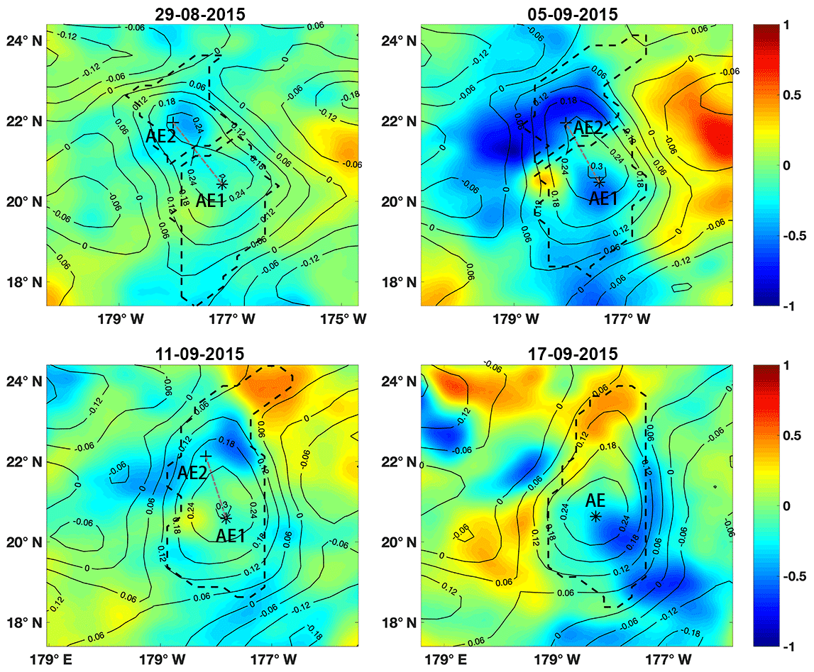
The second typical horizontal merging process was between two subsurface anticyclones. It occurred in the period from 29 August to 22 September 2015, in the region between 18 and 23∘ north latitude and 179∘ east longitude and 175∘ west longitude, roughly to the west of the surface vortex merging event described in the previous section. In this case, three layers were divided as 0–200, 200–400, and 400–1000 m, respectively. The mean densities of the layers were 1024.2, 1028.0, and 1030.8 kg m−3, respectively, according to the GODAS data for the regions. The height of the eddy body H1 was 200 m, and the upper (lower) surface height h1 (h2) was 104 m (98.4 m), approximately 348 (328) times the eddy amplitude.
At the beginning of the merging, anticyclone AE1 was located at approximately 20∘ N latitude and 177∘ W longitude, and AE2 was northwestward alongside AE1. Then, AE1 and AE2 approached each other with a clockwise rotation and eventually merged into AE on 13 September. Similarly, Fig. 4 shows a series of snapshots of this subsurface merging event. It can be seen that there is a clear cold core filled by a negative SSTA in each of AE1, AE2, and AE at the beginning (top two subfigures) and ending (bottom two subfigures) stages of the process, representing a distinct anticyclonic surface vortex signal. We also noticed that during the middle of the process, on 5 September, the cold core structures were interrupted by positive SSTA areas, a small area between AE1 and AE2, and a large area, with a diameter of approximately 0.5∘, west of AE1, until the two anticyclones merged. On 14 September, the cold core structure of the merged vortex AE was clear again. This may have been caused by the intense mixing effect in the eddy–eddy interactions, especially when the two like-sign vortices came close to each other. However, the type of vortex should be determined by the relatively stable continuous stage over a period of time before and after the merging, so this sudden change would not affect the identification of subsurface AE in this case.
To illustrate clearly what occurred for the eddies during the merging process, we first calculated both eddy parameters. It is obvious that the surface eddy had a positive SSTA, but the subsurface eddy had a negative SSTA. The merged AE had a positive SSTA (Fig. 5a), i.e., the surface eddy covered the subsurface eddy. The fitted eddy parameters are shown in Fig. 5a. The first fitted parameter is the vertical shift b, representing the background SLA. In this case, b was very small and decreased by a small amount, from approximately 0.020 m before merging to 0.001 m after merging. The second parameter is the amplitude of the eddy. Before merging, the amplitude of AE1 increased gradually from 0.28 to 0.30 m, while the amplitude of AE2 decreased notably from 0.22 to 0.14 m. After merging, the merged eddy had an amplitude of 0.30 m, similar to that of AE1. In contrast, the areas of the two eddies seldom changed before merging. AE1 had a large area of 2.39×10⁴ km2, while AE2 had a smaller area of 1.18×10⁴ km2.
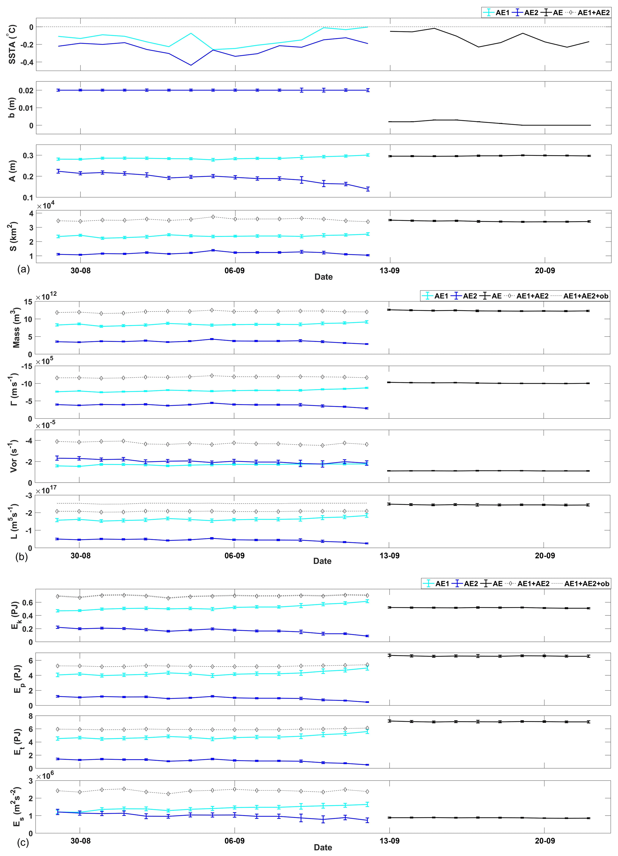
Next, we calculated the eddy properties using the above parameters. The mass (volume) of the eddies experienced changes that were similar to those of the eddy area (Fig. 5b). This occurred because H1 dominates the whole depth, although h1 is on the same order as h2. The relative PV was averaged within each eddy. As shown in Fig. 5b, the vorticity of AE1 varied by a very small amount and the vorticity of AE2 decreased gradually before merging. It is noted that the vorticity of AE2 was significantly smaller, although it had a larger amplitude. This is because vorticity is not only proportional to amplitude but also inversely proportional to area. After merging, the vorticity of the merged eddy became very small, significantly smaller than that of AE2. Next, the circulation and AM of the eddy were calculated, as shown in Fig. 5b. The results are similar to those for the amplitude – larger amplitude with larger circulation and larger AM.
Finally, we calculated the energies of the eddies. Both the EKE and EPE had similar variations before merging. However, they were quite different after merging: EKE decreased but EPE increased. This is addressed in detail in the following subsection.
3.3 Conservation and conversion laws
First, we examined whether the total volume (mass) of the eddies was conserved. In the first case, the total volumes pre- and post-merging were and m3, respectively, where the plus/minus amounts are standard deviations of the values. In the second case, the total volumes pre- and post-merging were and m3, respectively. As shown in Figs. 3a and 5a, the total volume seldom changed in both cases. It is obvious that the merging events obeyed the law of conservation of mass.
The second conservation law is conservation of total circulation. In both cases, the total circulation of the eddies seldom changed (Figs. 3b and 5b). If circulation is conserved, the flow is referred to as circulation-preserving flow (Wu et al., 2007). Circulation-preserving flow has minimum total enstrophy and minimum dissipation according to the Helmholtz–Rayleigh minimum dissipation theorem. The conservation of total circulation provides a method for calculating the vorticity of the merged eddy, because single-eddy PV is not conserved in eddy merging events.
The third conservation law is for total AM. In the first case, the total AM before merging was m5 s−1, while the merged AM was m5 s−1. The merged AM is significantly larger than the pre-merging value. Thus, the merged eddy should have some additional sources of AM, which were ignored in previous studies. One possible source of the missing AM is orbital AM; both eddies co-rotated around the center of mass with an angular speed ω of d−1, as mentioned previously. This co-rotation provided additional AM of approximately 1.841×10¹⁶ m5 s−1, or 38 % of the AM in both eddies. After accounting for the orbital AM contributed to the system, the total AM is approximately 6.718×10¹⁶ m5 s−1, which is almost the same as that after merging. Thus, by accounting for the orbital AM, the total AM is conserved. In the second case, the total AM before and after merging was and m5 s−1, respectively. The eddies co-rotated around the center of mass with an angular speed ω of d−1, which provided an orbital AM of 0.343×10¹⁷ m5 s−1. In addition, if the water above the two subsurface AEs was involved in such orbital AM due to the Taylor–Proudman effect, there should be an additional amount of 0.110×10¹⁷ m5 s−1. According to the Taylor–Proudman theorem, the water was attached to the moving eddies under the geostrophic condition. Thus, the total orbital AM is 0.453×10¹⁷ m5 s−1, approximately 22 % of the AM in both eddies. After accounting for the orbital AM to the system, the total AM is approximately 2.523×10¹⁷ m5 s−1, which is almost the same as the value after merging. In both cases, the orbital AM is non-negligible.
The law of conservation of total AM was used in previous theoretical models, but without consideration of orbital AM. These calculations of total AM assumed that eddies were immersed in a quiescent fluid (Pavia and Cushman-Roisin, 1990; Lumpkin et al., 2000), i.e., that eddies were motionless before merging. However, this is not true because two approaching eddies would rotate around the center of mass according to fluid dynamics. This rotation was also noted in previously observed eddy merging events (Schultz Tokos et al., 1994; Li et al., 2016). Because the previous theoretical studies overlooked orbital AM, the calculations led to an incorrect AM balance between pre- and post-merging stages.
Although the laws of conservation of total circulation and conservation of total AM are associated with rotation of water, they are somewhat different from the above analysis. The law of conservation of total circulation is only associated with eddy circulation, which is easy to use in applications. However, the conservation of total AM should consider both eddy circulation, referring to the center of each eddy, and orbital AM, referring to the whole system, which is difficult to calculate in complex environments.
In both cases, the total EKE decreased by a small amount after merging due to fusion. In the first case, the total EKE decreased from an initial range of 0.121 to 0.094 PJ (0.021 to 0.016 m2 s−2) before merging and then increased from 0.105 to 0.116 PJ (0.017 to 0.020 m2 s−2) after merging. The co-rotation also contributed approximately 3.4 TJ ( m2 s−2), a negligible value for total EKE. In the second case, the total EKE decreased from an initial range of 0.692±0.01 to 0.516±0.004 PJ (0.056 to 0.041 m2 s−2) after merging. The co-rotation also contributed a negligible value of 0.0068 PJ ( m2 s−2) in total EKE. Such a decrease in total EKE was noted in a previous study (Nof, 1990), in which EKE was the only component of energy in the theoretical one-layer model.
By contrast, the total PE increased significantly after merging. In the first case, the total PE increased by approximately 0.207 PJ (0.035 m2 s−2), from an initial range of 0.241±0.008 to 0.448±0.01 PJ (0.041 to 0.076 m2 s−2). In the second case, the total PE increased by approximately 1.343 (0.096 m2 s−2), from an initial range of 5.229±0.07 to 6.572±0.04 PJ (0.423 to 0.519 m2 s−2). The large increase in PE cannot be explained by the loss of EKE because eddy PE is, in general, an order of magnitude larger than the EKE (Su and Ingersoll, 2016). Thus, additional PE from the background environment contributed to the EPE, supporting the merging events, and the total mechanical energy increased after merging. Both the summer and autumn seasons are favorable for this merging condition in oceans of the Northern Hemisphere, which consequently leads to fewer eddies in these seasons, as noted before. This leads to the question of where the huge additional PE came from.
To find the source of the EPE increase, we calculated the change in eddy gravitational PE, referring to the background sea level, with eddy shift parameter b, according to Eq. (10). In the first case (Fig. 3a), b decreased from 0.045 to 0.038 m after merging. This slight vertical sink of the eddy released approximately 0.401 PJ (0.069 m2 s−2) of gravitational PE, 51.6 % of which accounts for the EPE increase. In the second case (Fig. 5a), b decreased from 0.02 to 0.001 m after merging. The vertical sink of the eddies released approximately 2.29 PJ (0.185 m2 s−2) of gravitational PE, 58.6 % of which accounts for the EPE increase. Thus, the vertical sink of the eddies released gravitational PE that supported the EPE increase. In addition, it can be deduced that the sink occurred at the level below the eddies; otherwise, it could not provide sufficient gravitational PE. For example, if only the surface water sank to the level of b, the released gravitational PE would be much less than the aforementioned values. This implies that such gravitational PE may be released from the ocean interior, deep below the upper ocean layer. It is also deduced that subsurface eddies might have a larger PV than surface eddies. A deeper eddy may have larger gravitational PE. Thus, merged eddies have additional PE conversion from the background gravitational PE below the eddies, which has not been noted previously.
Similar to the results of some previous theoretical studies (Griffiths and Hopfinger, 1987; Pavia and Cushman-Roisin, 1990), the total mechanical energy increased after merging, and vice versa, in the present work. On the other hand, eddies will merge if external energy is input into them. An underrated paper illustrates such a phenomenon (Carnevale and Vallis, 1990). Compared with these studies, our new findings are that the eddy PE dominates the increase in total mechanical energy (i.e., the sum of EKE and EPE) and that the EPE increase is converted from the eddy body sink.
Although the total circulation was conserved, the mean PV decreased after the merging in both cases due to the increase in eddy area. PV conservation has been generally assumed in theoretical models (Cushman-Roisin, 1989; Pavia and Cushman-Roisin, 1990; Nof, 1990), although others have stressed that the PV of eddies alternates during the interaction of merging (Gill and Hopfinger, 1987; Nof and Simon, 1987). Here, we point out that the total circulation conservation other than the individual eddy PV conservation becomes a constraint for eddy merging.
The eddy enstrophy decreased after merging, becoming even smaller than the mean enstrophy of the eddies (Figs. 3c and 5c). Because the EKE dissipation rate is proportional to the eddy enstrophy (Li et al., 2018), the merged eddies have a smaller dissipation rate, which might support a potentially longer eddy lifetime.
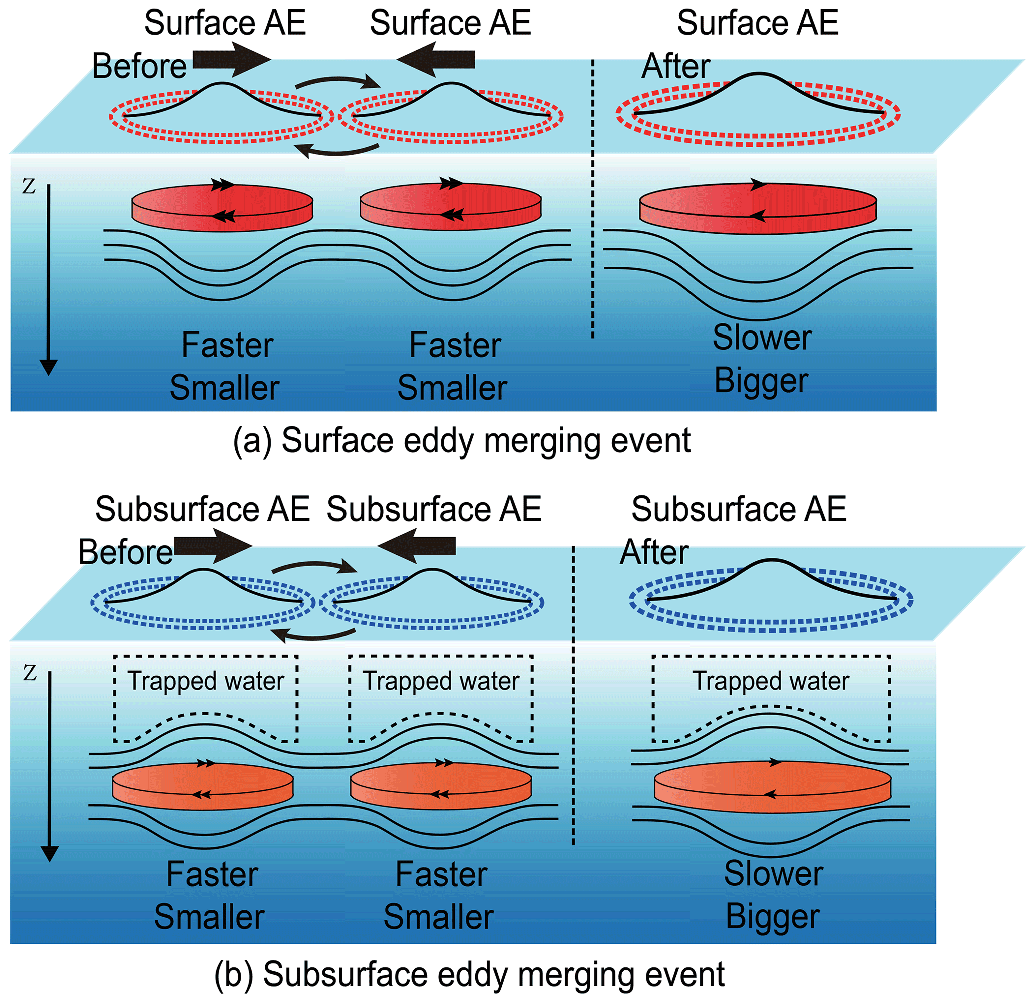
Table 1Observed physical quantity changes after merging events and conjectured changes after splitting events.
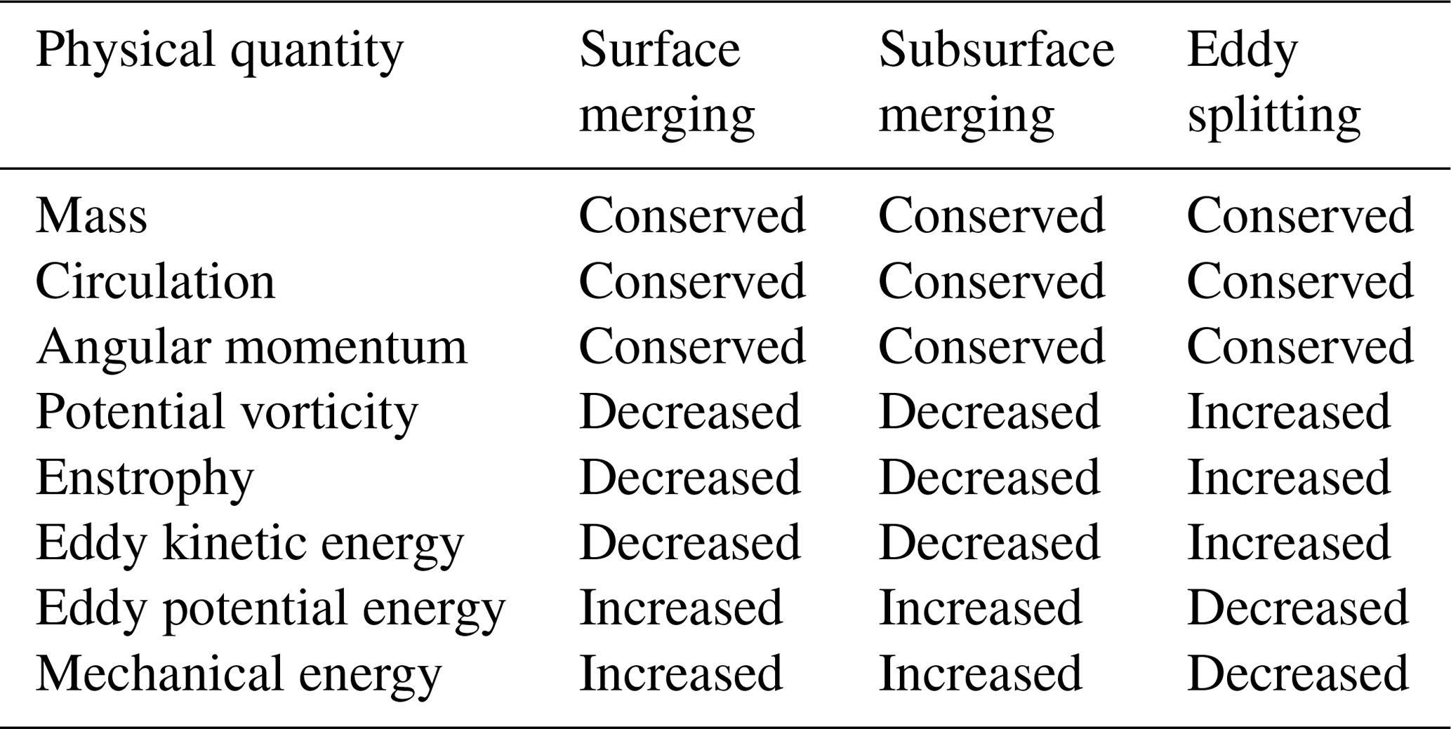
The observed changes in physical quantities after the merger events are listed in Table 1. Only three physical quantities (mass, circulation, and angular momentum) are conserved; the others have notable changes. The eddy merger is represented simply in the schematic diagram below (Fig. 6). Two faster and smaller eddies approach each other before the merger. During this time, they co-rotate anticyclonically with the water trapped by the eddies. Then, the two eddies coalesce into a slower and larger eddy. Both the surface eddy merger and the subsurface eddy merger satisfy the same conservation and conversion laws, as addressed above. The only annotation is that the water above the two subsurface AEs should be involved due to the Taylor–Proudman effect.
Eddy merging events could play a role in inverse energy cascades from small scale to large scale in two ways. On the one hand, merging functions similarly to a pump EKE and EPE from small-scale eddies to large-scale eddies. On the other hand, the EKE of large-scale eddies has a lower dissipation rate and a longer residence time. Thus, eddy merging functions like a “large-scale energy pump” in the inverse energy cascades (Qiu et al., 2017; Klein et al., 2019).
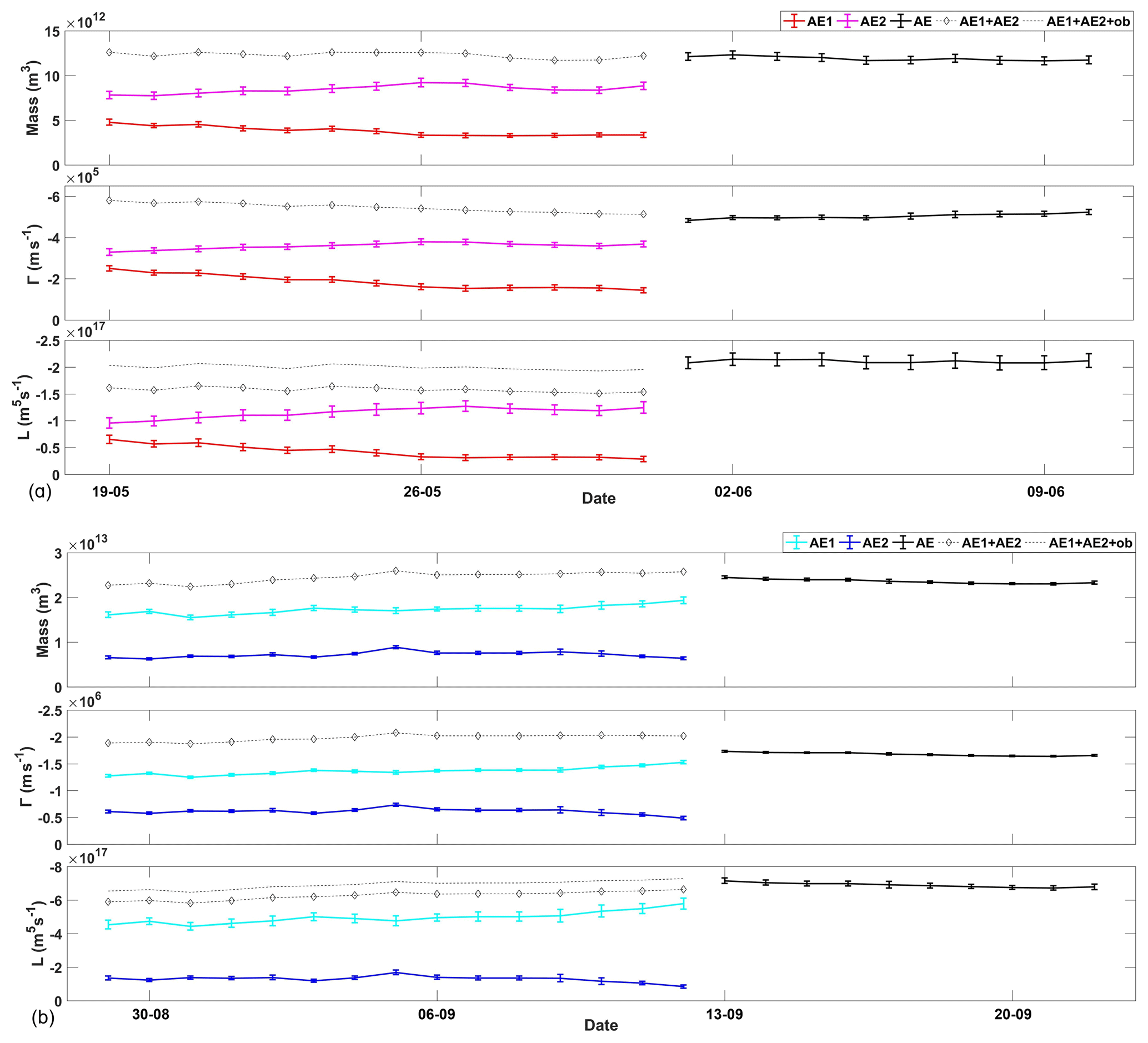
Figure 7There are two panels. The eddy properties (mass, circulation, and angular momentum) with a larger lateral boundary of integration in the merging event of (a) surface mesoscale eddies and (b) subsurface mesoscale eddies.
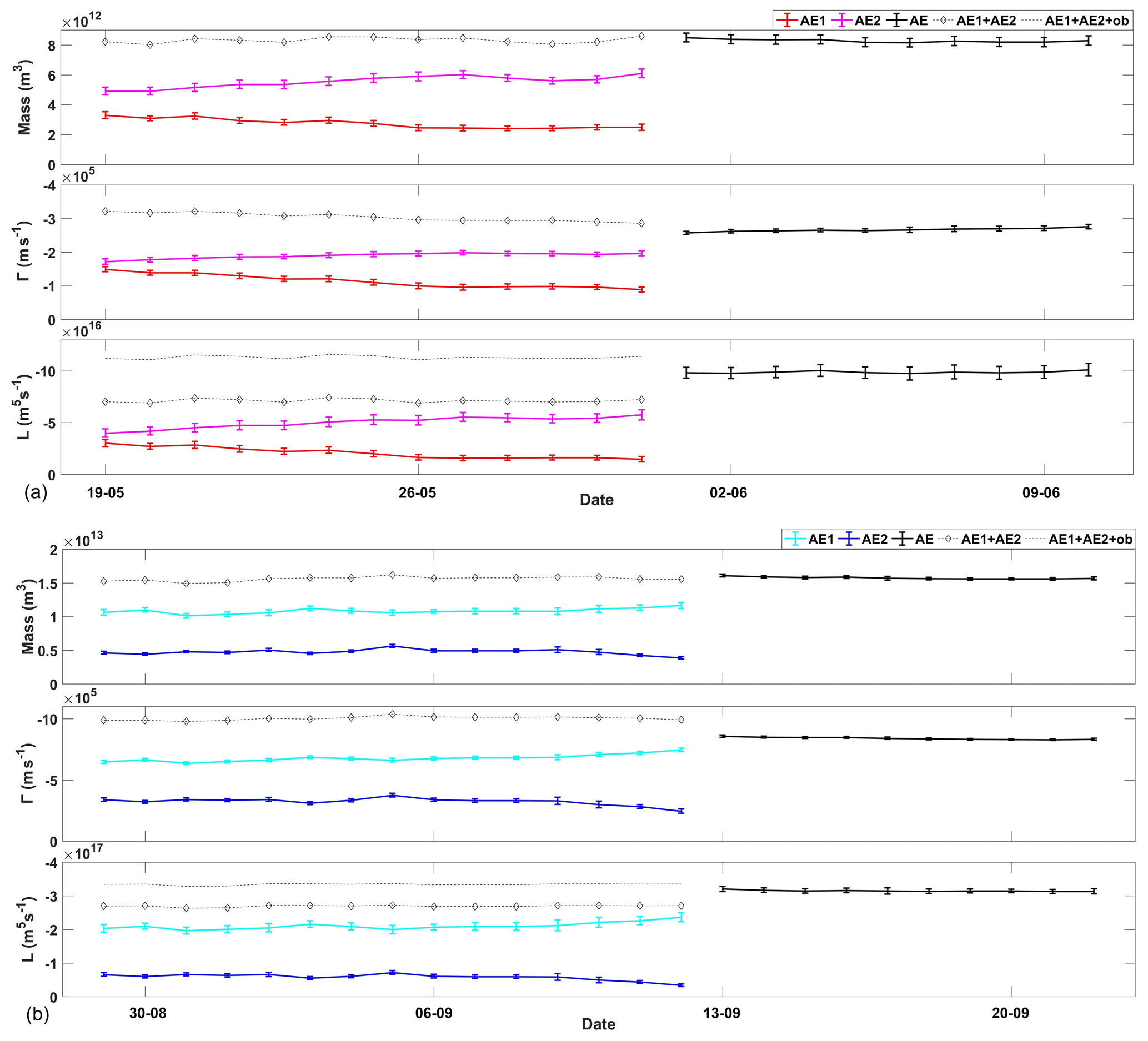
Figure 8The eddy properties (mass, circulation, and angular momentum) with a thicker H1=300 m in the merging event of (a) surface mesoscale eddies and (b) subsurface mesoscale eddies.
There is a long-standing question of which physical processes govern the seasonal variability of EKE (Marshall et al., 2002). The eddy merging process provides an effective means of mesoscale genesis, which might be a link in the chain of events. In the Northern Hemisphere (e.g., the Gulf Stream region and the Kuroshio extension region), the ocean is mostly baroclinically unstable in the mixed layer during late winter (Zhai et al., 2008; Qiu and Chen, 2010), when large-scale atmospheric forcing induces submesoscale eddies via mixed-layer instabilities (Sasaki et al., 2014). The surface ocean then becomes strongly stratified due to surface heating and weak vertical mixing in summer (Zhai et al., 2008; Ma et al., 2016). This strong stratification provides a large PE support for eddy mergers. Eddy merging events can pump the energy from submesoscale eddies into mesoscale eddies, in which it persists due to weaker dissipation. Consequently, EKE peaks in summer, as observed in previous studies (Zhai et al., 2008; Sasaki et al., 2014). Meanwhile, the submesoscale eddy condition itself usually has a seasonality, which affects the mesoscale eddy condition by inverse cascading (Yu et al., 2019). The strong eddy activity in turn modulates the mixed-layer depth (Gaube et al., 2019) and the isopycnals (Su et al., 2014).
4.1 Sensitivity to parameters
Firstly, there may be some concern about the sensitivity of the results to the choice of the lateral boundary of integration. Because we used optimally fitted intrinsic parameters other than the originally identified boundaries (e.g., Figs. 2 and 4) for integration, the results are insensitive to the identified eddy boundaries. In addition, the SLA (and vorticity) contour lines are self-similar ellipses according to the eddy model in Eq. (1), so the lateral boundary of integration was chosen as an ellipse. The conservation relationships are insensitive to the choice of the ellipse. For example, if we extend the integration region to a larger self-similar ellipse with a boundary satisfying ξ=0, the integration properties of both sides (before merger and after merger) synchronously become larger with nearly the same ratio (Fig. 7).
Secondly, there may also be a concern about how sensitive the results are to the choice of H1, as H1 was chosen as 200 m in the present study. Thus, we recalculated the eddy properties with the same eddy parameters obtained from the SLA field and density profile according to GODAS data, but simply enlarged H1 from 200 to 300 m while retaining the other parameters (including h1 and h2). The results are illustrated in Fig. 8. It is obvious that the total mass, total circulation, and total AM are hardly changed. Among these, the circulation seems more sensitive to the choice of H1. This is true because the circulation depends on both the surface parameters and also the vertical parameters (H1, h1, and h2) as the PV in Eq. (4). This might be the most sensitive case. In a more realistic scenario, a larger H1 would decrease the density difference ρ2−ρ1 between the lower levels H1 and H2, which consequently would lead to a larger h2. Thus, the PV in Eq. (4) should be less sensitive to H1 due to the compensation of h2.
In contrast to previous simple models, there are six eddy parameters – three horizontal (A, Lx, and Ly) and three vertical (H1, h1, and h2) in the present model. Two additional eddy parameters referring to the background – vertical shift b and angular speed ω – are also used. The additional degrees of freedom were expected to solve the dilemma of parameters being less numerous than conservation laws. All of the potential conservation laws were expected to hold simultaneously under the condition of more degrees of freedom than conservation laws. However, only limited conservation laws were found in the present results. It is noted that eddy conservation and conversion laws depend on the laws of physical dynamics, even if additional degrees of freedom can be provided in a mathematical model. This implies that the previous theoretical studies should be fully revisited because the physical conservation laws and physical properties were not correctly applied in these studies.
Although only eddy merging events were investigated in this study, it can be hypothesized that similar conservation and conversion laws are also valid in eddy splitting processes. The main difference may be that a physical quantity that ascends in the merging process, descends in the splitting process, and vice versa (Table 1). This hypothesis is partly supported by a previous numerical study. In a circulation-preserved flow field, a large eddy would split into small ones if energy decreased (Carnevale and Vallis, 1990). Moreover, there are other causes (e.g., instability processes of the eddy itself and interaction with external flow) that may lead to eddy merging and splitting processes. In such processes, the conservation and conversion laws may be quite different from those in Table 1.
4.2 Vertical merger
In the section above, we examined the evolution of two subsurface anticyclones in 2015 during a merger event. As both AEs were subsurface eddies, one wonders whether it is a stacking process or whether the two cores coalesce. The stacking process is different from the two cores coalescing in two ways. The first is eddy area. In a stacking process, the area of the final eddy would be significantly smaller than the summed area of the two eddies. If two cores coalesce, the area of the final eddy would be nearly the sum of the two eddies because the water of both eddies coalesces. The second one is AM. In a stacking process, the AM of the final eddy would nearly be the sum of the two eddies. In the case of two cores coalescing, the AM of the final eddy would be significantly larger than the sum of two eddies due to orbital AM. The above eddy mergers satisfy such properties, so they are more like two cores coalescing than a stacking process. As both eddies were located at the same depth before their merger, the eddy merging events in this study should be considered to be the horizontal merging type.
Additionally, there is a vertical merging type in which eddies are located at different depths before their merger. For example, Cresswell (1982) reported two warm-core eddies, Maria and Leo, located at 110–190 and 280–470 m depth, respectively. Eddy Maria overlapped eddy Leo in a stacking-like process, and the two eddies finally coalesced. As there are so many surface and subsurface eddies in the ocean, such merging types should also be common in nature. However, understanding how eddy properties satisfy the conservation and conversion laws after merger remains a challenge.
Finally, there are some interesting problems associated with the present study. How does a subsurface eddy move vertically, and which eddy properties are preserved during the motion? These problems have seldom been considered as only horizontal motions (and/or transports) of eddies were considered in the previous studies. Similarly to its horizontal motion, the vertical motion of an eddy might contribute to vertical transports and vertical mixing. This hypothesis should be studied further in the future.
In this paper, the theoretical “energy paradox” of whether the final state of two merging anticyclones contains more energy than the initial state was studied by observation of two cases of eddy merger. Conservation laws of mass, total circulation, and AM were examined using a two-layer model and parameters obtained by fitting to observations. While the conservation laws of mass and total circulation were satisfied with the eddy parameters, the conservation of AM required inclusion of the orbital AM. Both the conservation of circulation and the orbital AM were overlooked in previous theoretical studies.
In contrast, neither the EKE nor the EPE was conserved after merging. The EKE decreased due to fusion and the EPE increased due to environmental PE conversion related to the vertical shift parameter b. The total mechanical energy increased after merging. According to the present results, we can answer the energy paradox: the final merged eddy has more energy than the initial state eddies, and the energy is mainly contributed from background gravitational PE below the eddies, which is converted to EPE. In addition, eddy merging behaves like a “large-scale energy pump” in inverse energy cascades, which plays an important role in ocean dynamics.
Finally, the merging and splitting of eddies do not change the total mass, circulation, and AM of the flow field system, but they do change the energy distributions and portions in different scales, which is essential for the energy cascade in multiscale fluid dynamics.
The SLA data are produced and distributed by AVISO (https://www.aviso.altimetry.fr/, Pujol et al., 2016). The SST data were downloaded at APDRC (http://apdrc.soest.hawaii.edu/data/, Donlon et al., 2012). The ocean vertical density profile data were downloaded from NOAA (https://www.esrl.noaa.gov/psd/data/gridded/data.godas.html, Behringer et al., 2004). The eddy detection method and the code can be downloaded from Ocean Science (https://doi.org/10.5194/os-12-1249-2016, Li et al., 2016).
LS designed the research; ZFW and LS performed the research; QYL and HC contributed data; ZFW and HC drew figures; and LS and ZFW wrote the paper.
The authors declare that they have no conflict of interest.
We thank the reviewers and the editor for their useful comments, and we also thank Wei Wang at OUC for useful discussions. This work was supported by the National Foundation of Natural Science of China (no. 41876013) and the National Programme on Global Change and Air–Sea Interaction (GASI-IPOVAI-04).
This research has been supported by the National Foundation of Natural Science of China (grant no. 41876013) and the National Programme on Global Change and Air–Sea Interaction (grant no. GASI-IPOVAI-04).
This paper was edited by Ilker Fer and reviewed by two anonymous referees.
Amores, A., Jordà, G., Arsouze, T., and Le Sommer, J.: Up to what extent can we characterize ocean eddies using present-day gridded altimetric products?, J. Geophys. Res.-Oceans, 123, 7220–7236, 2018.
Assassi, C., Morel, Y., Vandermeirsch, F., Chaigneau, A., Pegliasco, C., Morrow, R., Colas, R., Fleury, S., Carton, X., and Klein, P.: An index to distinguish surface-and subsurface-intensified vortices from surface observations, J. Phys. Oceanogr., 46, 2529–2552, 2016.
Ballarotta, M., Ubelmann, C., Pujol, M.-I., Taburet, G., Fournier, F., Legeais, J.-F., Faugère, Y., Delepoulle, A., Chelton, D., Dibarboure, G., and Picot, N.: On the resolutions of ocean altimetry maps, Ocean Sci., 15, 1091–1109, https://doi.org/10.5194/os-15-1091-2019, 2019.
Bashmachnikov, I. L., Sokolovskiy, M. A., Belonenko, T. V., Volkov, D. L., Isachsen, P. E., and Carton, X.: On the vertical structure and stability of the Lofoten vortex in the Norwegian Sea, Deep-Sea Res. Pt. I, 128, 1–27, 2017.
Behringer, D. W. and Xue, Y.: Evaluation of the global ocean data assimilation system at NCEP: The Pacific Ocean[C]//Proc. Eighth Symp. on Integrated Observing and Assimilation Systems for Atmosphere, Oceans, and Land Surface, Seattle, Wash: AMS 84th Annual Meeting, Washington State Convention and Trade Center, 11–15 January 2004 (data available at: https://www.esrl.noaa.gov/psd/data/gridded/data.godas.html, last access: 18 November 2019).
Bosse, A., Fer, I., Søiland, H., and Lilly, J. M.: Dynamical controls on the longevity of a non-linear vortex: The case of the Lofoten Basin Eddy, Sci. Rep., 9, 13448, https://doi.org/10.1038/s41598-019-49599-8, 2019.
Carnevale, G. F. and Vallis, G. K.: Pseudo-advective relaxation to stable states of inviscid two-dimensional fluids, J. Fluid Mech., 213, 549–571, 1990.
Chelton, D. B., Schlax, M. G., and Samelson, R. M.: Global observations of nonlinear mesoscale eddies, Prog. Oceanogr., 91, 167–216, 2011.
Chen, G., Han, G., and Yang, X.: On the intrinsic shape of oceanic eddies derived from satellite altimetry, Remote Sens. Environ., 228, 75–89, 2019.
Cui, W., Wang, W., Zhang, J., and Yang, J.: Multicore structures and the splitting and merging of eddies in global oceans from satellite altimeter data, Ocean Sci., 15, 413–430, https://doi.org/10.5194/os-15-413-2019, 2019.
Cushman-Roisin, B.: On the role of filamentation in the merging of anticyclonic lenses, J. Phys. Oceanogr., 19, 253–258, 1989.
Cresswell, G. R.: The coalescence of two East Australian Current warm-core eddies, Science, 215, 161–164, 1982.
Dong, C., McWilliams, J. C., Liu, Y., and Chen, D.: Global heat and salt transports by eddy movement, Nat. Commun., 5, 3294, https://doi.org/10.1038/ncomms4294, 2014.
Donlon, C. J., Martin, M., Stark, J., Roberts-Jones, J., Fiedler, E., and Wimmer, W.: The operational sea surface temperature and sea ice analysis (OSTIA) system, Remote Sens. Environ., 116, 140–158, 2012 (data available at: http://apdrc.soest.hawaii.edu/data/, last acess: 18 November 2019).
Ducet, N., Le Traon, P. Y., and Reverdin, G.: Global high-resolution mapping of ocean circulation from TOPEX/Poseidon and ERS-1 and-2, J. Geophys. Res.-Oceans, 105, 19477–19498, 2000.
Gaube, P., McGillicuddy Jr., D. J., and Moulin, A. J.: Mesoscale eddies modulate mixed layer depth globally, Geophys. Res. Lett., 46, 1505–1512, 2019.
Gill, A. E.: Atmosphere–Ocean Dynamics, Academic Press, 662 pp., 1982.
Griffiths, R. W. and Hopfinger, E. J.: Coalescing of geostrophic vortices, J. Fluid Mech., 178, 73–97, 1987.
Klein, P., Lapeyre, G., Siegelman, L., Qiu, B., Fu, L., Torres, H., Su, Z., Menemenlis, D., and Gentil, S.: Ocean-Scale Interactions From Space, Earth and Space Science, 6, 795–817, 2019.
Laxenaire, R., Speich, S., Blanke, B., Chaigneau, A., Pegliasco, C., and Stegner, A.: Anticyclonic eddies connecting the western boundaries of Indian and Atlantic Oceans, J. Geophys. Res.-Oceans, 123, 7651–7677, 2018.
Li, C., Zhang, Z., Zhao, W., and Tian, J.: A statistical study on the subthermocline submesoscale eddies in the northwestern Pacific Ocean based on Argo data, J. Geophys. Res.-Oceans, 122, 3586–3598, 2017.
Li, Q., Sun, L., Liu, S., et al.: A new mononuclear eddy identification method with simple splitting strategies, Remote Sens. Lett., 5, 65–72, 2014.
Li, Q., Sun, L., and Xu, C.: The Lateral Eddy Viscosity Derived from the Decay of Oceanic Mesoscale Eddies, Open Journal of Marine Science, 8, 152–172, 2018.
Li, Q. Y. and Sun, L.: Technical Note: Watershed strategy for oceanic mesoscale eddy splitting, Ocean Sci., 11, 269–273, https://doi.org/10.5194/os-11-269-2015, 2015.
Li, Q.-Y., Sun, L., and Lin, S.-F.: GEM: a dynamic tracking model for mesoscale eddies in the ocean, Ocean Sci., 12, 1249–1267, https://doi.org/10.5194/os-12-1249-2016, 2016.
Lumpkin, R., Flament, P., Kloosterziel, R., and Armi, L.: Vortex Merging in a 1 1/2-Layer Fluid on an f Plane, J. Phys. Oceanogr., 30, 233–242, 2000.
Ma, X., Jing, Z., Chang, P., Liu, X., Raffaele, M., Justin, S., Frank, B., Richard, G., Peter, B., and Wu, D.: Western boundary currents regulated by interaction between ocean eddies and the atmosphere, Nature, 535, 533–537, 2016.
Marshall, J., Jones, H., Karsten, R., and Wardle, R.: Can eddies set ocean stratification?, J. Phys. Oceanogr., 32, 26–38, 2002.
Mason, E., Ruiz, S., Bourdalle-Badie, R., Reffray, G., García-Sotillo, M., and Pascual, A.: New insight into 3-D mesoscale eddy properties from CMEMS operational models in the western Mediterranean, Ocean Sci., 15, 1111–1131, https://doi.org/10.5194/os-15-1111-2019, 2019.
McGillicuddy, D, J.: Eddies masquerade as planetary waves, Science, 334, 318–319, 2011.
Nof, D.: The fusion of isolated nonlinear eddies, J. Phys. Oceanogr., 18, 887–905, 1988.
Nof, D.: The role of angular momentum in the splitting of isolated eddies, Tellus A, 42, 469–481, 1990.
Nof, D. and Simon, L. M.: Laboratory experiments on the merging of nonlinear anticyclonic eddies, J. Phys. Oceanogr., 17, 343–357, 1987.
Pavia, E. G. and Cushman-Roisin, B.: Merging of frontal eddies, J. Phys. Oceanogr., 20, 1886–1906, 1990.
Pujol, M.-I., Faugère, Y., Taburet, G., Dupuy, S., Pelloquin, C., Ablain, M., and Picot, N.: DUACS DT2014: the new multi-mission altimeter data set reprocessed over 20 years, Ocean Sci., 12, 1067–1090, https://doi.org/10.5194/os-12-1067-2016, 2016 (data available at: https://www.aviso.altimetry.fr/, last access: 18 November 2019).
Qiu, B. and Chen, S.: Eddy-mean flow interaction in the decadally modulating Kuroshio Extension system, Deep-Sea Res. Pt. II, 57, 1098–1110, 2010.
Qiu, B., Nakano, T., Chen, S., nd Klein, P.: Submesoscale transition from geostrophic flows to internal waves in the northwestern Pacific upper ocean, Nat. Commun., 8, 14055, https://doi.org/10.1038/ncomms14055, 2017.
Raj, R. P., Johannessen, J. A., Eldevik, T., Nilsen, J. E. Ø., and Halo, I.: Quantifying mesoscale eddies in the lofoten basin, J. Geophys. Res.-Oceans, 121, 4503–4521, 2016.
Sangrà, P., Pelegrí, J. L., Hernández-Guerra, A., Arregui, I., Martín, J. M., Marrero‐Díaz, A., Martínez, A., Ratsimandresy, A. W., and Rodríguez-Santana, A.: Life history of an anticyclonic eddy, J. Geophys. Res.-Oceans, 110, 2156–2202, 2005.
Sasaki, H., Klein, P., Sasai, Y., and Qiu, B.: Regionality and seasonality of submesoscale and mesoscale turbulence in the North Pacific Ocean, Ocean Dynam., 67, 1195–1216, 2017.
Schultz Tokos, K. L., Hinrichsen, H. H., and Zenk, W.: Merging and migration of two meddies, J. Phys. Oceanogr., 24, 2129–2141, 1994.
Su, Z. and Ingersoll, A. P.: On the minimum potential energy state and the eddy size–constrained APE density, J. Phys. Oceanogr., 46, 2663–2674, 2016.
Su, Z., Stewart, A. L., and Thompson, A. F.: An idealized model of Weddell Gyre export variability, J. Phys. Oceanogr., 44, 1671–1688, 2014.
Su, Z., Wang, J., Klein, P., Thompson, A. F., and Menemenlis, D.: Ocean submesoscales as a key component of the global heat budget, Nat. Commun., 9, 775, https://doi.org/10.1038/s41467-018-02983-w, 2018.
Torres, H. S., Klein, P., Menemenlis, D., Qiu, B., Su, Z., Wang, J., Chen, S., and Fu, L.: Partitioning ocean motions into balanced motions and internal gravity waves: A modeling study in anticipation of future space missions., J. Geophys. Res.-Oceans, 123, 8084–8105, 2018.
Wang, Q.: Three-dimensional structure of mesoscale eddies in the western tropical Pacific as revealed by a high-resolution ocean simulation, Sci. China Earth Sci., 9, 155–167, 2017.
Wang, Z., Li, Q., Sun, L., Li, S., Yang, Y., and Liu, S.: The most typical shape of oceanic mesoscale eddies from global satellite sea level observations, Front. Earth Sci., 9, 202–208, 2015.
Wu, J. Z., Ma, H. Y., and Zhou, M. D.: Vorticity and vortex dynamics, Springer Science & Business Media, 2007.
Xu, C., Shang, X. D., and Huang, R. X.: Horizontal eddy energy flux in the world oceans diagnosed from altimetry data, Sci. Rep., 4, 5316, https://doi.org/10.1038/srep05316, 2014.
Yang, Z., Wang, G., and Chen, C.: Horizontal velocity structure of mesoscale eddies in the South China Sea, Deep-Sea Res., 149, 103055, https://doi.org/10.1016/j.dsr.2019.06.001, 2019.
Yi, J., Du, Y., Zhou, C., Liang, F., and Yuan, M.: Automatic identification of oceanic multieddy structures from satellite altimeter datasets, IEEE J. Sel. Top. Appl., 8, 1555–1563, 2015.
Yu, X., Naveira Garabato, A. C., Martin, A. P., Liang, F., and Yuan, M.: An annual cycle of submesoscale vertical flow and restratification in the upper ocean, J. Phys. Oceanogr., 49, 1439–1461, 2019.
Zhai, X., Greatbatch, R. J., and Kohlmann, J. D.: On the seasonal variability of eddy kinetic energy in the Gulf Stream region, Geophys. Res. Lett., 35, 745–750, 2008.
Zhang, Z., Wang, W., and Qiu, B.: Oceanic mass transport by mesoscale eddies, Science, 345, 322–324, 2014.
Zhang, Z., Li, P., Xu, L., Li, C., Zhao, W., Tian, J., and Qu, T.: Subthermocline eddies observed by rapid-sampling Argo floats in the subtropical northwestern Pacific Ocean in Spring 2014, Geophys. Res. Lett., 42, 6438–6445, 2015.
Zhang, Z., Qiu, B., Klein, P., and Travis, S.: The influence of geostrophic strain on oceanic ageostrophic motion and surface chlorophyll, Nat. Commun., 10, 2838, https://doi.org/10.1038/s41467-019-10883-w, 2019.
paradoxabout the merging of two anticyclonic mesoscale eddies is studied. While the conservation laws of mass and total circulation were satisfied, the conservation of AM required inclusion of the orbital AM. Both the conservation of circulation and the orbital AM were overlooked in previous theoretical studies. The eddy kinetic energy decreased due to fusion, but the eddy potential energy increased. This behaves like a
large-scale energy pumpin inverse energy cascades.
paradoxabout the merging of two anticyclonic mesoscale eddies is studied. While...