the Creative Commons Attribution 4.0 License.
the Creative Commons Attribution 4.0 License.
 | 10 Dec 2019
Depth is relative: the importance of depth for transparent exopolymer particles in the near-surface environment
Tiera-Brandy Robinson
Christian Stolle
Oliver Wurl
Transparent exopolymer particles (TEPs) are a major source for both organic matter (OM) and carbon transfer in the ocean and into the atmosphere. Consequently, understanding the vertical distribution of TEPs and the processes which impact their movement is important in understanding the OM and carbon pools on a larger scale. Additionally, most studies looking at the vertical profile of TEPs have focused on large depth scales from 5 to 1000 m and have omitted the near-surface environment. Results from a study of TEP enrichment in the sea surface microlayer (SML) in different regions (tropical, temperate) has shown that, while there is a correlation between TEP concentration and primary production (PP) on larger or seasonal scales, such relationships break down on shorter timescales and spatial scales. Using a novel small-scale vertical sampler, the vertical distribution of TEPs within the uppermost 2 m was investigated. For two regions with a total of 20 depth profiles, a maximum variance of TEP concentration of 1.39×10⁶ µg XG eq2 L−2 between depths and a minimum variance of 6×10² µg XG eq2 L−2 was found. This shows that the vertical distribution of TEPs was both heterogeneous and homogeneous at times. Results from the enrichment of TEPs and Chl a between different regions have shown TEP enrichment in the SML to be greater in oligotrophic waters, when both Chl a and TEP concentrations were low, suggesting the importance of abiotic sources for the enrichment of TEPs in the SML. However, considering multiple additional parameters that were sampled, it is clear that no single parameter could be used as a proxy for TEP heterogeneity. Other probable biochemical drivers of TEP transport are discussed.
- Article
(2740 KB) -
Supplement
(206 KB) - BibTeX
- EndNote


The sea surface microlayer (SML), a thin layer 10 µm–1 mm thick, lays at the top of the ocean. It has distinct chemical, biological and physical properties (Sieburth, 1983; Cunliffe et al., 2013; Wurl et al., 2016) setting it apart from underlaying water (ULW). As the boundary layer between the ocean and atmosphere, it significantly controls the flux of such important substances as CO2 and organic matter (OM) (Wurl et al., 2016; Engel et al., 2017).
The SML is further characterized by its gelatinous nature (Sieburth, 1983), being thoroughly permeated with extracellular polymeric substances, the largest faction of which are transparent exopolymer particles (TEPs) (Wurl and Holmes, 2008; Cunliffe and Murrell, 2009). These gel particles can form in two ways: abiotically via the collision of colloidal material by physical forces or biotically via the breakdown and secretion of precursor material from organisms, with phytoplankton being the largest source (Passow, 2002a). These gels are “sticky” by nature and thus can aggregate to themselves but also to other solid particles, making them a large source for the transport of OM in the ocean (Passow, 2002b). Unattached, TEPs have a low density and are positively buoyant (Azetsu-Scott and Passow, 2004), so that unless enough highly dense matter (e.g. mineral, phytoplankton cells, fecal pellets) is attached or a dense enough aggregate is formed to cause sinking, these aggregates will rise to the surface and help to form the SML (Wurl and Holmes, 2008). Meanwhile, when these OM-rich aggregates sink, they help to feed the chemical pump via increased input of dissolved inorganic carbon. The chemical pump is highly dependent on seawater temperature and thermohaline circulation and uses increased solubility of carbon in cooler water to “pump” carbon from the surface to deeper waters. On a larger scale, these OM-rich aggregates also feed the biological pump not only because of their increased total input of dissolved and particulate organic matter, but due to their increased sinking velocity, these aggregates have a reduced chance of remineralization and therefore it increases the downward flux of carbon and its sequestering to the sea floor. (Mari et al., 2017; Engel, 2004). Due to the role of TEPs in OM and carbon fluxes both within the ocean and into the atmosphere, it is important to understand what parameters can enhance TEP distribution and enrichment in the ocean. Additionally, because TEPs are a part of a complex biochemical process, cross-regional examination of TEPs can help to understand underlying characteristics of TEPs.
There have been multiple studies which have looked at the vertical distribution of TEPs in the ocean to understand the rising and sinking of these aggregates and their relation to other parameters (Ortega-Retuerta et al., 2017; Busch et al., 2017; Kodama et al., 2014; Wurl et al., 2011a; Cisternas-Novoa et al., 2015; Yamada et al., 2017). However, until recently, most studies have focused on large-scale vertical distributions beginning at 5 m and going to thousands of metres depth, and always considered the top 5–10 m of the ocean as homogenous. As the importance of the SML in air–sea exchanges has grown (Liss et al., 2005; Cunliffe et al., 2013; Wurl et al., 2017), more studies have begun to investigate the relationship and enrichment of the SML in comparison with underlaying water (ULW). To date, there is no consistent measuring depth for what is termed ULW; it is dependent solely on the individual setup of the researchers but is often operationally defined at 1 m.
The purpose of this study was to understand if there are single drivers of TEP vertical distribution in the upper 2 m and if these drivers are consistent between regions. To accomplish this, we investigated the abundance and enrichment of TEPs between the SML and ULW, in various regions of the ocean and its relation to biochemical factors. A further aim was to determine if 1 m depth is a good reference for TEPs and other parameters, and how important depth is in sampling within the top 2 m. We present data from three field campaigns which show the accumulation of TEPs in the upper 2 m and how they relate to water column stratification, primary production and sea surface conditions.
2.1 Study areas
Water samples were collected as part of the MarParCloud project Cabo Verde campaign in the nearshore water in São Vicente, on the research cruise HE491 in the North Sea/Norwegian Sea and fjords, and from the research cruise EMB184 in the Baltic Sea (Fig. 1). The sampling areas represent uniquely different regions; São Vicente has oligotrophic tropical water with large influences from Saharan dust deposition, the Norwegian fjords and Baltic Sea are both temperate climates, but the inner and outer Norwegian fjord systems have a large interaction with North Atlantic water, while the Baltic Sea is semi-enclosed with larger anthropological interaction and little interaction with North Atlantic water.
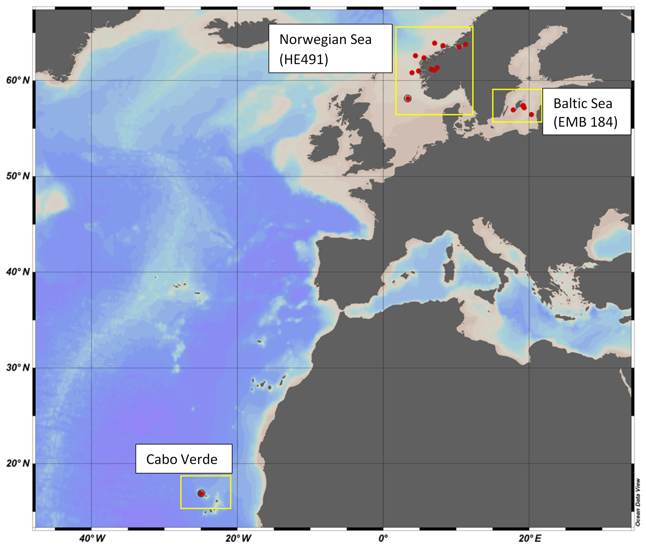
Figure 1Map showing field campaign areas and stations.
2.2 Sampling: Norwegian Sea (HE498) and Baltic Sea (EMB184) research cruises
North Sea/Norwegian Sea and fjord samples were collected between 8 and 25 July 2017 aboard the R/V Heinke. Samples were collected once per day, weather permitting, from each station, with a total of 13 stations spanning inner fjord, outer fjord and open-ocean areas. Samples were collected from both the North Sea and the Norwegian Sea, but for the purpose of clarity, that campaign will be termed the “Norwegian Sea” campaign. Baltic Sea samples were collected between 30 May and 10 June 2018 aboard the R/V Elisabeth Mann Borgese, with a total of eight stations used. SML and ULW samples were collected using the radio-controlled sea surface scanner (S3), as described in Ribas-Ribas et al. (2017), which has six rotating glass discs partially immersed in the water to sample the SML by its surface tension. ULW (1 m depth) and SML water were pumped through two separate flow-through systems with onboard sensors at a rate of 1.2 L min−1 using peristaltic pumps. SML and ULW water are collected in 1 L bottles by the pilot's command and in addition collected into large volume carboys. Large sample volumes (∼20 L) were collected for multiple analyses by all groups involved in the campaigns. The S3 also records multiple meteorological parameters: photosynthetically active radiation (PAR), solar radiation, wind speed and humidity. Salinity was measured on SML and ULW using a multi-parameter meter (MU 6100 H, VWR) before the collection of the sample into a container; high-precision in situ temperature was constantly measured for the SML and ULW using a reference thermometer (P795, Dostmann Electronics GmbH). Specifications for instrument precision and accuracy can be found in Ribas-Ribas et al. (2017). All in situ data were averaged for the 2 h surrounding the sampling of discrete water samples. A new device termed the High-volume Sampler for the Vertical (HSV) was deployed to collect water from five depths between the SML and 2 m. The HSV is made of a vertical polypropylene pipe with five polypropylene tubes set at five distinct depths in the pipe and a float attached to the top which has been ballasted to ensure accuracy in depth. Peristaltic pumps, similar to that on the S3, pump water into collection containers. The HSV was deployed during the collection time of discrete SML and ULW samples by the S3 and close enough to the S3 so that it would sample the same body of water but would not interfere with the glass plate sampling.
2.3 Sampling: Cabo Verde
Samples were taken once a day, weather permitting, between 18 September and 6 October 2016 within the same nearshore water (∼1 km), with a total of 12 stations sampled. SML and ULW samples were collected from fisher boats in the nearshore waters. SML samples were collected using the glass plate technique (Harvey and Burzell, 1972; Cunliffe and Wurl, 2014) and ULW was collected from 1 m depth using a large syringe. Wind speed was recorded using an anemometer placed at the nearby Cape Verde Atmospheric Observatory (CVOA) station. A handheld Global Position System (Garmin eTrex) was used to track fisher boat movement during sampling and for coordinates of each sampling station.
2.4 POC, PON, POP and nutrients
Samples for particulate organic carbon (POC), nitrogen (PON) and phosphorous (POP) were filtered onto acid-washed and precombusted glass-fibre filters (Whatman GF/C). Filters for POC and PON were dried at 60 ∘C for 3 d (Norwegian cruise) or 130 ∘C for 2 h (Baltic cruise and Cabo Verde), put in tin capsules and measured using an elemental analyser (Thermo, Flash EA 1112 and Elementar Analysensysteme, precision of 0.01±0.2 ‰). POP was measured by molybdate reaction after digestion with potassium peroxydisulfate (K2S2O8) solution (Wetzel and Likens, 2000). The filtered water was collected and analysed for dissolved nutrients (PO4, NO3) by a continuous-flow analyser according to Grasshoff et al. (1999).
2.5 Chlorophyll a
During the Cabo Verde and Baltic (EMB184) campaigns, chlorophyll a (Chl a) was measured by filtering 500–1000 mL of seawater onto precombusted (4 h, 450 ∘C) GF/F filters (Whatman). The filters were stored frozen (−18 ∘C) until processed. Chl a was then analysed according to the method described by Wasmund et al. (2006) using a fluorometer (Jenway 6285, precision of 0.01± < 1 ng mL−1). During the Norwegian cruise (HE491), in vivo Chl a was measured with a hand fluorometer (Turner Designs, AquaFluorTM, precision of 0.001 absorption) and related to µg of Chl a using a calibration factor between filtered Chl a (Chl a standard in EtOH as reference) and in vivo absorbance.
2.6 Bacterial cell numbers (only for Baltic cruise)
The total cell numbers (TCNs) of prokaryotic and small autotrophic cells were determined by flow cytometry following a modified protocol from Marie et al. (2000). For determination of bacterial cell numbers, water samples were fixed with glutaraldehyde (1 % final concentration), incubated at room temperature for 1 h and stored at C until further analysis. Prokaryotic cells were stained with SYBR Green I (2.5 mM final concentration, Molecular Probes, Schwerte, Germany) for 30 min in the dark. Samples were measured on a flow cytometer (C6 FlowCytometer, BD Bioscience, fluorescence accuracy of FITC (fluorescein isothiocyanate) < 75; PE (phycoerythrin) < 50), and cells were counted according to side-scattered light and emitted green fluorescence. We used 1.0 µm beads (Fluoresbrite Multifluorescent, Polysciences) as an internal reference to monitor the performance of the device. Their cell counts include heterotrophic and photoautotrophic prokaryotes. Pico- and nano-autotrophic cells were counted after the addition of red fluorescent latex beads (Polysciences, Eppelheim, Germany) and were detected by their signature in a plot of red (FL3) vs. orange (FL2) fluorescence, and red fluorescence vs. side scatter (SSC). We did not further differentiate between different groups of prokaryotic and eukaryotic autotrophs.
2.7 TEPs
TEPs were measured by filtering seawater, in triplicates, onto 0.2 µm polycarbonate filters under low vacuum (< 100 mm Hg) and staining with alcian blue solution (0.02 g alcian blue in 100 mL of acetic acid solution of pH 2.5) for 5 s. The 0.2 µm filters collect both large TEP aggregates and smaller colloidal TEP material. Filters were stored at −18 ∘C until processed. Alcian blue stain was extracted for 2 h in 80 % sulfuric acid, with gentle agitation applied to reduce bubble formation, and analysed using a spectrophotometer (VWR UV-1600PC, precision of 1±0.2 % T) and the spectrophotometric method (Passow and Alldredge, 1995). The stock solution of alcian blue was calibrated using the xanthan gum (Carl Roth) standard according to Passow and Alldredge (1995). TEP concentrations are shown in relation to xanthan gum equivalence. Recent calibration issues with xanthan gum were not observed in our studies, and thus the new method by Bittar et al. (2018) was not required.
2.8 Primary production
To estimate local primary production, we used an adjusted version of the Vertically Generalized Production Model (VGPM) (Behrenfeld and Falkowski, 1997), as described by Wurl et al. (2011b). Estimation is based on concentration of Chl a, depth of euphotic zone estimated from the Secchi depth, photoperiod and photosynthetic active radiation (PAR).
2.9 Data analysis
Statistical analyses of the data set were performed using Graphpad PRISM version 8. Differences, null hypothesis testing, and correlation were considered significant when p < 0.05. The data were log transformed, if required, for parametric and analysis of variance (ANOVA) tests; further post-hoc Tukey analysis was run for comparison of means when the difference was significant in ANOVA. Unless otherwise indicated, results are presented as means ± standard deviations. Enrichment factors (EFs) were calculated as the ratio of concentrations in the SML sample to that of corresponding ULW taken at 1 m depth. For vertical sample profiles, the variance of each depth measurement from the average was used to determine homogeneity. Variance is the squared deviation from the mean of all depths and is thus given in units squared (e.g. µg2 L−2).

Figure 2Regional comparison of enrichment and SML concentrations for Chl a (a, b) and TEPs (c, d). The enrichment factor (EF) is given on the y axis for panels (a, c) and is given as the concentration in the SML over the concentration in the ULW. Horizontal lines are shown on panels (a, c) to distinguish varying levels of enrichment.
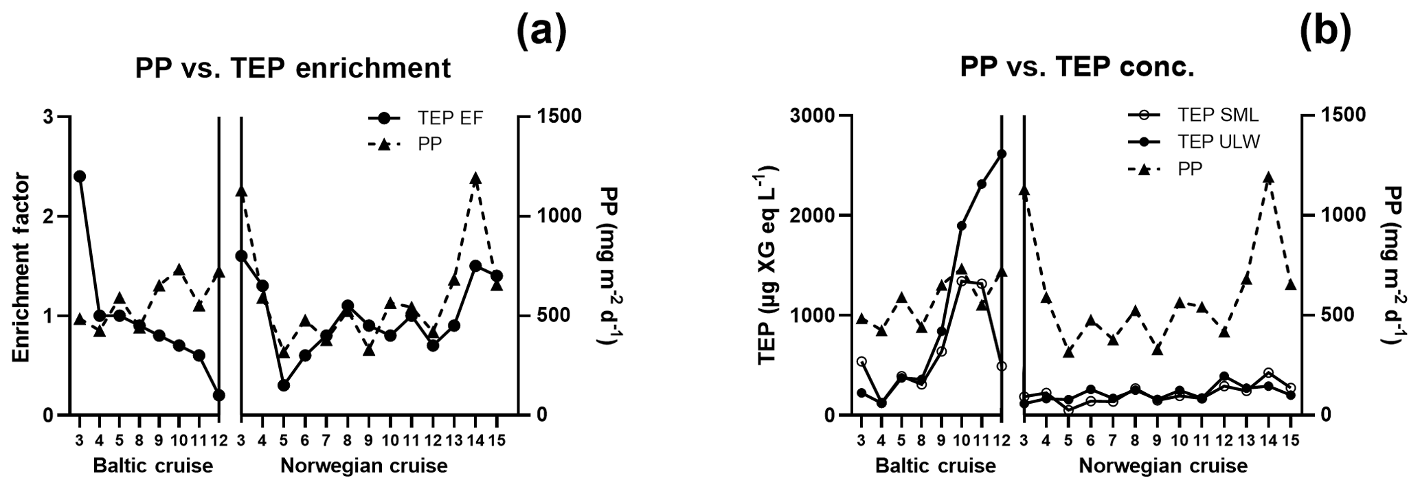
Figure 3Comparison of (a) TEP enrichment and (b) concentration with primary production (PP) along the cruise tracks for the Baltic and Norwegian cruises; numbers on the x axis denote station numbers.
3.1 General conditions
General characteristics of parameters for all three campaigns are shown in Figs. 2 and 3. We observed low (< 2 m s−1), moderate (2–5 m s−1) and high (> 5 m s−1) wind regimes (Wurl et al., 2011b). Average wind speed was 3.8±0.3, 4.2±2 and 5.6±1.8 m s−1 for the Baltic Sea, Norwegian Sea and Cabo Verde, respectively. PAR averages were 1172±145 and 739±251 µmol m−2 s−1 for the Baltic Sea and Norwegian Sea, respectively, and sea surface temperature (SST), measured from the SML, was 14.8±1.9 and 14.9±1.4 ∘C. Stations for the Baltic cruise were sampled within the same area (∼1 km) and thus had similar salinity (8.92±0.2) relative to those from the Norwegian cruise. The stations for the Norwegian cruise covered inner and outer fjord and open-ocean areas and thus had larger differences of salinity. SML salinity was (32.4±2; 23.5±0.4; 6.7±3.5) for outer fjord/open ocean, Trondheim fjord and Sognefjord, respectively. ULW salinity was 32.7±2, 23.9±0.2 and 6.6±3.5 for outer fjord/open ocean, Trondheim Fjord and Sognefjord, respectively. PAR, SST and salinity data were not collected for the Cabo Verde campaign due to logistical constraints. Primary production (PP) ranged from 426 to 734 mg m−2 d−1 during the Baltic cruise but had a higher range during the Norwegian cruise with 318–1194 mg m−2 d−1. Again, this is likely due to the differing water masses sampled during the Norwegian cruise.
3.2 TEP distribution in the SML across different regions
3.2.1 Baltic Sea
TEP concentrations ranged from 123 to 1340 µg XG eq L−1 in the Baltic Sea. Nitrate and phosphate levels were relatively higher compared to the other regions (nitrate: < 0.1 µmol L−1; phosphate: < 0.2 µmol L−1). The Baltic Sea was also marked with the highest levels of POC in the SML with a range of 27.4–274 µmol L−1. POC enrichment in the SML matched TEP and PON enrichment trends which showed EFs > 1 for stations 4–5 and EFs < 1 for stations 9–10. TEP enrichment factors were ≥1 for the first half of the cruise (stations 3–5) and < 1 for the second half of the cruise (stations 8–12). However, total TEP concentration in the SML and ULW increased substantially in the second half of the cruise (stations 9–12), with TEPs in the SML averaging 341±150 and in the ULW 269±104 µg XG eq L−1 at the beginning and in the SML 946±386 and in the ULW 1916±671 µg XG eq L−1 for the second half. Chl a was not enriched in the SML at any station, while Chl a concentrations ranged between 0.68 and 1.56 µg L−1, with the highest concentrations at stations 9 and 10. PP matched trends of TEPs except at station 11, which showed relatively low levels of Chl a (0.80 µg L−1) and a resulting decrease in PP (from 734 down to 553 mg−2 d−1) but relatively high levels of TEPs (2313 µg XG eq L−1) (Fig. 3b).
3.2.2 Norwegian Sea
TEP concentrations during the Norwegian cruise ranged from 50 to 424 µg XG eq L−1 and had geographically sporadic enrichment with 50 % of observations showing EF ≥1 and 50 % showing EF < 1. The highest enrichments were observed at station 3 (EF =1.6), which was the furthest open-ocean station, and stations 13 and 14 (EF =1.5; 1.4), which were in the Trondheim fjord. Nitrate and phosphate were both homogenously low for all stations (0.04±0.04; 0.07±0.03 µmol L−1). PON concentrations in the SML ranged 0.6–2 µmol L−1 and were never enriched, mainly due to low overall concentrations in the water. However, PON in the ULW was higher (> 1 µmol L−1) in both inner fjords compared to the outer fjord and open ocean (< 1 µmol L−1). POC in the ULW was also higher in both inner fjords (20.5±6.1 µmol L−1) compared to the outer fjord and open-ocean stations (10.7±1.1 µmol L−1). Similar to PON, POC in the SML showed no general enrichment and had EF < 1 for most stations except stations 3, 8 and 11. Chl a concentrations in the SML ranged from 0.29 to 1.64 µg L−1, with the lowest concentrations in the outer fjords and open-ocean stations and highest concentrations in the Trondheim fjord. Enrichment of TEPs and Chl a were both sporadic and did not have matching trends, with Chl a sometimes enriched when TEPs were not (stations 5 and 12) and TEPs enriched when Chl a was not (stations 14 and 15). However, this appears to be influenced by the fjord systems; when only the open-ocean and nearshore stations were considered, TEP and Chl a enrichment trends did match.
Table 1S3 data with averages ± standard deviation, from 2 h surrounding discreet sampling, and 24 h average for PAR and solar irradiance data. HE491 station 7 was sampled in morning compared to the rest, which were sampled in afternoon. NA – not available.

3.2.3 Cabo Verde
The nearshore water in São Vicente, Cabo Verde, is oligotrophic, which was supported by low Chl a concentrations during our campaign (SML: 0.28±0.2 µg L−1; ULW: 0.29±0.1 µg L−1). Enrichment of Chl a in the SML was sporadic, with 4 out of the 12 stations showing EF > 1 and 5 out of the 12 stations showing EF < 1. TEP concentrations in the SML ranged from 94 to 187 µg XG eq L−1 and were enriched (EF > 1) for all days except days 4 and 12. Enrichment of TEPs began high at the start of the campaign with EF =2.6, was relatively high for the first 5 d and then decreased to just above unity for the last half of the campaign, excluding the 2 d of depletion previously mentioned. Of the three regions, samples from Cabo Verde showed the lowest TEP concentrations. However, the relative decrease in Chl a concentration in Cabo Verde compared to the other regions was higher than the decrease in TEP concentrations. Phosphate concentrations were similar to those in the other regions with (0.09±0.1 µmol L−1) but nitrate levels were higher (0.37±1.3 µmol L−1). POC and PON data ranges were 37±32.1 and 2±0.2 µmol L−1, with higher values in the first half and lower values in the second half of the campaign. Unfortunately, POC and PON data are only available for half of the stations but are temporally spaced well to assist in showing trends.
3.3 TEPs, Chl a and POC in different regions
A one-way Tukey analysis of variance was used to compare the concentration and enrichment of the main three parameters between all regions: TEPs, Chl a and POC. Figure 2 shows that TEP concentrations were significantly higher in the Baltic Sea compared to Cabo Verde and the Norwegian Sea, and significantly lower in Cabo Verde compared to the Baltic Sea and Norwegian Sea (SML: p < 0.0005, n=11; ULW: p < 0.0009, n=11). TEP enrichment was significantly higher in Cabo Verde compared to the other regions and significantly lower in the Baltic Sea compared to the other regions (p < 0.0418, n=8). Samples from the Norwegian Sea cruise fell between the other two cruises in significance for all parameters. Chl a concentrations matched TEPs with significantly higher concentrations in the Baltic Sea and lower in Cabo Verde (SML and ULW: p < 0.0001, n=8). However, Chl a enrichment had no significant difference found between the regions, likely due to overall low enrichment values. POC enrichment was significantly lower in the Norwegian Sea than in Cabo Verde (p < 0.0062, n=5) but not compared to the Baltic Sea. Statistical analysis for POC could not be run using data from the Baltic Sea due to a low number of samples (n=4). However, both SML and ULW POC concentrations were not significantly different between the Norwegian Sea and Cabo Verde but POC enrichment was (p < 0.01, n=6).

Figure 4Vertical profiles from stations 5 and 9 during the Baltic cruise, showing the vertical distribution of TEPs (a, b) and Chl a/POC (c, d). Stations were chosen to represent the general vertical TEP trends seen in the first and second halves of the cruise.
3.4 Vertical distribution of TEPs
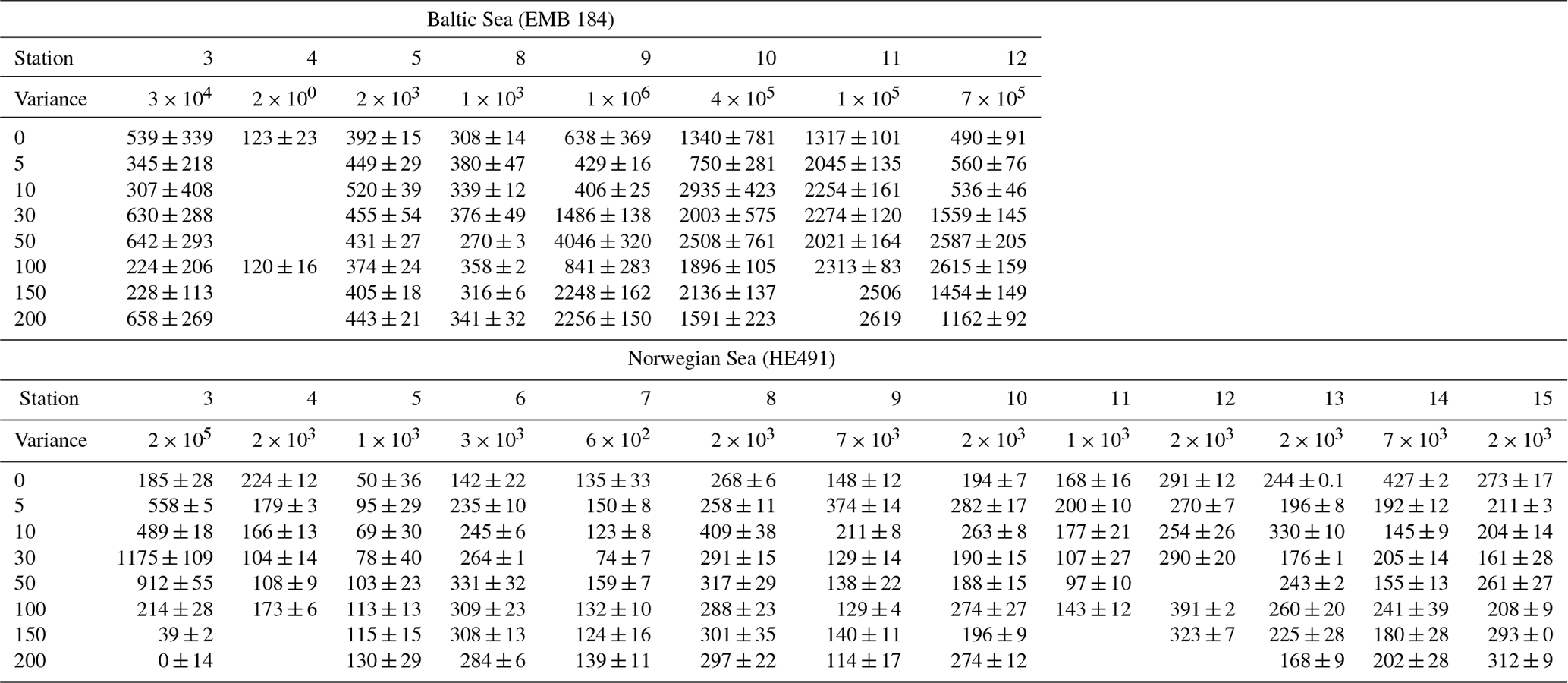
TEP concentrations at various depths (in metres) are shown in Table 3. Variance between concentrations is used to express the relative homogeneity of the parameter within the upper 2 m and results are given in units squared. During the Baltic cruise, there was a distinct change in TEP distribution between the first and second halves of the cruise (Fig. 4). TEP concentrations were lower and homogenous (average variance of 8.63×10³ µg XG eq2 L−2) for stations 3–8 but became higher in concentration and heterogeneous (average variance of 6.47×10⁵ µg XG eq2 L−2) for stations 9–12. Variance of Chl a was highest at stations 9, 10 and 12 and lowest at stations 3–5, showing a positive linear correlation between average vertical concentration and homogeneity (R2=0.95, p < 0.0001, n=8): no such correlation was observed for TEPs (R2=0.29, p=0.16, n=8). The vertical profiles for microbial counts were also taken in the Baltic Sea to investigate if there was any correlation to TEP depth profiles due to the importance of the microbial loop in TEP production and consumption (Yamada et al., 2013; Busch et al., 2017). However, no correlation or direct connection could be found between TEP profiles and microbial profiles, given as TCNs and small autotroph profiles (Fig. S1 in the Supplement).
During the Norwegian cruise, the vertical distribution of TEPs varied greatly between stations with the highest variance at station 3 (open-ocean station) and the lowest variance at stations 5, 7 and 11 (fjord/nearshore). There was no relation between TEP variance and geographical location, e.g. nearshore vs. fjord systems, vs. open ocean. Additionally, no correlation was found between TEPs and turbulent kinetic energy (TKE), measured with an acoustic Doppler velocimeter (data not shown). TKE data during the Norwegian cruise are presented in Banko-Kubis et al. (2019). TEP profiles shown in Fig. 5 were chosen based on minimum, median and maximum variance, and presented as such, since no correlation could be found to any other parameter. It is important to note that station 3 had a variance nearly 24 times larger than the second highest variance (station 9). Chl a and POC showed a moderate correlation between concentration and variance (Chl a: R2=0.67, p < 0.0006, n=13; POC: R2=0.63, p < 0.0013, n=13). However, TEPs showed no similar correlation when the putative outlier variance from station 3 was excluded (R2=0.02, p=0.66, n=12). During both cruises, TEPs were found to be enriched even when POC was not, but POC was never enriched without TEPs also being enriched.
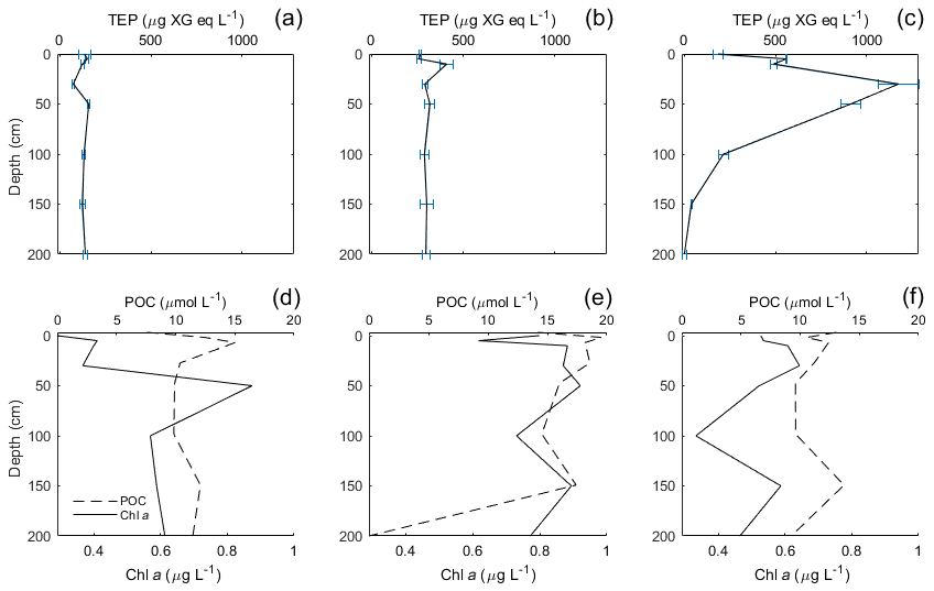
Figure 5Vertical profiles from stations 3, 7 and 12 during the Norwegian cruise, showing the vertical distribution of TEPs (a, b, c) and Chl a/POC (d, e, f). Stations were chosen based on the minimum, median and maximum vertical variance of TEPs.
TEPs are one of the main drivers for the transformation of dissolved organic matter (DOM) to particulate organic matter (POM) and its uptake into the biological pump (Mari et al., 2017). Thus, it is important to understand the vertical distribution of TEPs and what parameters drive their distribution. Previous studies focusing on vertical TEP distributions have considered depth on large scales of 5–1000 m (Ortega-Retuerta et al., 2017; Kodama et al., 2014; Cisternas-Novoa et al., 2015), and TEPs have been found to vary greatly depending on depth. Due to operational interference from research vessels and the use of large rosette water samples, most studies sample at 3–5 m for the shallowest depth and assume this surface water to be homogenous towards the surface and therefore equally representative. However, the importance and influence of the SML has been thoroughly supported (Engel et al., 2017; Cunliffe et al., 2013; Wurl et al., 2011b; Liss and Duce, 1997; Hardy, 1982), and thus there is a need to better understand the biogeochemical cycling occurring in the near-surface water and how they relate to organic matter transfer to deeper water masses. This study is the first to take a higher-resolution look at the vertical distribution of TEPs and other related parameters in the upper 2 m of the ocean. Our results show that the variability of multiple parameters can be high within the near-surface water, due to a complex biochemical system, and can occur on much smaller depth scales than previously assumed.
Table 2Enrichment factors for each station. EF ≥1 shows enrichment in the SML. NA – not available.

4.1 Relation between Chl a and TEP enrichment
Comparing the enrichment of the SML between each region showed a higher variability of enrichment within each region than between the regions (Table 2), supporting the notion that SML enrichments are a global phenomenon (Wurl et al., 2011b). Interestingly, while there was a significant but weak correlation between Chl a and TEP concentration in both the ULW and SML (ULW: R2=0.32, p < 0.0007, n=30; SML: R2=0.36, p < 0.0005, n=30), there was no significant correlation between the enrichment of TEPs and enrichment of Chl a (R2=0.045, p=0.27, n=30). This suggests that, while phytoplankton are the main source for TEP production, the transport mechanisms for TEPs and phytoplankton differ. This is in large part due to the motility of phytoplankton species, which are known to have vertical migration patterns (Bollens et al., 2010; Schuech and Menden-Deuer, 2014) and can have motility responses to physical changes like turbulence (Sengupta et al., 2017).
While the highest abundances of TEPs were found in the Baltic Sea and the lowest abundances in Cabo Verde (Fig. 2d), the highest enrichment factors were found in Cabo Verde (Fig. 2c). As the nearshore Cabo Verde waters are oligotrophic, this complements previous studies by Wurl et al. (2011a, b), which found the highest enrichment of surfactants to be in oligotrophic waters compared to mesotrophic and eutrophic. While manual sampling techniques were employed in Cabo Verde in comparison to rotating glass disc samples in the other campaigns, earlier comparative studies by Shinki et al. (2012) found both methods to collect similar SML thickness and associated biochemical parameters. Since our catamaran was modelled after Shinki et al. (2012), we are able to compare the results from both versions of the glass plate method.
Table 3TEP concentration (µg XG eq L−1) at various depths (in metres), providing an indication of the vertical distribution; variance between TEP concentrations at all depths is shown as an indicator for homogeneity (µg XG eq2 L−2).
4.2 Effect of wind speed on TEP enrichment
We observed enrichment of all parameters irrespective of either instantaneous wind speeds (2 h average) or wind speed history (24 h average), including higher wind speeds > 7 m s−1. This supports previous studies which found enrichment of material even at wind speeds > 8 m s−1 (Reinthaler et al., 2008; Kuznetsova et al., 2004), including the enrichment of TEPs in the SML at moderate wind speeds (Wurl et al., 2009). Breaking waves from moderate wind regimes can create bubble plumes in the near-surface water (Deane and Stokes, 2002; Blanchard and Woodcock, 1957), and this bubbling has proven to be an effective transport mechanism for TEPs and DOM (Robinson et al., 2019a; Zhou et al., 1998) to the SML. Thus, bubbling and turbulence at moderate wind speeds can induce more complex enrichment processes and subdue any direct correlation with wind speed. We never observed wind speeds greater than 8 m s−1, which has been found to be the threshold speed for the breakup of TEPs during experiments in a wind-wave tunnel by Sun et al. (2018). Thus, the moderate wind speeds we observed likely had an indirect positive effect on enrichment.
4.3 Effect of PP on TEP enrichment
While TEP concentrations mimic Chl a or PP due to the large contribution phytoplankton play in TEP creation (Passow, 2002a; Ortega-Retuerta et al., 2017), the enrichment of TEPs is driven by many other processes. Wurl et al. (2011a) found TEP enrichment to be irrespective of PP or negatively related with highest enrichment in oligotrophic waters with the lowest PP. Considering the relationship of PP and TEP enrichment within each region, we found this to be true for the Baltic Sea but not for the Norwegian Sea. In the Baltic Sea, as PP increased, enrichment of TEPs decreased, due to a larger increase of TEP concentration in the ULW caused from a post-bloom state (Fig. 3). However, in the Norwegian Sea, TEP enrichment matched PP, most likely due to the changing water bodies in that study, whereas the same body of water was sampled over time for the Baltic Sea and offshore Cabo Verde. While we do not have PP data for Cabo Verde, considering the positive relationship between PP and Chl a concentration in the SML for the Baltic and Norway data, Chl a concentration in the SML can be used here as proxy for PP in Cabo Verde. Under this premise, Chl a in Cabo Verde SML was similar to the Baltic in that, while Chl a and TEP SML concentrations were correlated (R2=0.68, p < 0.012, n=8), enrichment was not (R2=0.19, p=0.24, n=8).
Table 4Regional comparison of TEP, Chl a and POC enrichment and concentrations. * p < 0.05 analysed using ANOVA Tukey statistical test (95 % confidence interval). POC data from the Baltic Sea were excluded due to low n values.

p < 0.05*. p < 0.01. p < 0.001.
The oligotrophic waters of Cabo Verde present an interesting scenario for TEP production. We found the highest enrichment of TEPs in the SML here, while simultaneously observing the lowest concentrations of both Chl a and TEPs. We suggest that this is due to the abundance of precursor material as well as the increased formation of TEPs via the abiotic pathway. A tank experiment with the same setup as used by Robinson et al. (2019a), with different techniques to bubble the water, was also employed in Cabo Verde, using water from the same nearshore area as field samples. The tank was made of 10 mm polyvinyl chloride (PVC) plates in a size of 120 cm length ×110 cm width ×100 cm height. The tank had a volume of 1400 L with a 500 L aerosol chamber on top. Materials in contact with seawater were made from teflon, including liners for the wall using teflon bags. The unfiltered seawater was bubbled using the waterfall technique (Cipriano and Blanchard, 1981; Haines and Johnson, 1995) and via bubbling, large abundances of TEPs were created (Fig. S2). This suggests that, while TEP concentration in the nearshore water was low, the colloidal and precursor material for TEPs was present and only required sufficient formation mechanisms to form aggregates in the size range to be identified as TEPs. Such precursor material may have been deposited from the atmosphere; Cabo Verde is known for its Saharan dust deposition events and indeed dust events were observed during our campaign (supporting data will be shown in this special issue). This dust deposition has been shown to increase the abiotic formation of TEPs (Louis et al., 2017) and is potentially a large contributing factor to higher enrichment of TEPs in Cabo Verde. If true, this presents interesting implications for the residence time of dust which ends up floating in the SML with sufficient time for photochemical processing.
In contrast, in mesotrophic and eutrophic water, there is more biological activity present in the ULW which can increase the complexity of the system by which TEPs and their precursor material is recycled or altered before it can reach the SML. Such increase in biologically derived complexity can be seen in the depth profile data from the Baltic Sea, which showed increased heterogeneous mixing of TEPs in the water when PP was higher during the second half of the cruise. Indeed, the HSV data for all parameters show that the vertical flux processes are not straightforward to interpret.
4.4 Downward and upward fluxes of TEPs
Previous studies have found chemical characteristics to be heterogeneous in the upper 1–2 m (Goering and Wallen, 1967; Manzi et al., 1977; Momzikoff et al., 2004), substantiating the notion that vertical flux processes are too complex and strong to assume homogenous mixing. Additionally, phytoplankton communities and abundance have also been found to be heterogeneous in the water column (Cheriton et al., 2009; Dekshenieks et al., 2001; Mitchell et al., 2008). Considering the importance of ULW concentrations in estimating enrichment, the presumption of ULW as homogenous becomes problematic. When considering a parameter like TEPs which bridges the boundary of biological and chemical parameters and is so fundamentally affected by both, these studies become even more crucial indicators for the likelihood of TEP distributions to be heterogeneous, at least in surface water.
Vertical profiles were sampled for the Baltic and Norwegian seas, and in both regions, the vertical distribution of TEPs, Chl a, POC, PON were found to change from station to station. In the Baltic Sea, the vertical variance of TEPs appears to be linked to PP and the creation of TEPs from the biotic pathway. Higher deviation was seen in the second half when TEP and Chl a abundances were higher. One possible biological cause for this heterogeneous mixing could come from its link to phytoplankton. For example, Nielsen et al. (1990), Bjørnsen and Nielsen (1991) and Carpenter et al. (1995) found vertical phytoplankton patches within the water column in the open North Sea and Baltic Sea. Additionally, Cheriton et al. (2009) found that vertical oscillations cause stratification of phytoplankton into thin vertical patches. Thus, if these same processes were to occur in the near-surface environment, stratification of plankton could result in TEP precursor material being released in patches and, with rapid aggregation, create heterogeneous distribution of TEPs. This holds true especially with the majority of TEPs produced by diatoms, which are non-mobile phytoplankton that would be more susceptible to grouping and patchiness by physical forcing. This is hinted at by the heterogeneous mixing of Chl a observed during both cruises (Figs. 4 and 5), which always showed heterogeneous mixing. However, this cannot be the only mechanism, as the peak TEP concentration was not always seen at the same depth as Chl a. Further studies on vertical phytoplankton distribution in the near-surface (> 2 m) environment are needed in order to substantiate the role their patching might have on DOM and TEPs. Furthermore, there was a significant correlation between high variance of Chl a and high variance of TEPs in the Baltic Sea (R2=0.65, p < 0.028, n=7; station 4 excluded) but no correlation in the Norwegian Sea (R2=0.00, p=0.92, n=13). This suggests that with sufficient phytoplankton abundances, and reduced influence from the open ocean, the biological influences on TEP heterogeneity can dominate.
While biological sources are likely to determine the chemical characteristic of TEPs, they are not the only influence. TEPs are operationally defined polymers of acidic polysaccharides and naturally positively buoyant with highly surface active properties (Zhou et al., 1998). When unballasted by detritus or other organic matter, TEPs have a positive buoyancy and can rise to the surface at rates of 0.1–1 m d−1 (Azetsu-Scott and Passow, 2004). However, TEPs are never unattached from some type of OM, and it is this OM which helps to determine the sinking velocity of TEPs (Passow, 2002a). Additionally, the density of TEPs is dependent on the formation of its precursor material; e.g. the resulting density, and therefore sinking or rising velocity of TEPs produced from diatoms vs. bacteria will differ as well as TEPs produced from nutrient depletion vs. temperature stress (Mari et al., 2017). In near-surface water, where the ambient density of water is stratified, this could result in the immobilization of TEPs into layers of water with equal density. Thus, heterogeneous mixing of TEPs may be caused by a sort of vertical filtering via TEP density and surrounding water density.
The vertical profiles for TEPs, Chl a and POC during the Norwegian cruise showed no correlation with any of the sea state parameters. The same was true during the Baltic cruise, which had matching increases in TEP and Chl a concentrations but differing depth profiles (Fig. 4). On seasonal scales, TEPs have been shown to match Chl a and POC trends (Wurl et al., 2011a; Ortega-Retuerta et al., 2017; Mari et al., 2017; Zamanillo et al., 2019) supporting the notion of phytoplankton blooms as a main source for TEP production in the ocean and subsequently TEPs as a main source of POC uptake. This is corroborated in our data. However, when considering the vertical transport of these substances, this relationship is broken or interrupted by the influence of additional mechanisms. Due to the lack of direct correlation between any one parameter and TEP concentration or enrichment, we suggest that the vertical flux mechanisms of TEPs in the near-surface environment are complex. Any positive effects on enrichment, such as wind speed and bubble formation, are only partially responsible. However, with the consistent changing of vertical profiles of TEPs, it is clear that these complex fluxes can often result in heterogeneous layering of TEPs within the upper 2 m of the ocean. Indeed within a few centimetres, TEP concentration can change by up to 291 %, with no parameter acting as a proxy to suggest homogeneity or heterogeneity. Therefore, it is important for future studies to accommodate this uncertainty of ULW values and for a standardized depth for all ULW to be incorporated.
Data have been submitted to PANGAEA database: https://doi.pangaea.de/10.1594/PANGAEA.903834 (Robinson et al., 2019b).
The supplement related to this article is available online at: https://doi.org/10.5194/os-15-1653-2019-supplement.
All authors have substantially contributed to the manuscript with their involvement in the research cruises, the collection of data, analysis of the data or contribution to the writing and discussion of the manuscript.
The authors declare that they have no conflict of interest.
This article is part of the special issue “Marine organic matter: from biological production in the ocean to organic aerosol particles and marine clouds (ACP/OS inter-journal SI)”. It is not associated with a conference.
This study received funding from the Leibniz Society (MarParCloud, SAW-2016_TROPOS-2). We greatly appreciate technical assistance by the crews from both the R/V Heinke and R/V Elisabeth Mann Borgese during the research cruises. Further, we would like to thank the MarParCloud group for collaborative efforts during the Cabo Verde campaign, especially Manuela van Pinxteren, Nadja Triesch and Khanneh Wadinga Fomba for coordination efforts. From the University of Oldenburg, we would like to thank Maren Striebel and Hanna Banko-Kubis for help sampling during the Norwegian cruise and Heike Rickels for nutrient analysis. From the Leibniz Institute for Baltic Sea Research, we would like to thank Christian Burmeister for Chl a measurements, Jenny Jeschek for POC analysis and Katja Kaeding for flow cytometry measurements.
This research has been supported by the Leibniz Society (grant no. SAW-2016_TROPOS-2).
This paper was edited by Mario Hoppema and reviewed by two anonymous referees.
Azetsu-Scott, K. and Passow, U.: Ascending marine particles: Significance of transparent exopolymer particles (TEP) in the upper ocean, Limnol. Oceanogr., 49, 741–748, https://doi.org/10.4319/lo.2004.49.3.0741, 2004.
Banko-Kubis, H. M., Wurl, O., Mustaffa, N. I. H., and Ribas-Ribas, M.: Gas transfer velocities in norwegian fjords and the adjacent north atlantic waters, Oceanologia, 61, 460–470, https://doi.org/10.1016/j.oceano.2019.04.002, 2019.
Behrenfeld, M. J. and Falkowski, P. G.: A consumer's guide to phytoplankton primary productivity models, Limnol. Oceanogr., 42, 1479–1491, https://doi.org/10.4319/lo.1997.42.7.1479, 1997.
Bittar, T. B., Passow, U., Hamaraty, L., Bidle, K. D., and Harvey, E. L.: An updated method for the calibration of transparent exopolymer particle measurements, Limnol. Oceanogr.-Methods, 16, 621–628, https://doi.org/10.1002/lom3.10268, 2018.
Bjørnsen, P. K. and Nielsen, T. G.: Decimeter scale heterogeneity in the plankton during a pycnocline bloom of Gyrodinium aureolum, Mar. Ecol. Prog. Ser., 73, 263–267, https://doi.org/10.3354/meps073263 1991.
Blanchard, D. C. and Woodcock, A. H.: Bubble Formation and Modification in the Sea and its Meteorological Significance, Tellus, 9, 145–158, https://doi.org/10.3402/tellusa.v9i2.9094, 1957.
Bollens, S. M., Rollwagen-Bollens, G., Quenette, J. A., and Bochdansky, A. B.: Cascading migrations and implications for vertical fluxes in pelagic ecosystems, J. Plankton Res., 33, 349–355, https://doi.org/10.1093/plankt/fbq152, 2010.
Busch, K., Endres, S., Iversen, M. H., Michels, J., Nöthig, E.-M., and Engel, A.: Bacterial Colonization and Vertical Distribution of Marine Gel Particles (TEP and CSP) in the Arctic Fram Strait, Frontiers in Marine Science, 4, 166, https://doi.org/10.3389/fmars.2017.00166, 2017.
Carpenter, E. J., Janson, S., Boje, R., Pollehne, F., and Chang, J.: The dinoflagellate Dinophysis norvegica: biological and ecological observations in the Baltic Sea, Eur. J. Phycol., 30, 1–9, https://doi.org/10.1080/09670269500650751, 1995.
Cheriton, O., McManus, M., Stacey, M., and Steinbuck, J.: Physical and biological controls on the maintenance and dissipation of a thin phytoplankton layer, Mar. Ecol. Prog. Ser., 378, 55–69, https://doi.org/10.3354/meps07847, 2009.
Cipriano, R. J. and Blanchard, D. C.: Bubble and aerosol spectra produced by a laboratory “breaking wave”, J. Geophys. Res.-Oceans, 86, 8085–8092, https://doi.org/10.1029/jc086ic09p08085, 1981.
Cisternas-Novoa, C., Lee, C., and Engel, A.: Transparent exopolymer particles (TEP) and Coomassie stainable particles (CSP): Differences between their origin and vertical distributions in the ocean, Mar. Chem., 175, 56–71, https://doi.org/10.1016/j.marchem.2015.03.009, 2015.
Cunliffe, M. and Murrell, C.: The sea-surface microlayer is a gelatinous biofilm, ISME J., 3, 1001–1003, https://doi.org/10.1038/ismej.2009.69, 2009.
Cunliffe, M. and Wurl, O.: Guide to the best practices to study the ocean's surface, Marine Biological Association of the United Kingdom, Plymouth, UK, 118 pp., 2014.
Cunliffe, M., Engel, A., Frka, S., Gasparovic, B., Guitart, C., Murrell, C., Salter, M., Stolle, C., Upstill-Goddard, R., and Wurl, O.: Sea surface microlayers: A unified physicochemical and biological perspective of the air–ocean interface, Prog. Oceanogr., 109, 104–116, https://doi.org/10.1016/j.pocean.2012.08.004, 2013.
Deane, G. and Stokes, M.: Scale dependence of bubble creation mechanisms in breaking waves, Nature, 418, 839–844, https://doi.org/10.1038/nature00967, 2002.
Dekshenieks, M. M., Donaghay, P. L., Sullivan, J. M., Rines, J. E., Osborn, T. R., and Twardowski, M. S.: Temporal and spatial occurrence of thin phytoplankton layers in relation to physical processes, Mar. Ecol. Prog. Ser., 223, 61–71, https://doi.org/10.3354/meps223061 2001.
Engel, A.: Distribution of transparent exopolymer particles (TEP) in the northeast Atlantic Ocean and their potential significance for aggregation processes, Deep-Sea Res. Pt. I, 51, 83–92, https://doi.org/10.1016/j.dsr.2003.09.001, 2004.
Engel, A., Bange, H. W., Cunliffe, M., Burrows, S. M., Friedrichs, G., Galgani, L., Herrmann, H., Hertkorn, N., Johnson, M., and Liss, P. S.: The ocean's vital skin: Toward an integrated understanding of the sea surface microlayer, Frontiers in Marine Science, 4, 165, https://doi.org/10.3389/fmars.2017.00165, 2017.
Goering, J. J. and Wallen, D.: The vertical distribution of phosphate and nitrite in the upper one-half meter of the Southeast Pacific Ocean, Deep-Sea Res., 14, 29–33, 1967.
Grasshoff, K., Kremling, K., and Ehrhardt, M.: Methods of seawater analysis, Wiley, New York, https://doi.org/10.1002/9783527613984, 1999.
Haines, M. A. and Johnson, B. D.: Injected bubble populations in seawater and fresh water measured by a photographic method, J. Geophys. Res., 100, 7057–7068, https://doi.org/10.1029/94jc03226, 1995.
Hardy, J. T.: The Sea Surface Microlayer: Biology, Chemistry and Anthropogenic Enrichment, Prog. Oceanogr., 11, 307–328, https://doi.org/10.1016/0079-6611(82)90001-5, 1982.
Harvey, G. and Burzell, L.: A Simple Microlayer Method for Small Samples, Limnol. Oceanogr., 17, 156–157, https://doi.org/10.4319/lo.1972.17.1.0156, 1972.
Kodama, T., Kurogi, H., and Okazaki, M.: Vertical distribution of transparent exopolymer particle (TEP) concentration in the oligotrophic western tropical North Pacific, Mar. Ecol. Prog. Ser., 513, 29–37, https://doi.org/10.3354/meps10954, 2014.
Kuznetsova, M., Lee, C., Aller, J., and Frew, N.: Enrichment of amino acids in the sea surface microlayer at coastal and open ocean sites in the North Atlantic Ocean, Limnol. Oceanogr., 49, 1605–1619, https://doi.org/10.4319/lo.2004.49.5.1605 2004.
Liss, P. and Duce, R.: The Sea Surface and Global Change, Cambridge University Press, 251–286, 1997.
Liss, P. S., Liss, P. S., and Duce, R. A.: The sea surface and global change, Cambridge University Press, 251–286, 2005.
Louis, J., Pedrotti, M. L., Gazeau, F., and Guieu, C.: Experimental evidence of formation of Transparent Exopolymer Particles (TEP) and POC export provoked by dust addition under current and high pCO2 conditions, PloS one, 12, e0171980, https://doi.org/10.1371/journal.pone.0171980, 2017.
Manzi, J., Stofan, P., and Dupuy, J.: Spatial heterogeneity of phytoplankton populations in estuarine surface microlayers, Mar. Biol., 41, 29–38, https://doi.org/10.1007/bf00390578, 1977.
Mari, X., Passow, U., Migon, C., Burd, A. B., and Legendre, L.: Transparent exopolymer particles: Effects on carbon cycling in the ocean, Prog. Oceanogr., 151, 13–37, https://doi.org/10.1016/j.pocean.2016.11.002, 2017.
Marie, D., Simon, N., Guillou, L., Partensky, F., and Vaulot, D.: Flow cytometry analysis of marine picoplankton, in: In Living Color, 421–454, Springer, Berlin, Heidelberg, 2000.
Mitchell, J. G., Yamazaki, H., Seuront, L., Wolk, F., and Li, H.: Phytoplankton patch patterns: seascape anatomy in a turbulent ocean, J. Marine Syst., 69, 247–253, https://doi.org/10.1016/j.jmarsys.2006.01.019, 2008.
Momzikoff, A., Brinis, A., Dallot, S., Gondry, G., Saliot, A., and Lebaron, P.: Field study of the chemical characterization of the upper ocean surface using various samplers, Limnol. Oceanogr.-Meth., 2, 374–386, https://doi.org/10.4319/lom.2004.2.374, 2004.
Nielsen, T. G., Kiørboe, T., and Bjørnsen, P. K.: Effects of a Chrysochromulina polylepis subsurface bloom on the planktonic community, Mar. Ecol. Prog. Ser., 62, 21–35, https://doi.org/10.3354/meps062021 1990.
Ortega-Retuerta, E., Sala, M. M., Borrull, E., Mestre, M., Aparicio, F. L., Gallisai, R., Antequera, C., Marrasé, C., Peters, F., and Simó, R.: Horizontal and Vertical Distributions of Transparent Exopolymer Particles (TEP) in the NW Mediterranean Sea Are Linked to Chlorophyll a and O2 Variability, Front. Microbiol., 7, 2159, https://doi.org/10.3389/fmicb.2016.02159, 2017.
Passow, U.: Production of transparent exopolymer particles (TEP) by phyto- and bacterioplankton, Mar. Ecol. Prog. Ser., 236, 1–12, https://doi.org/10.3354/meps236001, 2002a.
Passow, U.: Transparent exopolymer particles (TEP) in aquatic environments, Prog. Oceanogr., 55, 287–333, https://doi.org/10.1038/npre.2007.1182.1, 2002b.
Passow, U. and Alldredge, A.: A dye-binding assay for the spectrophotometric measurement of transparent exopolymer particles (TEP), Limnol. Oceanogr., 40, 1326–1335, https://doi.org/10.4319/lo.1995.40.7.1326, 1995.
Reinthaler, T., Sintes, E., and Herndl, G.: Dissolved organic matter and bacterial production and respiration in the sea–surface microlayer of the open Atlantic and the western Mediterranean Sea, Limnol. Oceanogr., 53, 122–136, https://doi.org/10.4319/lo.2008.53.1.0122, 2008.
Ribas-Ribas, M., Hamizah Mustaffa, N. I., Rahlff, J., Stolle, C., and Wurl, O.: Sea Surface Scanner (S3): A Catamaran for High-Resolution Measurements of Biogeochemical Properties of the Sea Surface Microlayer, J. Atmos. Ocean. Tech., 34, 1433–1448, https://doi.org/10.1175/jtech-d-17-0017.1, 2017.
Robinson, T.-B., Wurl, O., Bahlmann, E., Jürgens, K., and Stolle, C.: Rising bubbles enhance the gelatinous nature of the air–sea interface, Limnol. Oceanogr., 64, 2358–2372, https://doi.org/10.1002/lno.11188, 2019a.
Robinson, T.-B., Stolle, C., and Wurl, O.: Biochemical parameters in the underlying water (ULW) from Cape Verde, the Baltic Sea, and Norwegian fjords/Sea, PANGAEA, https://doi.org/10.1594/PANGAEA.903834 (dataset in review), 2019b.
Schuech, R. and Menden-Deuer, S.: Going ballistic in the plankton: anisotropic swimming behavior of marine protists, Limnol. Oceanogr., 4, 1–16, https://doi.org/10.1215/21573689-2647998, 2014.
Sengupta, A., Carrara, F., and Stocker, R.: Phytoplankton can actively diversify their migration strategy in response to turbulent cues, Nature, 543, 1–42, https://doi.org/10.1038/nature21415, 2017.
Shinki, M., Wendeberg, M., Vagle, S., Cullen, J. T., and Hore, D. K.: Characterization of adsorbed microlayer thickness on an oceanic glass plate sampler, Limnol. Oceanogr.-Meth., 10, 728–735, 10.4319/lom.2012.10.728, 2012.
Sieburth, J.: Microbiological and organic-chemical processes in the surface and mixed layers, in: Air-Sea Exchange of Gases and Particles, edited by: Liss, P. and Slinn, W., Reidel Publishers Co, Hingham, MA, 121–172, 1983.
Sun, C.-C., Sperling, M., and Engel, A.: Effect of wind speed on the size distribution of gel particles in the sea surface microlayer: insights from a wind-wave channel experiment, Biogeosciences, 15, 3577–3589, https://doi.org/10.5194/bg-15-3577-2018, 2018.
Wasmund, N., Topp, I., and Schories, D.: Optimising the storage and extraction of chlorophyll samples, Oceanologia, 48, 125–144, 2006.
Wetzel, R. G. and Likens, G.: Limnological Analyses, Springer New York, 85–112, 2000.
Wurl, O. and Holmes, M.: The gelatinous nature of the sea-surface microlayer, Mar. Chem., 110, 89–97, https://doi.org/10.1016/j.marchem.2008.02.009, 2008.
Wurl, O., Miller, L., Röttgers, R., and Vagle, S.: The distribution and fate of surface-active substances in the sea-surface microlayer and water column, Mar. Chem., 115, 1–9, https://doi.org/10.1016/j.marchem.2009.04.007, 2009.
Wurl, O., Miller, L., and Vagle, S.: Production and fate of transparent exopolymer particles in the ocean, J. Geophys. Res., 116, C00H13, https://doi.org/10.1029/2011JC007342, 2011a.
Wurl, O., Wurl, E., Miller, L., Johnson, K., and Vagle, S.: Formation and global distribution of sea-surface microlayers, Biogeosciences, 8, 121–135, https://doi.org/10.5194/bg-8-121-2011, 2011b.
Wurl, O., Stolle, C., Van Thuoc, C., The Thu, P., and Mari, X.: Biofilm-like properties of the sea surface and predicted effects on air–sea CO2 exchange, Prog. Oceanogr., 144, 15–24, https://doi.org/10.1016/j.pocean.2016.03.002, 2016.
Wurl, O., Ekau, W., Landing, W. M., and Zappa, C. J.: Sea surface microlayer in a changing ocean–A perspective, Elem. Sci. Anth., 5, 31, https://doi.org/10.1525/elementa.228, 2017.
Yamada, Y., Fukuda, H., Inoue, K., Kogure, K., and Nagata, T.: Effects of attached bacteria on organic aggregate settling velocity in seawater, Aquat. Microb. Ecol., 70, 261–272, https://doi.org/10.3354/ame01658, 2013.
Yamada, Y., Yokokawa, T., Uchimiya, M., Nishino, S., Fukuda, H., Ogawa, H., and Nagata, T.: Transparent exopolymer particles (TEP) in the deep ocean: full-depth distribution patterns and contribution to the organic carbon pool, Mar. Ecol. Prog. Ser., 583, 81–93, https://doi.org/10.3354/meps12339, 2017.
Zamanillo, M., Ortega-Retuerta, E., Nunes, S., Rodríguez-Ros, P., Dall'Osto, M., Estrada, M., Montserrat Sala, M., and Simó, R.: Main drivers of transparent exopolymer particle distribution across the surface Atlantic Ocean, Biogeosciences, 16, 733–749, https://doi.org/10.5194/bg-16-733-2019, 2019.
Zhou, J., Mopper, K., and Passow, U.: The role of surface-active carbohydrates in the formation of transparent exopolymer particles by bubble adsorption of seawater, Limnol. Oceanogr., 43, 1860–1871, https://doi.org/10.4319/lo.1998.43.8.1860, 1998.