the Creative Commons Attribution 4.0 License.
the Creative Commons Attribution 4.0 License.
 | 16 Dec 2019
Influence of the summer deep-sea circulations on passive drifts among the submarine canyons in the northwestern Mediterranean Sea
Morane Clavel-Henry
Jordi Solé
Miguel-Ángel Ahumada-Sempoal
Nixon Bahamon
Florence Briton
Guiomar Rotllant
Joan B. Company
Marine biophysical models can be used to explore the displacement of individuals in and between submarine canyons. Mostly, the studies focus on the shallow hydrodynamics in or around a single canyon. In the northwestern Mediterranean Sea, knowledge of the deep-sea circulation and its spatial variability in three contiguous submarine canyons is limited. We used a Lagrangian framework with three-dimensional velocity fields from two versions of the Regional Ocean Modeling System (ROMS) to study the deep-bottom connectivity between submarine canyons and to compare their influence on the particle transport. From a biological point of view, the particles represented eggs and larvae spawned by the deep-sea commercial shrimp Aristeus antennatus along the continental slope in summer. The passive particles mainly followed a southwest drift along the continental slope and drifted less than 200 km considering a pelagic larval duration (PLD) of 31 d. Two of the submarine canyons were connected by more than 27 % of particles if they were released at sea bottom depths above 600 m. The vertical advection of particles depended on the depth where particles were released and the circulation influenced by the morphology of each submarine canyon. Therefore, the impact of contiguous submarine canyons on particle transport should be studied on a case-by-case basis and not be generalized. Because the flows were strongly influenced by the bottom topography, the hydrodynamic model with finer bathymetric resolution data, a less smoothed bottom topography, and finer sigma-layer resolution near the bottom should give more accurate simulations of near-bottom passive drift. Those results propose that the physical model parameterization and discretization have to be considered for improving connectivity studies of deep-sea species.
- Article
(3212 KB) -
Supplement
(529 KB) - BibTeX
- EndNote


Lagrangian particles coupled with three-dimensional hydrodynamic models are useful to assess the impact of ocean circulation on the drift of small elements or individuals. It allows for the exploration of various scenarios of dispersal and increases knowledge in several fields of marine systems, such as predicting the direction of oil spills (Jones et al., 2016); understanding the circulation of microplastics (Lebreton et al., 2012); estimating the impact of aquaculture (Cromey and Black, 2005); and describing the spatial dispersion of crustaceans, fish, and other marine larvae (Ahumada-Sempoal et al., 2015; North, 2008; Ospina-Aìlvarez et al., 2013). Particles in the open ocean are susceptible to advection between locations, influenced by regional currents and mesoscale features such as eddies and meanders (Ahumada-Sempoal et al., 2013). The particles without implemented behavior are called passive and are efficiently used to study the inactive transport of elements. They also provide a useful approximation of larval drifts when the ecological knowledge on the early life cycle is scarce. The individual-based models (IBM) configure each Lagrangian particle with characteristics parameterized by the modeler. In marine ecological studies, IBMs provide a representation of the potential connectivity between geographically separated subpopulations, with implications for fishery management and conservation plans (Andrello et al., 2013; Basterretxea et al., 2012; Kough et al., 2013; Siegel et al., 2003).
Simulation of marine passive drifts provides a picture of the highly dynamic circulation in the vicinity of the submarine canyons. Influence of canyons on the transport of particles and living organisms has begun to raise interest, but only a few studies are dealing with the Lagrangian transport of particles specifically in those small-scale topographic structures (Ahumada-Sempoal et al., 2015; Kool et al., 2015; Shan et al., 2014). In the northwestern (NW) Mediterranean Sea, several submarine canyons, whose heads are incising the continental shelf (i.e., Cap de Creus, Palamós, and Blanes canyons), generate mesoscale features from the main circulation pattern (Millot, 1999) called the Northern Current (NC). When the NC crosses a canyon, it causes a downwelling on the upstream wall and an upwelling on the downstream wall in the 100–200 m layer depth (Ahumada-Sempoal et al., 2015; Jordi et al., 2006), or it causes the opposite at lower depths (Flexas et al., 2008). Within the canyons, near-bottom currents produce a closed circulation (Palanques et al., 2005; Solé et al., 2016), which loses strength with the depth (Flexas et al., 2008; Granata et al., 1999). The canyon shape enhances the downwelling of water and its components (sediment and organic carbon; Puig et al., 2003, biogenic or inorganic particles; Granata et al., 1999), and it provides favorable and diverse habitats for benthic species (Fernandez-Arcaya et al., 2017). Those exchanges proceed at different velocity rates following the condition of the waters. For example, cascading of winter water masses drives suspended substances along the funnel structure of the canyons (Canals et al., 2009). In summer, the stratification of the water column is well-established in the NW Mediterranean Sea decoupling the mixed layer from the rest of the water column (Rojas et al., 1995) and slowing the downward sink of biogenic particles (Granata et al., 1999). During that season, the circulation of the NC is shallower (250 m deep), wider (50 km wide) and less intense than in winter (Millot, 1999).
To date, the impact of the circulation on the dispersal of particles was estimated with hydrophysical data (Ahumada-Sempoal et al., 2015; Granata et al., 1999; Rojas et al., 1995) and with sediment traps (Durrieu de Madron et al., 1999; Lopez-Fernandez et al., 2013) in shallow waters above the NW Mediterranean submarine canyons. None of the previous studies simulated the particle transport at a deeper layer or showed the particle exchanges among different water layers of submarine canyons. Information on the roles of the upper part of the canyon on both horizontal and vertical transport of particles is not clear (e.g., 0–300 m; Granata et al., 1999), and for deeper parts this information is rarely provided. In accordance with those facts, we questioned if the deep-sea circulation mechanism in each submarine canyons of the NW Mediterranean Sea can be generalized.
In this study, deep passive drifts along the NW Mediterranean continental slope are simulated to determine the influence of the summer circulation modulated by the presence of the submarine canyons. We partly focused on the drift sensitivity to deep circulation using the outputs of two hydrodynamic numerical models to approach the transport uncertainties. With this study, we are expecting to provide a first insight into the deep connectivity between submarine canyons to improve the management of their grounds, namely of the deep-sea shrimp Aristeus antennatus.
The influence of deep circulation on passive drifts among the submarine canyons of the NW Mediterranean Sea was analyzed through the dispersal of Lagrangian particles.
2.1 Hydrodynamic models
The sensitivity of dispersal to the circulation was generated with the use of two available hydrodynamic models, which covered the area of the submarine canyons in the northwestern Mediterranean Sea (see Fig. 1). Because of the parameterization related to the topography (i.e., bathymetric data sets and smoothing) and the vertical layer discretization in the two hydrodynamic models, small differences in morphology of the submarine canyons were expected to impact the flow circulation.
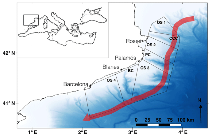
Figure 1Map of the study area. Release zones are represented along the northwestern Mediterranean Sea: open slope (OS) 1, Cap de Creus canyon (CCC), OS 2, Palamós canyon (PC), OS 3, Blanes canyon (BC), and OS 4. The red arrow indicates the direction of the Northern Current. Bathymetry was extracted from EMODnet (http://www.emodnet-bathymetry.eu, last access: December 2018).
The two hydrodynamic models were climatological simulations using the Regional Ocean Model System (ROMS; Shchepetkin and McWilliams, 2005), a free-surface terrain-following primitive equations ocean model. ROMS includes accurate and efficient physical and numerical algorithms (Shchepetkin, 2003). The two models were referred to by their implementation versions, ROMS-Rutgers and ROMS-Agrif (Debreu et al., 2012), for the sake of clarity. In the present paper, the ROMS-Rutgers configuration and its validations are presented, while ROMS-Agrif has already been used and validated in Ahumada-Sempoal et al. (2013, 2015).
The ROMS-Rutgers model was forced by a climatological atmospheric forcing. The air temperature, shortwave radiation, longwave radiation, precipitation, cloud cover, and freshwater flux used to force the model came from the ERA-40 reanalysis (Uppala et al., 2005). Surface pressure came from the ERA-Interim reanalysis (Dee et al., 2011). All these variables had a spatial resolution of 1∘ and a time resolution of 6 h. QuikSCAT blend data were used for wind forcing (both zonal and meridional). The wind had a spatial resolution of 0.25∘ and a time resolution of 6 h. The boundary conditions were obtained from NEMO (available from https://www.nemo-ocean.eu/, last access: March 2012; these simulations were reported in Adani et al., 2011) and interpolated to the ROMS grid to define a sponge layer of 10 horizontal grid points with a nudging relaxation time of 30 d. This methodology for the implementation of the model in the area followed the same procedure as the one already tested in the Alboran Sea (Solé et al., 2016). This model implementation was already used in previous publications as a hydrodynamic model coupled with a fisheries model (Coll et al., 2016).
The simulation domain ranges from 0.65∘ W to 6.08∘ E and from 38 to 43.69∘ N. The grid resolution is 2 km (with 256×384 grid points horizontally) and the vertical domain is discretized using 40 vertical levels with a finer resolution near the surface (S coordinate surface and bottom parameter are θs=5 and θb=0.4). Thus, the thickness of the near-bottom layer on the continental slopes delimited by the 500 and 800 m isobaths is 24 m (±3.2 m). The advection scheme used in our simulations was MPDATA (recursive flux-corrected 3-D advection of particles; Smolarkiewicz and Margolin, 1998) and Large–McWilliams–Doney (LMD) mixing as a subgrid-scale turbulent mixing closure scheme (Large et al., 1994), also known as the K-Profile Parameterization (KPP) scheme. The air–sea interaction used for the boundary layer in ROMS was based on the bulk parameterization (Fairall et al., 1996). Bathymetry grid with a horizontal resolution of 100 m was provided by the Geoscience department of the Institute of Marine Sciences (ICM-CSIC, Barcelona) and fitted to the grid of the model. We ran the ROMS-Rutgers model version 3.6 using climatological atmospheric forcing and boundary conditions. The initial conditions to start the simulations were obtained using the same interpolated fields as the ones used for the boundary conditions for all variables. After an 8-year spin-up period with a baroclinic time step of 120 s, we used the ninth year as the study period.
The regional ROMS-Rutgers implementation has been daily saved and validated. First, we compared the simulations with the coarser model used for the initial and boundary conditions (NEMO). Second, the model was compared to the ARGO float vertical data profiles of temperature and salinity to test the correct structure of the simulated water column within the year. For the ARGO tests, we selected 1900 casts in the area from October 2003 to December 2012. The data collected cover depths from the surface down to a maximum of 720 m. The ARGO vertical profile resolution was 5 m from the surface to 200 and 25 m from 200 to 720 m. We grouped the ARGO casts by months and by six subareas dividing the domain according to the Coriolis force divided by the bottom depth (Fig. 2). Then, we selected the subareas that have more than 30 ARGO profiles for each month, we calculated a monthly averaged profile of ARGO, and we compared them with the modeled climatologic profile (monthly average).
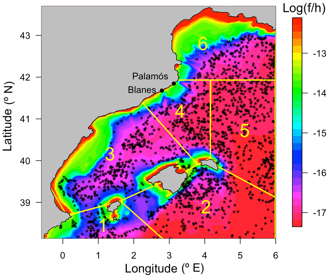
Figure 2Map of the ROMS-Rutgers model domain and position of ARGO buoys. The color bar represents the Coriolis parameter (f) divided by the depth (h) (f∕h in a zebra color palette). The six subareas selected to validate the model using ARGO float observations are shown by yellow polygons. The black dots in the domain represent all the ARGO profiles considered.
The main general behavior of the ROMS-Rutgers model simulation was coherent with the lower-resolution model (NEMO) and with the reported hydrography of the northwestern Mediterranean Sea. The model also successfully reproduced the main seasonal behavior of the different water masses. A Taylor diagram (Taylor, 2001) was used to display the correlation, root mean square error (RMSE), and standard deviation (SD) between the monthly averages of the ROMS-Rutgers model profiles and ARGO profiles by subareas (Fig. 3). The comparison showed reasonably good correlations of statistical significance. For temperature, the correlation between model and ARGO was higher than 0.7 during 10 of the 12 months, while for salinity it was higher than 0.95 for all the months. As it is shown in Fig. 3, during the month of September, the correlations in the Taylor diagram for temperature and salinity were higher than 0.9 in both variables. The month of September was selected because the thermocline in our domain disappears and the mixing process at that period of the year is likely to vary the most. Consequently, it shows that the circulation over different depths has been well reproduced in the model.
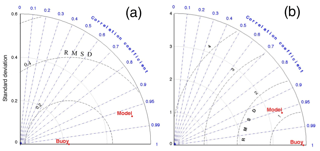
Figure 3Taylor diagrams for validation of ROMS-Rutgers. Example of comparison between buoys (ARGO floats) and ROMS-Rutgers model simulations during September. (a) The temperature of float versus model and (b) the salinity of float versus model. Radial from the origin (0, 0) are the correlation coefficients, internal circles centered on the origin are standard deviations, and internal circles centered at the buoy position are root mean square differences (RMSDs).
The second set of velocity and thermodynamic fields was provided by ROMS-Agrif, built and validated in Ahumada-Sempoal et al. (2013). The simulation domain ranges from 40.21 to 43.93∘ N and 0.03∘ W to 6∘ E. It has a finer horizontal resolution (∼1.2 km), with 32 sigma levels of a finer resolution near the surface and coarser resolution near the bottom (S coordinate surface and bottom parameters are θs=7 and θb=0) than ROMS-Rutgers. The average thickness of the near-bottom layer is 54 m and is approximately 2 times thicker than the near-bottom layer from ROMS-Rutgers. The model was one-way nested from a coarse regional resolution model of 4 km. Bathymetry was derived from the ETOPO2-arcminute model (with horizontal grid resolution of 3 km) from Smith and Sandell (1997). Surface forcing and initial and boundary conditions were built with the ROMSTOOLS package (Penven et al., 2008), running a 10-year simulation of the model.
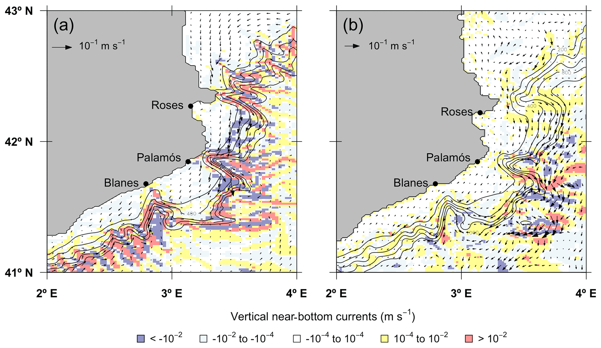
Figure 4Vertical velocity and horizontal velocity vectors at bottom in the northwestern Mediterranean Sea in the (a) ROMS-Rutgers and (b) ROMS-Agrif models. Colors from blue to red according to the downward or upward (negative or positive) vertical velocity. Continuous black lines are the isobaths adapted from the bathymetry of the hydrodynamic models.
In the ROMS-Rutgers configuration, the bottom circulation followed a southward direction along the bottom slope, except in the area south of Blanes canyon (Fig. 4). Over the bottom floor of the continental slope, the highest velocities reached 8.5 cm s−1 on the southern mouth of Palamós canyon. The fastest vertical velocities were at sea bottom deeper than 400 m and are mostly located among the submarine canyons. The minimum and maximum velocity values (−1.4 and 1.7 mm s−1, respectively) were located in Palamós canyon. In ROMS-Agrif, the hydrodynamic model had higher near-bottom currents in the areas at the north and south of Palamós canyon. The maximum velocity reached 11.6 cm s−1 off the continental slope between Palamós and Blanes canyons. Higher intensities of vertical near-bottom current were also in those areas (see Fig. 4) even though the most extreme values of vertical velocity were −1.23 and 1.11 mm s−1 on the bottom off the continental rise.
2.2 Practical study
In this study, we considered some characteristics of the deep-sea shrimp Aristeus antennatus for the initial configuration of the simulated passive drifters. A. antennatus is a benthic commercial species distributed over the area of study (Demestre and Lleonart, 1993; Sardà et al., 1997), and it is an important source of income for the fishing harbors of the NW Mediterranean Sea (Gorelli et al., 2014).
The spawning peak of A. antennatus – and release of particles – occurred in summer (July to September; Demestre and Fortuño, 1992) in the sea bottom delimited by the isobaths of 500 and 800 m, i.e., on average 650 m (Sardà et al., 1997; Tudela et al., 2003) at midnight (Schram et al., 2010). The ecology of the early pelagic stages (eggs and larvae) is hardly known due to the difficulty to catch the larvae in the open sea and to keep the adults in captivity alive.
For setting the duration of simulated drift, we used the pelagic larval duration (PLD) of the shrimp, i.e., the time a larva spends in the water column from spawning to the first post-larval stage. As individuals of the superfamily Penaeidae (which contains the species A. antennatus) release eggs in the environment before hatching (Dall, 1990), the PLD definition was extended to account for the duration of the embryonic stage. To overcome the situation of an unknown PLD for A. antennatus, we fitted a linear model to the relation between the duration of eggs developing into the post-larvae stage from 43 penaeid species by reviewing research articles (see Table S1 in the Supplement) and the temperature of the water in which the larvae were reared. The linear model, whose initial assumptions were verified (see Fig. S1) and had a coefficient of determination R2=56 %, was the following:
where T is water temperature in degrees Celsius. Then, the effect of water temperature on the duration of the larval stage had the shape of an exponential law (O'Connor et al., 2007; Pepin, 1991). When particles were at the deep-sea bottom, we could estimate their PLD to be 31 d because the seawater temperature was approximately 13.2 ∘C. The duration appeared to be shorter than the PLD for other deep-sea species (Arellano et al., 2014: Etter and Bower, 2015; Young et al., 2012) but was in agreement with PLD for temperate invertebrates (Levin and Bridges, 1995; Thatje et al., 2005; Williamson, 1982) and PLDs of penaeid species predicted in Dall (1990).
Using the passive drift simulations, we started to explore the simplest hypothesis around the larval ecology, which corresponds to the absence of larval behavior (such as egg buoyancy or swimming abilities). The drift of particles is used as a first step to approach the unknown larval cycle. The good management of the fishery has raised the interest of science to have a better knowledge of the species ecology. Last, the particles are used to estimate potential connections among the fishing grounds of A. antennatus. It contributes to complement the research made in parental genetic studies (Sardà and Company, 2012), which have shown the high dispersive capacity of A. antennatus without revealing its connectivity paths.
2.3 Biophysical model
Particle dispersal was simulated with the open-source IBM code Ichthyop (Lett et al., 2008) version 3.3, which is a free user-friendly toolset used in numerous individual dispersal studies in the western Mediterranean Sea (e.g., Ospina-Aìlvarez et al., 2013; Palmas et al., 2017). Displacements of virtual particles are computed by integrating the differential equation using a Runge–Kutta 4th order (RK4) advection scheme:
where dX is the three-dimensional displacement vector of the particles during a time step dt of 30 min under the velocity vector U from the hydrodynamic models. RK4 is a stable and reliable multistep method for numerical integration (North et al., 2009; Qiu et al., 2011) and is commonly used in Lagrangian dispersal models (North et al., 2009; Chen et al., 2003; Paris et al., 2013). The Ichthyop algorithm used trilinear and linear interpolations in space and time from the daily average ROMS velocity field output to each particle position at all time steps. Attributes (geographical coordinates and depth) of each particle were saved in an output file at a daily time step.
To reach the optimal number of released particles, we carried out an analysis following a slightly modified protocol proposed in Hilário et al. (2015) and Simons et al. (2013). The drifts of 200 000 advective-only particles were carried out over 31 d (PLD computed in the above section), released at midnight for each day of July and August at the bottom. A subset of N particles (N=1000, 2000, 5000, 10 000, 25 000, 50 000, 75 000, 100 000, and 150 000) was randomly chosen among the 200 000 originally released. Then, relative to the N particles released, the density of particles in each cell of a two-dimensional (2-D) horizontal grid with a 2 km resolution (i.e., density matrix) was computed.
This operation was replicated 100 times, leading to a sample of one hundred 2-D horizontal density matrices for a given N. The difference between the 100 replicates of that sample was evaluated by calculating the two-by-two fraction of unexplained variance (FUV):
where r2 is the squared Pearson linear correlation coefficient within the density matrices. Based on the results, the number of particles showing a FUV lower than 5 % rounded at 20 000 units. This number was set as the reference number of particles to be released per event.
2.4 Dispersal analysis
Seven zones were defined along the NW Mediterranean Sea continental slope including the Cap de Creus, Palamós, and Blanes submarine canyons (CCC, PC, and BC, respectively) and the open slopes (OS) between them (see Fig. 1). Those zones were also drawn to incorporate the continental shelf, slope, and rise as large polygons. Resulting from the prior knowledge of adult A. antennatus and the previous analysis, we released 20 000 particles in those areas on 1 and 15 July, 1 and 15 August, and 1 September.
The contribution of hydrodynamics to particle dispersions was explored through their horizontal and vertical displacements. The horizontal displacements drifted by particles (called drift distances) were the sum of the traveled distances between the daily recorded positions of particles. A Student two-sample test was computed to assess if the difference between those values according to a given factor (e.g., release zone, canyons, and hydrodynamics models) was significant.
In this study, the last position of the particles was attributed to the zone beneath the particle. The proportion of particles released from a release zone reaching a settlement zone was displayed in a connectivity matrix. Each cell represents the proportion of particles Pi,j from a zone i that has settled into a zone j:
where (i, j) is in the interval [1:10], Ni,j represents the number of particles settled in the zone j which has been released in zone i, and Ni is the number of particles released in zone i. Retention proportions are assumed to be the ratio of particles that remained in the zone where they were released (Pi,i with j=i) and appear on the diagonal of the matrix.
Dispersal of particles in both configurations of ROMS had common general patterns and mostly diverged on the transport magnitude.
3.1 Lagrangian dispersal within the ROMS-Rutgers outputs
Releases in canyons generally made the drift distance larger and variable (Fig. 5). Lagrangian simulations carried out with the ROMS-Rutgers model transported particles over 27 km on average and up to 111 km for the longest trajectory. First, from the canyons, passive particles drifted 33 km, 6 km more than the average distance, while from open slopes, particles drifted 25 km, which was 3 km less than the average distance. Besides, the highest average drift distance was 36.3 km (±15.1 km) from the releases in the PC. Second, when released on the northern walls of the canyons, the particles drifted 29 km, which was 10 km less than the particles released on the southern walls. Last, the open slope 1 (OS 1) and OS 3 were the release zones with the shortest transports from which particles drifted 15.2 km (±5.5 km) and 15.7 km (±6.8 km), respectively.

Figure 5Horizontal transport of passive particles (km) from the release zones in the ROMS-Rutgers (red bars) and ROMS-Agrif (white bars) simulations. Boxplots represent the minimum, 25 % quantile, mean, 75 % quantile, and maximum. Release zone codes are as indicated in Fig. 1.
Particle retentions in the release zones were high and particles from canyons generally seeded the nearby zones (see Fig. 6). The overall retention rate was averaged at 60 % (±33 %), because 42 % to 100 % of the particles stay in their release zones, except for the particles from the OS 2 (99 % of particles drifted into the PC). Particles released in the CCC can drift up to 28 % and 27 % in the southern zones of OS 2 and PC, respectively. The connectivity of CCC with PC is possible for particles having drifted approximately 50 km (±7 km) from 624 m (±92 m) depth. The zone OS 3 has received 56 % of particles from the PC and has retained 96 % of particles released inside. Last, we observe a drift direction opposite to the general southwestward direction of the main current in the south of our study area. Twenty-three percent of particles from the OS 4 drifted northward to the BC.
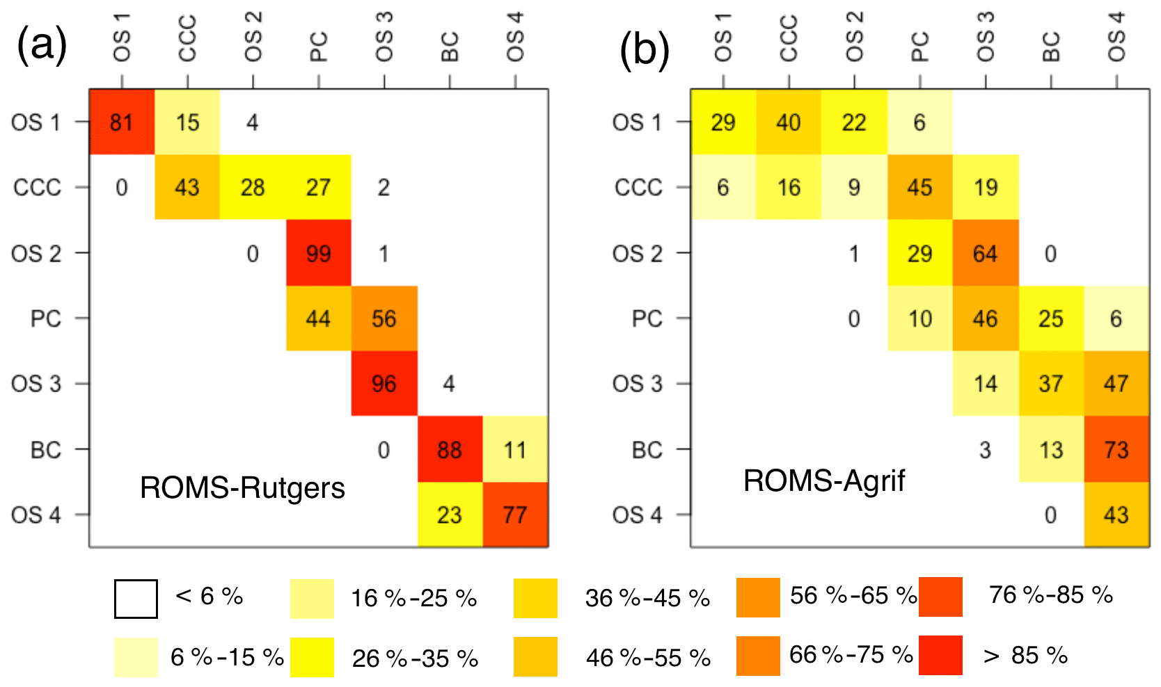
Figure 6Dispersal rate (%) of passive particles between the zones of release (y axis) and settlement (x axis). The retention rates are on the diagonal. Release zone codes are as indicated in Fig. 1.
The vertical displacement of particles at the end of the 31 d simulation was relatively independent of the bottom depth at the release event (Fig. 7). Generally, more than 26 % of particles rise above the isobath of 500 m, around 30 % of particles drifted without having vertically displaced, and 5 % of particles go deeper than 800 m (see Fig. 7). More specifically, 12.8 % of particles released above the bottom between the isobaths of 700 and 800 m (hence, 700/800 m) arrived below 800 m. There are only 0.7 % and 4.8 % of bottom-released particles between the isobaths of 500 and 600 m and the isobaths of 600 and 700 m (hence, 500/600 and 600/700 m), respectively, which also reach such a depth. Moreover, the downward displacement is greater for particles released in canyons than on open slopes. From the three depth layers, 500/600, 600/700, and 700/800 m, as previously defined, 0.2 %, 1 %, and 11.1 % of particles on open slopes and 2 %, 13.5 %, and 19.7 % of particles on canyon slopes, respectively, go deeper than 800 m. Besides, the particles released in the middle layer (600/700 m) of the canyons were likely to be more dispersed vertically than from similar release conditions on the open slope (retention on the depth 27.3 % and 36.8 %, respectively).
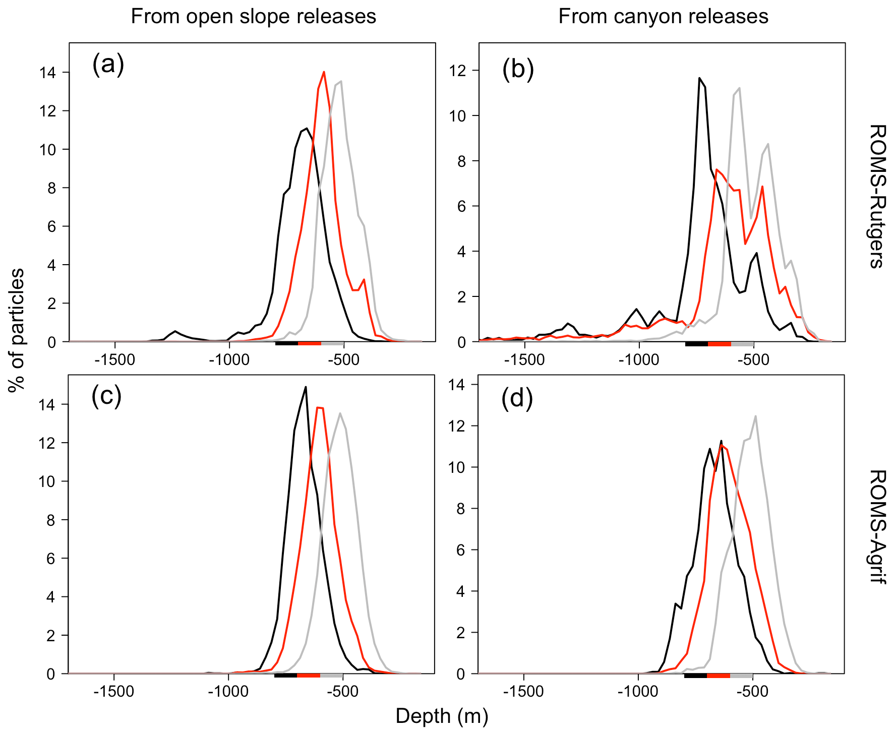
Figure 7Depth range (m) of particles after 31 d of drift. Particles were released between the following three depth ranges: 500–600 m (gray), 600–700 m (red), and 700–800 m (black) denoted by colored bars on the x axis.
In submarine canyons, the particles had a broader vertical displacement than over open slopes. Intensity and amplitudes in the vertical displacement of particles were dependent on the canyons and their walls, especially when they were released above both walls of the Blanes canyon (Fig. 8). On average, the particle vertical displacements in canyons or above the open slope are ascents of 28 and 24 m, respectively. Furthermore, the variability of the vertical displacement of particles in canyons (±154 m) is 2 times higher than on open slopes (±67.5 m). The drifts in PC have on average the highest ascent of 133 m. The PC is also the canyon with the widest vertical displacements where the maxima upward and downward displacements are 490 and 1163 m, respectively. From its southern wall, particles averagely rise 145 m, while on the northern wall there is an ascent of 58 m. Particles from the CCC averagely rose 44 m as did particles from the PC, but the vertical displacements were limited to a small range of 86 m in the CCC compared to 170 m in the PC. The drifts from BC have on average the furthest descent (127 m down). The drifts within BC went downward by 62 m when particles were above the northern wall and went upward by 36 m when particles drift above the southern wall. Contrary to the different days of release in the other canyons, the northern and southern walls of BC are where the temporal variability of the vertical displacements is the highest with a standard deviation of 53 and 34 m, respectively.
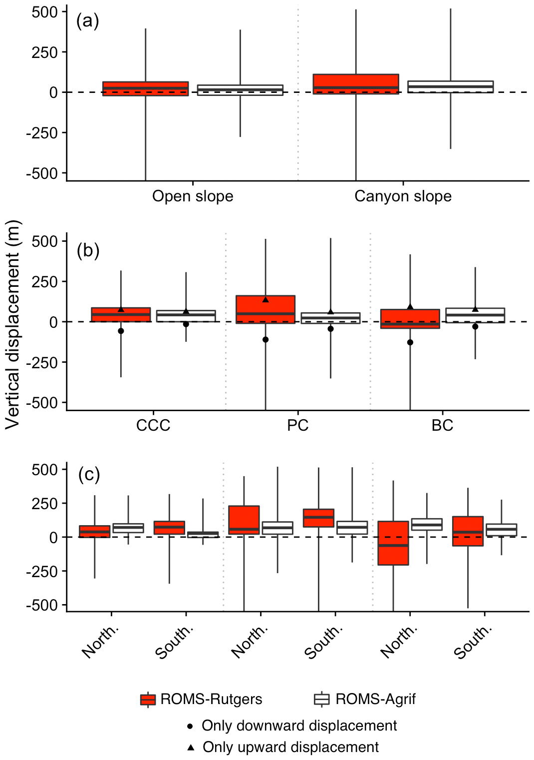
Figure 8Particles vertical displacement. Vertical displacement according to particles drifting on the open slope or the canyon slope (a), drifting within the canyons (b), and released on the northern wall (North.) or southern wall (South.) of the canyons (c) in the ROMS-Rutgers and the ROMS-Agrif simulations. Release zone codes are as indicated in Fig. 1.
The influence of submarine canyons on the transport paths resulted in a common drift direction with small divergences in the trajectories (see Fig. 9). Indeed, particles southwardly followed the continental slope and spread differently according to the canyon in which they were released. To begin with, transport paths starting in the CCC and at one depth layer (500/600, 600/700, or 700/800 m) did not overlap with the ones starting at another depth layer, and they kept a linear direction when particles left the CCC. Second, the simulated drifts that began from the PC were affected by internal circulation within the canyon (i.e., recirculation of the particles between the walls), and transport paths intersected. Last, the transport paths initialized from the BC barely left the canyon area and overlapped with the trajectories set up in a different depth layer. The overlap or intersection of the transport paths may be a consequence from the vertical displacement of the particles (see Figs. 7 and 8) that were constrained by the horizontal and vertical circulation variability (see Figs. 5 and 8).
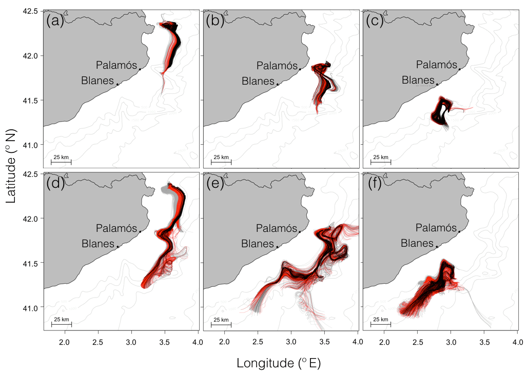
Figure 9Estimated transport paths of passive particles during 31 d. Passive particles were released in the Cap de Creus canyon (a, d), Palamós canyon (b, e), Blanes canyon (c, f), and advected by the modeled hydrodynamics from ROMS-Rutgers (a–c) and ROMS-Agrif (d–f). Colors of the transport paths are associated with the depth ranges 500–600 m (gray), 600–700 m (red), and 700–800 m (black) on which particles were released.
3.2 Lagrangian dispersal within ROMS-Agrif outputs
The particles were transported further in the ROMS-Agrif configuration than in the ROMS-Rutgers configuration (Fig. 5), and particles from the canyon zones had traveled slightly further than particles from the open slopes. The general drift distances of particles are approximately 70.8 km (±26.3 km) and 44 km longer than drift in ROMS-Rutgers. Particles could drift up to the maximum distance of 197 km, detected for particles from the PC (see Fig. 5). Among the canyons, particles from CCC were transported the least distance: 47.1 km (±21 km). Oppositely, the released particles on PC averagely travel the furthest with drifts of 84.2 km (±24.9 km). Particles from canyon slope zones or open slope zones were transported 73.7 and 68.8 km, respectively, and even though the difference of drift distances is low (5 km), it is significantly different (p<0.05). Within the canyons, the particles from the northern walls of the CCC and PC drift 66 km, which was 13 km less than the particles from the southern walls. In the BC, the tendency was for particles released on the northern wall to travel 84 km, or 10 km more than particles from the southern wall.
Southern transport of particles was on a broader scope than in ROMS-Rutgers (see Fig. 6). After a simulation period of 31 d, the retention rate by the release zones is 1 % to 43 % of particles (Fig. 6), making an average of 18 % (±14 %) of particles. Like in ROMS-Rutgers, the open slope OS 2 retains the least of particles (1 %). Consequently, a small proportion of 29 % of particles ends up in the PC, while the majority (64 %) connects with open slope OS 3. The particles from the CCC also have drifted in more zones than any other release places. They were transported in four different zones, which were OS 1 at 6 %, OS 2 at 9 %, PC at 45 %, and OS 3 at 19 %. Particularly, 45 % of particles connect to the PC and those particles are characterized by a drift of 70.5 km (±9 km) from 575 m (±77 m). A lower rate of dispersal is detected, as well, from PC to BC. On average, 25 % of particles drift approximately 86.6 km (±14.9 km) from 600 m (±82 m) to reach BC.
The pattern of vertical particle displacements in ROMS-Agrif was similar among the different release depths and topographic structures of the NW Mediterranean Sea (see Fig. 7). Overall, 37.3 % of particles reaches the layer above 500 m depth, while only 0.8 % of particles go deeper than 800 m. Particles released over the upper bottom depths (500/600 and 600/700 m) presented comparable but still significantly different (p<0.05) vertical displacements even if they were released in canyons or on open slopes. Around 41 % and 43 % of particles drifted within the same depth layer as their releases and 44 % to 48 % ascended in upper depths. On the contrary and overall, from releases between isobaths 700/800 m, a majority of the particles (65 %) went upward, a high proportion of particles (6.1 %) went down below 800 m, and fewer particles were transported in the depth layer of their release (retention in the deeper layer of 29 %).
The average vertical displacement of particles was a small ascent in the water column (see Fig. 8), with canyons being the places of higher ascents. On average, particles rose 15 m (±53 m) when released on open slopes, and twice that, 34 m (±65 m), when released in canyons. Among the different canyons, particles released in the PC were vertically displaced the least (23 m on average, or half the rise of particles from the CCC and BC), but the widest vertical displacements of 352 m downwards and 519 m upwards were from PC. We furthermore notice that the average ascent and descent of particles were the highest in BC (74 m) and in PC (44 m), respectively, which are reversed directions of movement compared to the results in ROMS-Rutgers. Lastly, particles drifting above the northern wall of all the canyons significantly (p<0.05) rise higher than for particles above the southern wall. In CCC, the rise of particles was 2.7 times higher on the northern wall (71 m) than on the southern wall, which represents the highest change in displacement between the walls. In contrast, in PC, the rise of particles reaches 68 m on the northern wall, which was 4 m less than for particles on the other wall. Over the different release dates, the southern wall of PC is where the vertical movement of particles temporally varies the most (standard deviation of 39 m).
With the simulation of passive drifts in ROMS-Agrif, patterns of particle trajectory were similar to the ones in ROMS-Rutgers, especially the southward drift direction and the spread of particles from the submarine canyons (see Fig. 9). Nonetheless, the length of the transport paths, as demonstrated by the drift distance values (see Fig. 5), was longer than in ROMS-Rutgers, and the spread of trajectories was wider. The spread was particularly amplified when particles drifted in the Palamós and Blanes canyons. For example, transport paths from the PC disclosed the advection of particles taken in two circular flows near this canyon, and the span of the transport paths from the BC widened once the particles left the canyon. Like for the simulations in ROMS-Rutgers, the variability in the transport path originated in the depth position of the particles (see Figs. 7 and 8). However, the spread of the trajectory was intensified as a consequence of the current intensity estimated in the ROMS-Agrif (see Fig. 4).
Two hydrodynamic models with different implementations allowed for testing the sensitivity of particle dispersals to the Mediterranean Sea thermohaline circulation. The dispersal rates were low and similar to observations or simulations of deep larvae from other marine ecosystems like in the Baltic Sea and in another basin of the Mediterranean Sea (Corell et al., 2012; Palmas et al., 2017).
4.1 Deep-sea connectivity between submarine canyons
For the first time in the NW Mediterranean Sea, the connectivity between submarine canyons has been demonstrated through the Lagrangian transport of deep particles. The southwestward circulation having important amplitude in upper layers also predominated in the bottom drift simulation and explained the particle trajectories from the northern canyons to the southern canyons. On a local scale (i.e., canyon area), submarine canyon areas received drifters from upstream release and seeded the nearest downstream open slopes. In fact, this result is related to the flows of the NW Mediterranean Sea following the right-hand side canyon walls (Flexas et al., 2008; Palanques et al., 2005; Granata et al., 1999; Jorda et al., 2013). With this, our drift simulations supported one of the submarine canyon functions, which consisted of seeding particles in neighboring zones.
Nonetheless, each submarine canyon has a singular topography and a different angle of exposure to the main circulation, resulting in different patterns of particle dispersals. In the horizontal dimension and inside each submarine canyon, particle drifts were different because they did not begin from the same depth, the same day, or with the same exposure to the current (i.e., releases on upstream or downstream canyon walls) even though the general canyon influence led to common north–south drift patterns. Those differences also appeared in analyses of sediment flux in the Mediterranean Sea (Durrieu de Madron et al., 1999; Lopez-Fernandez et al., 2013) and in simulations of passive particle drifts in different water layers (Ross et al., 2016). In the vertical dimension, our results reflected the uncorrelated currents occurring inside a canyon (Jorda et al., 2013) that could be one of the origins of the drift differences between canyons. For example, the amplitude of vertical drifts in Palamós canyon was greater than vertical drifts in the other canyons. The uncorrelated currents could also explain the general upward displacement of particles that were released on the upstream canyon walls. On the contrary, in shallow waters, previous flow studies on those canyon sides estimated a downward flux (Ahumada-Sempoal et al., 2015; Flexas et al., 2008; Granata et al., 1999).
Even though the main trajectory patterns persisted, canyon influence on dispersals changed over the summer releases. In Kool et al. (2015), the main deep circulation pattern over 3 years was consistent enough to not strongly impact the dispersals. This finding also applied for our results when the range of releases was over 2 months. Temporal variability around the main patterns was likely caused by the dynamic of the internal circulation over time inside the canyons (Ahumada-Sempoal et al., 2013; Palanques et al., 2005; Jorda et al., 2013). Nonetheless, further simulations of drifts need to be done to identify the minimum frequency of release to observe significant changes in the drift variability.
4.2 Sensitivity of the passive transport to deep-sea circulations
In our study, the large amplitude of dispersals in ROMS-Agrif was the main origin of differences between the drifts. Particle retention was 3.3 times higher with the simulation carried out with ROMS-Rutgers than with ROMS-Agrif. Whether the particles were released on canyon slopes or on open slopes did not change the fact that distance drifts were 2 times longer in simulations from ROMS-Agrif. The largest difference in amplitude of drifts (an average difference of 64.2 km) was simulated from the open slope between Palamós and Blanes canyons. There, in the ROMS-Rutgers bathymetric grid, the presence of a submarine valley in the slope (∼41.5∘ N, ∼3.25∘ E) lowered the dispersal rates, and acted as a wall that generated distinct dispersal lengths depending on the side on which particles were released. In contrast, on the open slope between the Cap de Creus and Palamós canyons, the continental slope did not have specific topographic structure, and in both models the zone retention was low.
Thus, small topographic differences (e.g., the submarine valley) indirectly influenced the particle transport by conditioning the flow circulation when the hydrodynamic models were run. The main cause of topographic differences was related to the resolution of the bathymetric data sets chosen by the modelers. Indeed, an adequate bathymetric data set would approximate better the mesoscale structures of the water circulation (Gula et al., 2015). Then, it made the simulated drifts from the ROMS-Rutgers more appropriate for the deep passive drifts because the bathymetric data set was more precise (i.e., horizontal resolution of 100 m instead of 3 km) even though it has a lower horizontal resolution than the ROMS-Agrif. Another major difference within the drifts in the two hydrodynamic models was the northward drifts from Blanes canyon and from the open slope at its southern end (OS4) in ROMS-Rutgers. The northward particle drift is a consequence of an anticyclonic flow generated at the mouth of Blanes canyon that also affects the local deep water circulation (Ahumada-Sempoal et al., 2013; Jorda et al., 2013). The southwestward flow in ROMS-Agrif may be the consequence of the bathymetric data set used before the run of the hydrodynamic model and the hydrodynamic model parameterization of the water profile discretization. In ROMS models, the water is discretized by terrain-following sigma layers that generally have high resolution near the surface and relax the circulation variability near the bottom.
The generated drift uncertainties gave arguments for choosing one hydrodynamic model over another, above all when drifts are in deep water. In the absence of more hydrodynamic models, we encourage the deep-sea Lagrangian modeler to cross-validate the Lagrangian drifts with the existing literature. Our work evidences the importance of two major sources of uncertainty in the particle drifts from the hydrodynamic models: bathymetry and model discretization (i.e., choice of S-coordinate parameters). These two factors are shown to be particularly important in the zones near the canyons (all the water column) and open-slope areas. This is an important outcome for modeling studies. In this sense, this study shows the areas where uncertainty grows and so helps to evaluate when and where the choice of the hydrodynamic models will have a large impact on the drift results.
4.3 Relation between deep-sea circulation and larval cycle of A. antennatus
The association of eggs and larvae of Aristeus antennatus with passive particles comprised the first approach to their drift. Our study revealed interesting dispersal features which could be related to the ecology of A. antennatus. First, few particles in canyons were transported near 1000 m depth, where peaks of juvenile abundances have been reported at the end of fall (Sardà et al., 1997; D'Onghia et al., 2009; Sardà and Cartes, 1997). It would imply that the late larvae are helped or constrained by the vertical circulation to settle in the deep zones. Second, the low dispersal rates from the canyons highlighted that inactive larvae may be retained by those topographic structures. In fact, the morphology of the canyons facilitates the retention of pelagic particles for a few days (Ahumada-Sempoal et al., 2015; Rojas et al., 2014). In that case, it would mean that subpopulations of A. antennatus strongly depend on their own. Then, the surface of management plans should be structured to local shrimp fishing grounds, like the one in Palamós canyon (Boletín Oficial del Estado, 2013, 2018). Furthermore, because the submarine valley is localized between two areas of high fishing effort (Palamós and Blanes), there is an interest in its potential role for marine populations. Literature categorizes submarine valley effects as canyon influences, but, due to the exposure of the submarine valley to the current, an evaluation of whether the valley deviates or recirculates the flow is needed.
In this study, the duration of simulation corresponded to the first PLD approximation of Aristeus antennatus larvae generalized from penaeid larvae. Nonetheless, further studies need to explore the variability of the estimated dispersal features with longer PLDs. In the framework of the A. antennatus case study, the PLD length can be expanded in accordance with a plausible time range of 6 months, i.e., time between the beginning of the spawning peak in July and the period of sampled early juveniles (Sardà et al., 1997; D'Onghia et al., 2009; Sardà and Cartes, 1997). The effect of PLD length can also be estimated with water temperature changes during the larval drift, as they are likely to affect the PLD when A. antennatus larvae reach the warm surface waters (O'Connor et al., 2007). The larval behavior needs to be taken into account, because it can significantly affect the vertical position of decapod larvae in the water column and may influence the larval dispersal (Cowen and Sponaugle, 2009; Levin, 2006; Queiroga and Blanton, 2004). Few studies on A. antennatus larvae sampled in open ocean have revealed their presence in the surface water layer (Carbonell et al., 2010; Carretón et al., 2019; Heldt, 1955; Seridji, 1971; Torres et al., 2013). Sardà et al. (2004) and Palmas et al. (2017) assumed that positive buoyancy of eggs partly underlined the presence of individuals in the shallowest water layer. The buoyancy mechanism needs to be analyzed through sensitivity tests in order to compensate for the lack of accurate knowledge about it (Hilário et al., 2015; Ross et al., 2016).
Passive drifts of particles simulated by a Lagrangian transport model coupled with two hydrodynamic models (ROMS-Rutgers and ROMS-Agrif) were compared. The particle releases used characteristics of deep-sea red shrimp, A. antennatus, spawners and scarce knowledge of their free-living period (i.e., eggs and larvae). Then, drift simulations began in a highly disturbed circulation induced by the submarine canyons of the NW Mediterranean Sea. In general, horizontal dispersion of deep-sea passive particles was relatively short during the 31 d simulation, but their transports could establish links between the submarine canyons. Like numerous other studies, our work concludes that marine topographic features (i.e., the deep submarine canyons and submarine valleys) favored particle reception and retention. It also supports that the amplitude and variability of vertical displacement (upward and downward in the water column) are higher inside submarine canyons than on other parts of the continental slope. Besides, the variability in the particle vertical displacement was dependent on the three-dimensional distribution of particle releases in a submarine canyon. Variability in particle dispersions was also a consequence of differences between canyon topography and their exposure to the currents. This sensitivity to the topography highlighted the importance of the modeler choice before running hydrodynamic models. Having a finer bathymetry data input and a finer vertical resolution near the bottom (i.e., like in ROMS-Rutgers) is important for estimating the circulation and the passive dispersions with more accuracy, even though the hydrodynamic model has a coarse horizontal resolution (i.e., 2 km vs. 1.2 km). Therefore, the ROMS-Rutgers model was approved by better modeling the bottom drifts, and it will be used for future studies on the benthic deep-sea species A. antennatus. Numerical simulations of the larval drift are one of the best approaches that allowed for approximating the unknown dispersal paths of A. antennatus in the NW Mediterranean Sea. This study is the first step of a work conducted with the final focus to improve fishery management of a deep-sea species. However, observation of the pelagic larval traits, validation of the dispersals, and simulation including biological behaviors (vertical migration, buoyancy, and swimming abilities) are required before involving the results in the management strategies.
The outputs (ROMS, script for Lagrangian model parameterization, and scripts for analysis) presented in this article are available from the first author upon request.
The supplement related to this article is available online at: https://doi.org/10.5194/os-15-1745-2019-supplement.
MCH carried out most of the research from the Lagrangian drift simulations to the analysis of the outputs. JS developed and validated the ROMS-Rutgers model. MAAS used his ROMS-Agrif model output to simulate Lagrangian drifts. FB provided codes for analyzing the Lagrangian drift sensitivity. GR and JBC guided the first author with the biology of the red shrimp. JBC is the principal researcher of CONECTA's project and provided the scholarship to MCH to realize this study. MCH prepared the article with contributions from all co-authors.
The authors declare that they have no conflict of interest.
The authors greatly thank for their time and support: Marta Carretón, the computer technicians from the Centre d’Estudis Avançats de Blanes (CEAB), and the personal from the Institut de Cienciès del Mar(ICM) at Barcelona. The authors also appreciated the numerous comments which helped to structure the article.
Funding was provided through the CONECTA project supported by the Ministerio de Economia, Industria y Competividad from the Spanish Government. Morane Clavel-Henry is funded under an FPI PhD program of the Spanish Government (grant no. BES-2015-074126).
This paper was edited by John M. Huthnance and reviewed by Xavier Durrieu de Madron and one anonymous referee.
Adani, M., Dobricic S, and Pinardi, N.: Quality assessment of a 1985–2007 Mediterranean Sea reanalysis, J. Atmos. Ocean. Tech., 28, 569–589, https://doi.org/10.1175/2010JTECHO798.1, 2011.
Ahumada-Sempoal, M. A., Flexas, M. M., Bernardello, R., Bahamon, N., and Cruzado, A.: Northern Current variability and its impact on the Blanes Canyon circulation: A numerical study, Prog. Oceanogr., 118, 61–70, https://doi.org/10.1016/j.pocean.2013.07.030, 2013.
Ahumada-Sempoal, M. A., Flexas, M. M., Bernardello, R., Bahamon, N., Cruzado, A., and Reyes Hernández, C.: Shelf-slope exchanges and particle dispersion in Blanes submarine canyon (NW Mediterranean Sea): A numerical study, Cont. Shelf Res., 109, 35–45, 2015.
Andrello, M., Mouillot, D., Beuvier, J., Albouy, C., Thuiyse, W., and Manel, S.: Low Connectivity between Mediterranean Marine Protected Areas: A Biophysical Modeling Approach for the Dusky Grouper Epinephelus marginatus, PLOS ONE, 8, e68564, https://doi.org/10.1371/journal.pone.0068564, 2013.
Arellano, S. M., Van Gaest, A. L., Johnson, S. B., Vrijenhoek, R. C., and Young, C. M.: Larvae from deep-sea methane seeps disperse in surface waters, P. Roy. Soc. B-Biol. Sci., 281, 20133276, https://doi.org/10.1098/rspb.2013.3276, 2014.
Basterretxea, G., Jordi, A., Catalán, I. A., and Sabatés, A.: Model-based assessment of local-scale fish larval connectivity in a network of marine protected areas, Fish. Oceanogr., 21, 291–306, https://doi.org/10.1111/j.1365-2419.2012.00625.x, 2012.
Boletín Oficial del Estado: Orden AAA/923/2013 de 16 de Mayo, no 126, Sec. III, 2013.
Boletín Oficial del Estado, Orden APM/532/2018 de 26 de Mayo, no 128, Sec. III, 2018.
Canals, M., Danovaro, R., Heussner, S., Lykousis, V., Puig, P., Trincardi, F., and Sanchez-Vidal, A.: Cascades in Mediterranean submarine grand canyons, Oceanography, 22, 26–43, 2009.
Carbonell, A., Dos Santos, A., Alemany, F., and Vélez-Belchi, P.: Larvae of the red shrimp Aristeus antennatus (Decapoda: Dendrobranchiata: Aristeidae) in the Balearic Sea: new occurrences fifty years later, Mar. Biodivers. Rec., 3, E103, https://doi.org/10.1017/s1755267210000758, 2010.
Carretón, M., Company, J. B., Planella, L., Heras, S., García-Marín, J. L., Agulló, M., Clavel-Henry, M., Rotllant, G., dos Santos, A., and Roldán, M. I.: Morphological identification and molecular confirmation of the deep-sea blue and red shrimp Aristeus antennatus larvae, Peer J., 7, e6063, https://doi.org/10.7717/peerj.6063, 2019.
Chen, C., Liu, H., and Beardsley, R. C.: An Unstructured Grid, Finite-Volume, Three-Dimensional, Primitive Equations Ocean Model: Application to Coastal Ocean and Estuaries, J. Atmos. Ocean. Tech., 20, 159–186, https://doi.org/10.1175/1520-0426(2003)020<0159:AUGFVT>2.0.CO;2, 2003.
Coll, M., Steenbeek, J., Solé, J., Palomera, I., and Christensen, W.: Modelling the cumulative spatial–temporal effects of environmental drivers and fishing in a NW Mediterranean marine ecosystem, Ecol. Modell., 331, 100–114, https://doi.org/10.1016/j.ecolmodel.2016.03.020, 2016.
Corell, H., Moksnes, P. O., Engqvist, A., Döös, K., and Jonsson, P. R.: Depth distribution of larvae critically affects their dispersal and the efficiency of marine protected areas, Mar. Ecol. Prog. Ser., 467, 29–46, 2012.
Cowen, R. K. and Sponaugle, S.: Larval dispersal and marine population connectivity, Annu. Rev. Mar. Sci., 1, 443–466, https://doi.org/10.1146/annurev.marine.010908.163757, 2009.
Cromey, C. J. and Black, K. D.: Modelling the Impacts of Finfish Aquaculture, in: Environmental Effects of Marine Finfish Aquaculture, edited by: Hargrave B. T., Handbook of Environmental Chemistry, vol 5M, Springer, Berlin, Heidelberg, 129–155, 2005.
Dall, W.: The biology of the Penaeidae, Adv. Mar. Biol., 27, 489 pp., 1990.
Debreu, L., Marchesiello, P., Penven, P., and Cambon, G.: Two-way nesting in split-explicit ocean models: algorithms, implementation and validation, Ocean Modell., 49–50, 1–21, https://doi.org/10.1016/j.ocemod.2012.03.003, 2012.
Dee, D. P., Uppala, S. M., Simmons, A. J., Berrisford, P., Poli, P., Kobayashi, S., Andrae, U., Balmaseda, M. A., Balsamo, G., Bauer, P., Bechtold, P., Beljaars, A. C. M., van de Berg, L. Bidlot, J., Bormann, N., Delsol, C., Dragani, R., Fuentes, M., Geer, A. J., Haimberger, L., Healy, S. B., Hersbach, H., Hólm, E. V., Isaksen, L., Kållberg, P., Köhler, M., Matricardi, M., McNally, A. P., Monge-Sanz, B. M., Morcrette, J.-J., Park, B.-K.,Peubey, C.,de Rosnay, P., Tavolato, C., Thépaut, J.-N., and Vitart, F.: The ERA-Interim reanalysis: configuration and performance of the data assimilation system, Q. J. Roy. Meteorol. Soc., 137, 553–597, https://doi.org/10.1002/qj.828, 2011.
Demestre, M. and Fortuno, J. M.: Reproduction of the deep-water shrimp Aristeus antennatus (Decapoda: Dendrobranchiata), Mar. Ecol. Prog. Ser., 84, 41–51, 1992.
Demestre, M. and Lleonart, J.: Population dynamics of Aristeus antennatus (Decapoda: Dendrobranchiata) in the northwestern Mediterranean, Sci. Mar., 57, 183–189, 1993.
D'Onghia, G., Maiorano, P., Capezzuto, F., Carlucci, R., Battista, D., Giove, A., and Tursi, A.: Further evidences of deep-sea recruitment of Aristeus antennatus (Crustacea: Decapoda) and its role in the population renewal on the exploited bottoms of the Mediterranean, Fish. Res., 95, 236–245, https://doi.org/10.1016/j.fishres.2008.09.025, 2009.
Durrieu de Madron, X., Radakovitch, O., Heussner, S., Loye-Pilot, M. D., and Monaco, A.: Role of the climatological and current variability on shelf-slope exchanges of particulate matter: Evidence from the Rhône continental margin (NW Mediterranean), Deep-Sea Res. Pt. I, 46, 1513–1538, https://doi.org/10.1016/S0967-0637(99)00015-1, 1999.
Etter, R. J. and Bower, A. S.: Dispersal and population connectivity in the deep North Atlantic estimated from physical transport processes, Deep-Sea Res. Pt. I, 104, 159–172, https://doi.org/10.1016/j.dsr.2015.06.009, 2015.
Fairall, C. W., Bradley, E. F., Rogers, D. P., Edson, J. B., and Young, G. S.: Bulk parameterization of air-sea fluxes for tropical ocean-global atmosphere coupled-ocean atmosphere response experiment, J. Geophys. Res., 101, 3747–3764, https://doi.org/10.1029/95JC03205, 1996.
Fernandez-Arcaya, U., Ramirez-Llodra, E., Aguzzi, J., Allcock, A. L., Davies, J. S., Dissanayake, A., and Van den Beld, I. M. J.: Ecological Role of Submarine Canyons and Need for Canyon Conservation: A Review, Front. Mar. Sci., 4, 26, https://doi.org/10.3389/fmars.2017.00005, 2017.
Flexas, M. M., Boyer, D. L., Espino, M., Puigdefábregas, J., Rubio, A., and Company, J. B.: Circulation over a submarine canyon in the NW Mediterranean, J. Geophys. Res., 113, C12002, https://doi.org/10.1029/2006JC003998, 2008.
Gorelli, G., Company, J. B., and Sardà, F.: Management strategies for the fishery of the red shrimp Aristeus antennatus in Catalonia (NE Spain), Marine Stewardship Council Science Series, 2, 116–127, 2014.
Granata, T. C., Vidondo, B., Duarte, C. M., Satta, M. P., and Garcia, M.: Hydrodynamics and particle transport associated with a submarine canyon off Blanes (Spain), NW Mediterranean Sea, Cont. Shelf Res., 19, 1249–1263, https://doi.org/10.1016/S0278-4343(98)00118-6, 1999.
Gula, J., Molemaker, M. J., and McWilliams, J. C.: Topographic vorticity generation, submesoscale instability and vortex street formation in the Gulf Stream, Geophys. Res. Lett., 42, 4054–4062, 2015.
Heldt, J. H.: Contribution à l'étude de la biologie des crevettes pénéides: Aristaeomorpha foliacea (Risso) et Aristeus antennatus (Risso), formes larvaires, Bulletin de la Société des Sciences Naturelles de Tunisie, VIII(1–2), 1–29, 1955.
Hilário, A., Metaxas, A., Gaudron, S., Howell, K., Mercier, A., Mestre, N., and Young, C.: Estimating dispersal distance in the deep sea: challenges and applications to marine reserves, Front. Mar. Sci., 2, 14, https://doi.org/10.3389/fmars.2015.00006, 2015.
Jones, C. E., Dagestad, K.-F., Breivik, Ø., Holt, B., Röhrs, J., Christensen, K. H., and Skrunes, S.: Measurement and modeling of oil slick transport, J. Geophys. Res.-Oceans, 121, 7759–7775, https://doi.org/10.1002/2016JC012113, 2016.
Jorda, G., Flexas, M. M., Espino, M., and Calafat, A.: Deep flow variability in a deeply incised Mediterranean submarine valley (Blanes canyon), Prog. Oceanogr., 118, 47–60, https://doi.org/10.1016/j.pocean.2013.07.024, 2013.
Jordi, A., Basterretxea, G., Orfila, A., and Tintoré, J.: Analysis of the circulation and shelf-slope exchanges in the continental margin of the northwestern Mediterranean, Ocean Sci., 2, 173–181, https://doi.org/10.5194/os-2-173-2006, 2006.
Kool, J. T., Huang, Z., and Nichol, S. L.: Simulated larval connectivity among Australian southwest submarine canyons, Mar. Ecol. Prog. Ser., 539, 77–91, 2015.
Kough, A. S., Paris, C. B., and Butler IV, M. J.: Larval connectivity and the International Management of fisheries, PLOS ONE, 8, e64970, https://doi.org/10.1371/journal.pone.0064970, 2013.
Large, W., McWilliams, J., and Doney, S.: Oceanic vertical mixing: a review and a model with a nonlocal boundary layer parameterization, Rev. Geophys., 32, 363–403, 1994.
Lebreton, L. C. M., Greer, S. D., and Borrero, J. C.: Numerical modelling of floating debris in the world's oceans, Mar. Pollut. Bull., 64, 653–661, 2012.
Lett, C., Verley, P., Mullon, C., Parada, C., Brochier, T., Penven, P., and Blanke, B. A.: Lagrangian tool for modelling ichthyoplankton dynamics, Environ. Modell. Soft., 23, 1210–1214, https://doi.org/10.1016/j.envsoft.2008.02.005, 2008.
Levin, L. A. and Bridges, T. S.: Pattern and diversity in reproduction and development, edited by: McEdward, L., CRC Press, Boca Raton, 1995.
Levin, L. A.: Recent progress in understanding larval dispersal: new directions and digressions, Integr. Comparat. Biol., 46, 282–297, https://doi.org/10.1093/icb/icj024, 2006.
Lopez-Fernandez, P., Calafat, A., Sanchez-Vidal, A., Canals, M., Mar Flexas, M., Cateura, J., and Company, J. B.: Multiple drivers of particle fluxes in the Blanes submarine canyon and southern open slope: Results of a year round experiment, Prog. Oceanogr., 118, 95–107, https://doi.org/10.1016/j.pocean.2013.07.029, 2013.
Millot, C.: Circulation in the Western Mediterranean Sea, J. Mar. Syst., 20, 423–442, 1999.
North, E. W.: Vertical swimming behavior influences the dispersal of simulated oyster larvae in a coupled particle-tracking and hydrodynamic model of Chesapeake Bay, Mar. Ecol. Prog. Ser., 359, 99–115, https://doi.org/10.3354/meps07317, 2008.
North, E. W., Gallego, A., and Petitgas, P.: Manual of recommended practices for modelling physical-biological interactions during fish early life, ICES Cooperative Research Report, 295, 111 pp., 2009.
O'Connor, M. I., Bruno, J. F., Gaines, S. D., Halpern, B. S., Lester, S. E., Kinlan, B. P., and Weiss, J. M.: Temperature control of larval dispersal and the implications for marine ecology, evolution, and conservation, P. Natl. Acad. Sci. USA, 104, 1266–1271, https://doi.org/10.1073/pnas.0603422104, 2007.
Ospina-Álvarez, A., Bernal, M., Catalán, I. A., Roos, D., Bigot, J.-L., and Palomera, I.: Modeling Fish Egg Production and Spatial Distribution from Acoustic Data: A Step Forward into the Analysis of Recruitment, PLOS ONE, 8, e73687, https://doi.org/10.1371/journal.pone.0073687, 2013.
Palanques, A., García-Ladona, E., Gomis, D., Martín, J., Marcos, M., Pascual, A., and Pagès, F.: General patterns of circulation, sediment fluxes and ecology of the Palamós (La Fonera) submarine canyon, northwestern Mediterranean, Prog. Oceanogr., 66, 89–119, https://doi.org/10.1016/j.pocean.2004.07.016, 2005.
Palmas, F., Olita, A., Addis, P., Sorgente, R., and Sabatini, A.: Modelling giant red shrimp larval dispersal in the Sardinian seas: density and connectivity scenarios, Fish. Oceanogr., 26, 364–378, https://doi.org/10.1111/fog.12199, 2017.
Paris, C. B., Helgers, J., van Sebille, E., and Srinivasan, A.: Connectivity Modeling System: A probabilistic modeling tool for the multi-scale tracking of biotic and abiotic variability in the ocean, Environ. Modell. Soft., 42, 47–54, https://doi.org/10.1016/j.envsoft.2012.12.006, 2013.
Penven, P., Marchesiello, P., Debreu, L., and Lefèvre, J.: Software tools for pre- and post-processing of oceanic regional simulations, Environ. Modell. Soft., 23, 660–662, https://doi.org/10.1016/j.envsoft.2007.07.004, 2008.
Pepin, P.: Effect of Temperature and Size on Development, Mortality, and Survival Rates of the Pelagic Early Life History Stages of Marine Fish, Can. J. Fish. Aquat. Sci., 48, 503–518, https://doi.org/10.1139/f91-065, 1991.
Puig, P., Ogsto, A. S., Mullenbach, B. L., Nittrouer, C. A., and Sternberg, R. W.: Shelf-to-canyon sediment transport processes on the Eel Continental Margin (Nothern California), Mar. Geol., 193, 129–149, 2003.
Qiu, Z. F., Doglioli, A. M., He, Y. J., and Carlotti, F.: Lagrangian model of zooplankton dispersion: numerical schemes comparisons and parameter sensitivity tests, Chin. J. Oceanol. Limn., 29, 438–445, https://doi.org/10.1007/s00343-011-0015-9, 2011.
Queiroga, H. and Blanton, J.: Interactions Between Behaviour and Physical Forcing in the Control of Horizontal Transport of Decapod Crustacean Larvae, Adv. Mar. Biol., 47, 107–214, 2004.
Rojas, P., Garcia, M.A., Sospedra, J., Figa, J., De Fàbregas, J., López, O., Espino, M., Ortiz, V., Sanchez-Arcilla, A., Manriquez, M., and Shirasago, B.: On the structure of the mean flow in the Blanes Canyon Area (NW Mediterranean) during summer, Oceanologica Acta, 18, 443–454, 1995.
Rojas, P. M. and Landaeta, M. F.: Fish larvae retention linked to abrupt bathymetry at Mejillones Bay (northern Chile) during coastal upwelling events, Lat. Am. J. Aquat. Res., 42, 989–1008, 2014.
Ross, R. E., Nimmo-Smith, W. A. M, and Howell, K. L.: Increasing the Depth of Current Understanding: Sensitivity Testing of Deep-Sea Larval Dispersal Models for Ecologists, PLOS ONE, 11, e0161220, https://doi.org/10.1371/journal.pone.0161220, 2016.
Sardà, F. and Cartes, J. E.: Morphological features and ecological aspects of early juvenile specimens of the aristeid shrimp Aristeus antennatus (Risso, 1816), Mar. Freshwater Res., 48, 73–77, https://doi.org/10.1071/MF95043, 1997.
Sardà, F. and Company, J. B.: The deep-sea recruitment of Aristeus antennatus (Risso, 1816) (Crustacea: Decapoda) in the Mediterranean Sea, J. Mar. Syst., 105–108, 145–151, https://doi.org/10.1016/j.jmarsys.2012.07.006, 2012.
Sardà, F., Maynou, F., and Tallo, L.: Seasonal and spatial mobility patterns of rose shrimp Aristeus antennatus in the western Mediterranean: results of a long-term study, Mar. Ecol.-Prog. Ser., 159, 133–141, 1997.
Sardà, F., D'Onghia, G., Politou, C. Y., Company, J. B., Maiorano, P., and Kapiris, K.: Deep-sea distribution, biological and ecological aspects of Aristeus antennatus (Risso, 1816) in the Western and Central Mediterranean Sea, Sci. Mar., 68, 117–127, 2004.
Schram, F., von Vaupel Klein, C., Charmantier-Daures, M., and Forest, J.: Treatise on Zoology – Anatomy, Taxonomy, Biology, The Crustacea, Volume 9 Part A: Eucarida: Euphausiacea, Amphionidacea, and Decapoda (partim), Brill, Leiden, the Netherlands, 2010.
Seridji, R.: Contribution à l'étude des larves crustacés décapods en Baie d'Alger, Pelagos, 3, 1–105, 1971.
Shan S., Sheng J., and Greenan B. J. W.: Physical processes affecting circulation and hydrography in the Sable Gully of Nova Scotia, Deep-Sea Res. Pt. II, 104, 35–50, 2014.
Shchepetkin, A. A.: Method for computing horizontal pressure-gradient force in an oceanic model with a nonaligned vertical coordinate, J. Geophys. Res., 108, 3090, https://doi.org/10.1029/2001JC001047, 2003.
Shchepetkin, A. F. and McWilliams, J. C.: The regional oceanic modeling system (ROMS): a split-explicit, free-surface, topography-following-coordinate oceanic model, Ocean Modell., 9, 347–404, https://doi.org/10.1016/j.ocemod.2004.08.002, 2005.
Siegel, D. A., Kinlan, B. P., Gaylord, B., and Gaines, S. D.: Lagrangian descriptions of marine larval dispersion, Mar. Ecol. Prog. Ser., 260, 83–96, 2003.
Simons, R. D., Siegel, D. A., and Brown, K. S.: Model sensitivity and robustness in the estimation of larval transport: A study of particle tracking parameters, J. Mar. Syst., 119–120, 19–29, https://doi.org/10.1016/j.jmarsys.2013.03.004, 2013.
Smith, W. H. F. and Sandell, D. T.: Global seafloor topography from satellite altimetry and ship depth soundings, Science, 277, 1957–1962, 1997.
Smolarkiewicz, P. K. and Margolin L. G.: MPDATA: A finite-difference solver for geophysical flows, J. Comput. Phys., 140, 459–480, https://doi.org/10.1006/jcph.1998.5901, 1998.
Solé, J., Ballabrera-Poy, J., Macías, D., and Catalán, I. A.: The role of ocean velocities in chlorophyll variability. A modeling study in the Alboran Sea, Sci. Mar., 80, 249–256, https://doi.org/10.3989/scimar.04290.04A, 2016.
Solé, J., Emelianov, M., García-Ladona, E., Ostrovskii, A., and Puig, P.: Fine-scale water mass variability inside a narrow submarine canyon (the Besòs Canyon) in the NW Mediterranean Sea, Sci. Mar., 80, 195–204, https://doi.org/10.3989/scimar.04322.05A, 2016.
Taylor, K. E.: Summarizing multiple aspects of model performance in a single diagram, J. Geophys. Res.-Atmos., 106, 7183–7192, 2001.
Thatje, S., Bacardit, R., and Arntz, W.: Larvae of the deep-sea Nematocarcinidae (Crustacea: Decapoda: Caridea) from the Southern Ocean, Polar Biol., 28, 290–302, https://doi.org/10.1007/s00300-004-0687-0, 2005.
Torres, A. P., Santos, A., Alemany, F., and Massutí, E.: Larval stages of crustacean species of interest for conservation and fishing exploitation in the Western Mediterranean, Sci. Mar., 77, 149–160, https://doi.org/10.3989/scimar.03749.26D, 2013.
Tudela, S., Sardà, F., Maynou, F., and Demestre, M.: Influence of Submarine Canyons on the Distribution of the Deep-Water Shrimp, Aristeus antennatus (Risso, 1816) in the NW Mediterranean, Crustaceana, 76, 217–225, 2003.
Uppala, S. M., KÅllberg, P. W., Simmons, A. J., Andrae, U., Bechtold, V. D. C., Fiorino, M., Gibson, J. K., Haseler, J., Hernandez, A., Kelly, G. A., Li, X., Onogi, K., Saarinen, S., Sokka, N., Allan, R. P., Andersson, E., Arpe, K., Balmaseda, M. A., Beljaars, A. C. M., Berg, L. V. D., Bidlot, J., Bormann, N., Caires, S., Chevallier, F., Dethof, A., Dragosavac, M., Fisher, M., Fuentes, M., Hagemann, S., Hólm, E., Hoskins, B. J., Isaksen, L., Janssen, P. A. E. M., Jenne, R., Mcnally, A. P., Mahfouf, J.-F., Morcrette, J.-J., Rayner, N. A., Saunders, R. W., Simon, P., Sterl, A., Trenberth, K. E., Untch, A., Vasiljevic, D., Viterbo, P., and Woollen, J.: The ERA-40 re-analysis, Q. J. Roy. Meteorol. Soc., 131, 2961–3012, https://doi.org/10.1256/qj.04.176, 2005.
Williamson, D. I.: Larval morphology and diversity, in: The Biology of Crustacea, edited by: Abele, L. G., Vol. 2, Embryology, Morphology, and Genetics, Academic Press, New York, 489 pp., 1982.
Young, C. M., He, R., Emlet, R. B., Li, Y., Qian, H., Arellano, S. M., and Rice, M. E.: Dispersal of Deep-Sea Larvae from the Intra-American Seas: Simulations of Trajectories using Ocean Models, Integr. Comparat. Biol., 52, 483–496, https://doi.org/10.1093/icb/ics090, 2012.