Isoneutral control of effective diapycnal mixing in numerical ocean models with neutral rotated diffusion tensors

Hochet, Antoine; Tailleux, Rémi; Ferreira, David; Kuhlbrodt, Till

doi:https://doi.org/10.5194/os-15-21-2019

Articles | Volume 15, issue 1

https://doi.org/10.5194/os-15-21-2019

Articles | Volume 15, issue 1

Research article

09 Jan 2019

Research article |

| 09 Jan 2019

Isoneutral control of effective diapycnal mixing in numerical ocean models with neutral rotated diffusion tensors

Antoine Hochet, Rémi Tailleux, David Ferreira, and Till Kuhlbrodt

Abstract

It is well known that there is an infinite number of ways of constructing a globally defined density variable for the ocean, with each possible density variable having, a priori, its own distinct diapycnal diffusivity. Because no globally defined density variable can be exactly neutral, numerical ocean models tend to use rotated diffusion tensors mixing separately in the directions parallel and perpendicular to the local neutral vector at rates defined by the isoneutral and dianeutral mixing coefficients respectively. To constrain these mixing coefficients from observations, one widely used tool is inverse methods based on Walin-type water mass analyses. Such methods, however, can only constrain the diapycnal diffusivity of the globally defined density variable γ – such as σ₂ – that underlies the inverse method. To use such a method to constrain the dianeutral mixing coefficient therefore requires understanding the relations between the different diapycnal diffusivities. However, this is complicated by the fact that the effective diapycnal diffusivity experienced by γ is necessarily partly controlled by isoneutral diffusion owing to the unavoidable misalignment between iso-γ surfaces and the neutral directions. Here, this effect is quantified by evaluating the effective diapycnal diffusion coefficient pertaining to five widely used density variables: γⁿ of Jackett and McDougall (1997); the Lorenz reference state density ρ_ref of Saenz et al. (2015); and three potential density variables σ₀, σ₂ and σ₄. Computations are based on the World Ocean Circulation Experiment climatology, assuming either a uniform value for the isoneutral mixing coefficient or spatially varying values inferred from an inverse calculation. Isopycnal mixing contributions to the effective diapycnal mixing yield values consistently larger than 10⁻³ m² s⁻¹ in the deep ocean for all density variables, with γⁿ suffering the least from the isoneutral control of effective diapycnal mixing and σ₀ suffering the most. These high values are due to spatially localised large values of non-neutrality, mostly in the deep Southern Ocean. Removing only 5 % of these high values on each density surface reduces the effective diapycnal diffusivities to less than 10⁻⁴ m² s⁻¹. The main implication of this work is to highlight the conceptual and practical difficulties of relating the diapycnal mixing diffusivities inferred from global budgets or inverse methods relying on Walin-like water mass analyses to locally defined dianeutral diffusivities. Doing so requires the ability to separate the relative contribution of isoneutral mixing from the effective diapycnal mixing. Because it corresponds to a special case of Walin-type water mass analysis, the determination of spurious diapycnal mixing based on monitoring the evolution of the Lorenz reference state may also be affected by the above issues when using a realistic nonlinear equation of state. The present results thus suggest that part of previously published spurious diapycnal mixing estimates could be due to isoneutral mixing contamination.

Download & links

Article (PDF, 1619 KB)

Download & links

How to cite.

Received: 13 Jul 2017 – Discussion started: 28 Aug 2017 – Revised: 26 Nov 2018 – Accepted: 29 Nov 2018 – Published: 09 Jan 2019

1 Introduction

Tracers in the oceans are stirred and mixed preferentially along isopycnal surfaces Iselin (1939); Montgomery (1940); Solomon (1971). This process is associated with a forward cascade of tracer variance to smaller scales, ultimately leading to molecular diffusion. In coarse-resolution ocean models this is a sub-grid-scale process that must be parameterised. In such models, it is common practice (Redi, 1982) to mix potential temperature (alternatively conservative temperature) and salinity¹ by means of a rotated diffusion tensor aligned with the local neutral direction. Note that sub-grid-scale mixing processes in ocean models include two other important components: dianeutral mixing and eddy-induced advection. It is now well-established that sub-grid-scale mixing processes are of key importance for climate change simulations, as they directly control ocean heat uptake, the strength of the Atlantic meridional overturning circulation and the poleward heat transport Gnanadesikan et al. (2015); Kuhlbrodt and Gregory (2012); Pradal and Gnanadesikan (2014).

A conceptual difficulty with neutral rotated diffusion tensors, however, is that it is not possible to construct a well-defined and materially conserved density variable γ(S,θ) whose gradient is parallel to the neutral direction everywhere (McDougall and Jackett, 1988 b). Mathematically, the problem arises because the local concept of neutral mixing cannot be extended globally (see Appendix A).

This implies that the “effective cross-isopycnal mixing” experienced by a material density variable γ(S,θ), that is, the local diffusive flux of γ through an iso-γ surface (i.e. γ=constant) must at least be partly controlled by isoneutral mixing. This control depends on the degree of non-neutrality of the density variable considered (Fig. 1).

In other words, the diapycnal mixing seen by any isopycnal surface, including the neutral surfaces γⁿ of Jackett and McDougall (1997), is “contaminated” by the isoneutral mixing.

Although the issue was raised before (Lee et al., 2002; McDougall and Jackett, 2005), the idea that the effective diapycnal diffusivity experienced by any mathematically globally defined density variable might be contaminated by isoneutral mixing is not widely recognized in studies estimating diapycnal mixing, whether it is spurious numerical mixing in models (Griffies et al., 2000; Ilıcak et al., 2012; Lee et al., 2002; Megann, 2018) or an inversion and Walin-like estimate of effective mixing in models or observations (Nurser et al., 1999).

A quantification of this effect in terms of diapycnal diffusion is the first aim of this work. To do so, we develop a mathematical framework to estimate the implied diapycnal mixing due to isoneutral mixing on any density surface. Using the observed ocean climatology, we then quantify the contamination of diapycnal diffusion by isoneutral mixing for a series of commonly used density surfaces. We will consider the following: γⁿ of Jackett and McDougall (1997); three potential density variables σ₀, σ₂ and σ₄; and the Lorenz reference state density ρ_ref. Note that although the ω surfaces of Klocker et al. (2009) are more neutral than γⁿ, no density variable associated with ω surfaces has been constructed yet. This makes the use of the latter impractical for the present purposes. These density variables have been chosen because they are widely used in the oceanographic community and thus deserve special attention.

Our results provide the first estimate of the uncertainties associated with diagnosing diapycnal mixing in the presence of isoneutral mixing. They further suggest that their effect might, in fact, be more important than usually assumed, therefore warranting more attention than it has received. Another motivation stems from a recent justification for the well-known one-dimensional advection–diffusion model for heat uptake in the ocean, e.g. Huber et al. (2015), in which the diapycnal diffusivity diffusing heat downward is the effective diapycnal diffusivity discussed in a current paper (see https://arxiv.org/abs/1708.02085 – last access: 2 January 2019).

The present work also raises questions about how to measure and interpret the measurement of diapycnal mixing. Indeed measured diapycnal mixing is not easily separated from isoneutral mixing and depends on the choice of density surface used for the diagnostic. Related to that, the mathematical framework we use below clearly reveals that for a given turbulent flux, an infinite number of projections and thus of iso-diapycnal diffusion coefficients, each associated to a choice of density surface, are possible.

Section 2 presents the theoretical framework used for defining effective diffusivities for each variable. We also discuss how our framework relates to similar concepts and approaches previously published. Section 3 presents estimates of the diapycnal diffusion contamination due to isoneutral mixing for the aforementioned five density variables. The sensitivity of the results to the choice of isoneutral mixing and location is also discussed. In Sect. 4, we discuss the wider implications of our findings and the related issue of defining, measuring and comparing mixing coefficients. Section 5 summarizes and discusses the results.

2 Method

2.1 Effective diffusivity

Thermodynamic properties in numerical ocean models are commonly formulated in terms of θ and S, whose evolution equations can in general be expressed as:

\begin{matrix} (1) & \frac{D_{res} θ}{D t} = \nabla \cdot (K \nabla θ) + f_{θ}, \frac{D_{res} S}{D t} = \nabla \cdot (K \nabla S) + f_{S}, \end{matrix}

where $K = K_{i} (I - d \cdot d^{T}) + K_{d} d \cdot d^{T}$ is the neutral rotated diffusion tensor of Redi (1982) (with K_i and K_d being the isoneutral and dianeutral turbulent mixing coefficients respectively, $d = N / | N |$ is the locally defined normalised neutral vector), f_S and f_θ are respectively the forcing terms for salinity and potential temperature, and $D_{res} / D t = \partial / \partial t + (v + v^{⋆}) \cdot \nabla$ is the advection by the residual velocity (the sum of the Eulerian velocity and the mesoscale eddy-induced velocity). A common parameterisation for v^⋆ is that of Gent and McWilliams (1990; see also Griffies, 2004), however the following arguments are independent of the precise form of v^⋆. Note here that K_i and K_d are implicitly defined in terms of the orthogonal projections of the turbulent heat and salt fluxes on the isoneutral and dianeutral directions; for an alternative and more recent definition of K_i and K_d aimed at making dianeutral mixing appear to be isotropic, see McDougall et al. (2014). For clarity, the directions parallel and perpendicular to the local neutral tangent planes are referred to as “dianeutral” and “isoneutral” respectively, with the terms “diapycnal” and “isopycnal” being used when isopycnal surfaces are defined in terms of a material density variable $γ (S, θ) = constant$ .

The evolution equation of any material density variable γ(S,θ) is

\begin{array}{l} \frac{D_{res} γ}{D t} = \nabla \cdot (K \nabla γ) \\ (2) & - \underset{NL}{\underset{︸}{(γ_{θ θ} \nabla θ^{T} K \nabla θ + 2 γ_{S θ} \nabla S^{T} K \nabla θ + γ_{S S} \nabla S^{T} K \nabla S)}} . \end{array}

Unless γ(S,θ) is a linear function of S and θ, its evolution equation will generally contain non-vanishing nonlinear terms (denoted as NL in Eq. 2) related to cabbeling and thermobaricity, e.g. McDougall (1987), Klocker and McDougall (2010) and Urakawa et al. (2013).

The diffusive flux of γ is

\begin{matrix} (3) & F_{diff}^{γ} = - K \nabla γ = \underset{F_{diff}^{i}}{\underset{︸}{- K_{i} (\nabla γ - (\nabla γ \cdot d) d)}} \underset{F_{diff}^{d}}{\underset{︸}{- K_{d} (\nabla γ \cdot d) d}}, \end{matrix}

where $F_{diff}^{i}$ and $F_{diff}^{d}$ are respectively the diffusive flux of γ in the isoneutral and dianeutral direction. For clarity, Fig. 1 shows a schematic of the neutral plane, of the $γ = const .$ plane, of the ∇γ and neutral direction, and of $F_{diff}^{i}$ and $F_{diff}^{d}$ .

https://www.ocean-sci.net/15/21/2019/os-15-21-2019-f01

Figure 1Schematic showing the neutral plane and neutral direction d in blue, the $γ = const .$ plane and ∇γ direction in black, and the projection of the diffusive flux of γ in the isoneutral $(F_{diff}^{i})$ and dianeutral $(F_{diff}^{d})$ direction.

Download

We define the effective diffusive flux of γ as the integral of the diffusive flux across the isopycnal surface $γ (x, t) = constant$ , viz.,

\begin{matrix} (4) & F_{eff} = - \int_{γ = const} K \nabla γ \cdot n d S, \end{matrix}

where $n = \frac{\nabla γ}{| \nabla γ |}$ is the local unit normal vector to the γ surface. Now, it is easily established after some straightforward algebra that

\begin{matrix} (5) & \begin{array}{ll} K \nabla γ \cdot n & = [K_{i} (\nabla γ - (\nabla γ \cdot d) d) + K_{d} (\nabla γ \cdot d) d] \cdot \frac{\nabla γ}{| \nabla γ |} \\ = [K_{i} (| \nabla γ |^{2} - (\nabla γ \cdot d)^{2}) + K_{d} (\nabla γ \cdot d)^{2}] / | \nabla γ | \\ = | \nabla γ | [K_{i} \sin^{2} (\nabla γ, d) + K_{d} \cos^{2} (\nabla γ, d)] . \end{array} \end{matrix}

Equation (5) establishes that the locally defined effective diapycnal diffusivity experienced by the density variable γ is affected by both isoneutral and dianeutral mixing, the contribution from isoneutral mixing being akin to a Veronis-like effect, as discussed in Tailleux (2016). Because we are primarily interested in the latter effect, we discard the effect of dianeutral mixing on the effective diapycnal diffusivity of γ and hence assume K_d=0 in the rest of the paper. As a result, the expression for the effective diapycnal diffusive flux of γ due to isoneutral mixing becomes

\begin{matrix} (6) & F_{eff} = - \int_{γ = const} | \nabla γ | K_{i} \sin^{2} (\nabla γ, d) d S . \end{matrix}

The integrand of Eq. (6) is mathematically equivalent to what McDougall and Jackett (2005) refer to as “fictitious diapycnal mixing”. However, here the integrand is integrated on γ surfaces and is then used to calculate an effective diffusivity coefficient, which is easier to interpret than a collection of local values of the (∇γ,d) angle.

2.2 Reference profile

To construct an effective turbulent diffusivity K_eff associated with the effective diffusivity flux F_eff, we need to define an appropriate mean gradient for the density variable γ. This is done by constructing a reference profile for γ, as explained in the next paragraph.

Let z_r(γ,t) be the reference profile for the particular material density γ(S,θ) (which can always be written as a function of space x and time t as $γ^{*} (x, t) = γ (S (x, t), θ (x, t))$ , constructed to be the implicit solution to the following problem:

\begin{matrix} (7) & \int_{V (z_{r})} d V = \int_{V (γ, t)} d V = \int_{z_{r} (γ, t)}^{0} A (z) d z, \end{matrix}

where A(z) is the depth-dependent area of the ocean at depth z, and V(γ,t) is the volume of water for all parcels with density γ₀ such that γ₀≤γ. The knowledge of the reference profile allows one to regard the volume V(γ,t) of water masses with density lower than γ as a function of z_r only as $V (γ, t) = V (z_{r} (γ, t))$ . Physically, Eq. (7) defines the reference depth z_r(γ,t) at which the volume of water with density lower than γ is equal to the volume of water between the ocean surface and z_r; this definition is equivalent to that used by Winters and D'Asaro (1996) (see also Griffies et al., 2000; Saenz et al., 2015) to construct the Lorenz reference state, but it is generalised here in the case of an arbitrary materially conserved density variable γ(S,θ). Once z_r(γ,t) is constructed, it can be inverted to define, in turn, the reference profile γ_r(z_r,t) as $γ_{r} (z_{r} (x, t), t) = γ^{*} (x, t)$ . As a result, we can always write a relation such as

\begin{matrix} (8) & \nabla γ = \frac{\partial γ_{r}}{\partial z_{r}} \nabla z_{r} . \end{matrix}

However, the choice of γ(S,θ) influences the local projection of the iso-dianeutral diffusion on the γ gradient and thus the effective diapycnal coefficient. We now define the effective diffusivity K_eff. Using Eq. (8) in Eq. (6), we get

\begin{array}{l} F_{eff} & = - \int_{γ = const} | \nabla γ | K_{i} \sin^{2} (\nabla γ, d) d S = \frac{\partial γ_{r}}{\partial z_{r}}, \\ (9) & \int_{z_{r} = const} | \nabla z_{r} | K_{i} \sin^{2} (\nabla z_{r}, d) d S = A (z_{r}) K_{eff} \frac{\partial γ_{r}}{\partial z_{r}}, \end{array}

where we have used $| \nabla γ | = - \frac{\partial γ_{r}}{\partial z_{r}} | \nabla z_{r} |$ (because $\frac{\partial γ_{r}}{\partial z_{r}} < 0$ ). K_eff is defined as follows:

\begin{matrix} (10) & K_{eff} (z_{r}) = \frac{\int_{z_{r} = const} K_{i} | \nabla z_{r} | \sin^{2} (\nabla z_{r}, d) d S}{A (z_{r})}, \end{matrix}

which is independent of the gradient of γ_r in the reference space. A detailed description of the steps required to obtain K_eff is provided in Appendix B. Equation (10) is one of the key results of this study.

It should be noted that K_eff is not the surface average of the local mixing coefficient across $γ = const .$ surfaces but rather the mixing coefficient linked to the time variation of γ_r, as can be seen from the following equation (proof shown in Appendix C):

\begin{matrix} (11) & \frac{\partial γ_{r}}{\partial t} = \frac{1}{A (z_{r})} \frac{\partial}{\partial z_{r}} (A (z_{r}) K_{eff} (z_{r}) \frac{\partial γ_{r}}{\partial z_{r}}) + NL + F, \end{matrix}

where NL represents the nonlinearity of γ(S,θ), and F represents the heat and haline fluxes at the ocean surface. In Speer (1997) and in Lumpkin and Speer (2007), the effective diffusivity is defined as the integral of the local diapycnal flux on a γ surface over the integral of the local gradient of γ on the same γ surface, i.e.

\begin{matrix} (12) & K_{eff}^{speer} = \frac{\int_{z_{r} = const} K \nabla γ \cdot n d S}{\int_{z_{r} = const} \nabla γ \cdot n d S} . \end{matrix}

This is different from our formulation because of the different mean gradient formulation. The relationship between the K_eff described in this article (a generalization of the formulation of Winters and D'Asaro, 1996) and $K_{eff}^{speer}$ is, from formula (10) and (12),

\begin{matrix} (13) & K_{eff} = K_{eff}^{speer} (\frac{\int_{z_{r} = const} | \nabla z_{r} | d S}{A (z_{r})}) . \end{matrix}

We have checked that the quantity between brakets in Eq. (13) is smaller than 1 for all the density variables under consideration here, so that K_eff can be seen as a lower bound of $K_{eff}^{speer}$ .

In Lee et al. (2002), the effective diapycnal coefficient formulation is similar to that of Speer (1997), except that the mean gradient is approximated by an average of the vertical gradient of γ on a γ surface (which is valid as long as the γ slope is small).

3 Isoneutrally controlled effective diapycnal diffusivities for σ₀, σ₂, σ₄, γⁿ and ρ_ref

In this section we estimate the effective diffusivity (10) derived in the previous section for five different density variables: σ₀, σ₂, σ₄, the Jackett and McDougall (1997)'s γⁿ and the Lorenz reference density ρ_ref obtained with the Saenz et al. (2015) method. All the calculations presented in this section are performed with annual mean potential temperature and salinity data from the World Ocean Circulation Experiment (Gouretski and Koltermann, 2004). Since γⁿ is not well defined north of 60^∘ N, the latter region was excluded from our analysis for all five density variables. We also restricted our calculation to the ocean below the mixed layer, because eddies mix the fluid horizontally in the mixed layer, rather than perpendicular to the neutral vector. In this study, the depth of the mixed layer is taken from the de Boyer Montégut database (de Boyer Montégut et al., 2004). The reference density for each of the five variables is shown in Fig. 2.

https://www.ocean-sci.net/15/21/2019/os-15-21-2019-f02

Figure 2Reference density for ρ_ref (black), γⁿ (red), σ₀ (blue), σ₂ (yellow) and σ₄ (green) as a function of the reference depth.

Download

As expected, the range of values taken by the reference density of the three potential density variables increases with the reference pressure. γⁿ has a reference density similar to that of σ₀, with a slightly smaller gradient in the reference space. ρ_ref has a gradient much larger than all other density variables. It crosses σ₀ at the surface, σ₂ at around −2000 m and σ₄ at around −4000 m. This is due to the fact that the volume above the surface $σ_{p} (θ, S) = σ_{p}^{r} (Z)$ is, by definition, the same as the volume above $ρ (θ, S, p) = ρ_{ref} (Z)$ , where $p = - Z ρ_{0} g$ is the reference pressure linked to the reference depth Z, and $σ_{p}^{r}$ is the reference density linked to σ_p.

Figure 3 shows the histogram of the decimal logarithm of the squared sine of the angle between ∇γ and d (calculated using Eq. B1 in Appendix B; log₁₀[sin²(∇γ,d)]). This plot is similar to that discussed by McDougall and Jackett (2005) in their discussion of fictitious diapycnal mixing.

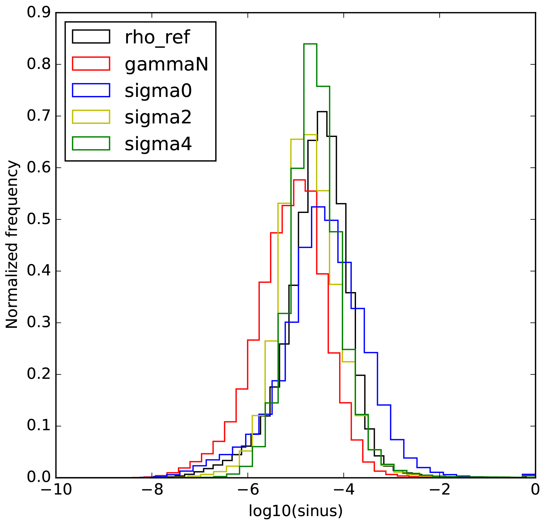
https://www.ocean-sci.net/15/21/2019/os-15-21-2019-f03

Figure 3Histogram of the decimal logarithm of the squared sine between the gradient of γ and the neutral vector d weighted by the volume of each point. log₁₀(sin²(∇γ,d)) for ρ_ref (black), γⁿ (red), σ₀ (blue), σ₂ (yellow) and σ₄ (green).

Download

ρ_ref, σ₂ and σ₄ give similar angles, with most of their values slightly larger than 10⁻⁵. γⁿ gives the smallest angles among the variables under consideration here, with most of its values smaller than 10⁻⁵, while σ₀ gives the largest, with a large number of points having values larger than 10⁻⁴. Altogether, these observations could suggest that the effective diffusivity of γⁿ should be the smallest overall, that the effective diffusivity of ρ_ref should be of the same order as that for σ₂ and σ₄, and that the effective diffusivity for σ₀ should be the largest of all. It is, however, hard to predict the values of the effective diffusivity coefficient for each density variable from Fig. 3, only since the small number of points with very large angle values (hardly visible in Fig. 3) could dominate the large number of points with small angles, and since the spatial variability of the isoneutral mixing coefficient could correlate with the spatial variability of the angle. We thus calculate the effective diffusivity coefficient using these angle values for each density variable.

Figure 4 shows the decimal logarithm of the effective diffusivity K_eff for the five variables as a function of the reference depth under two possible choices of K_i.

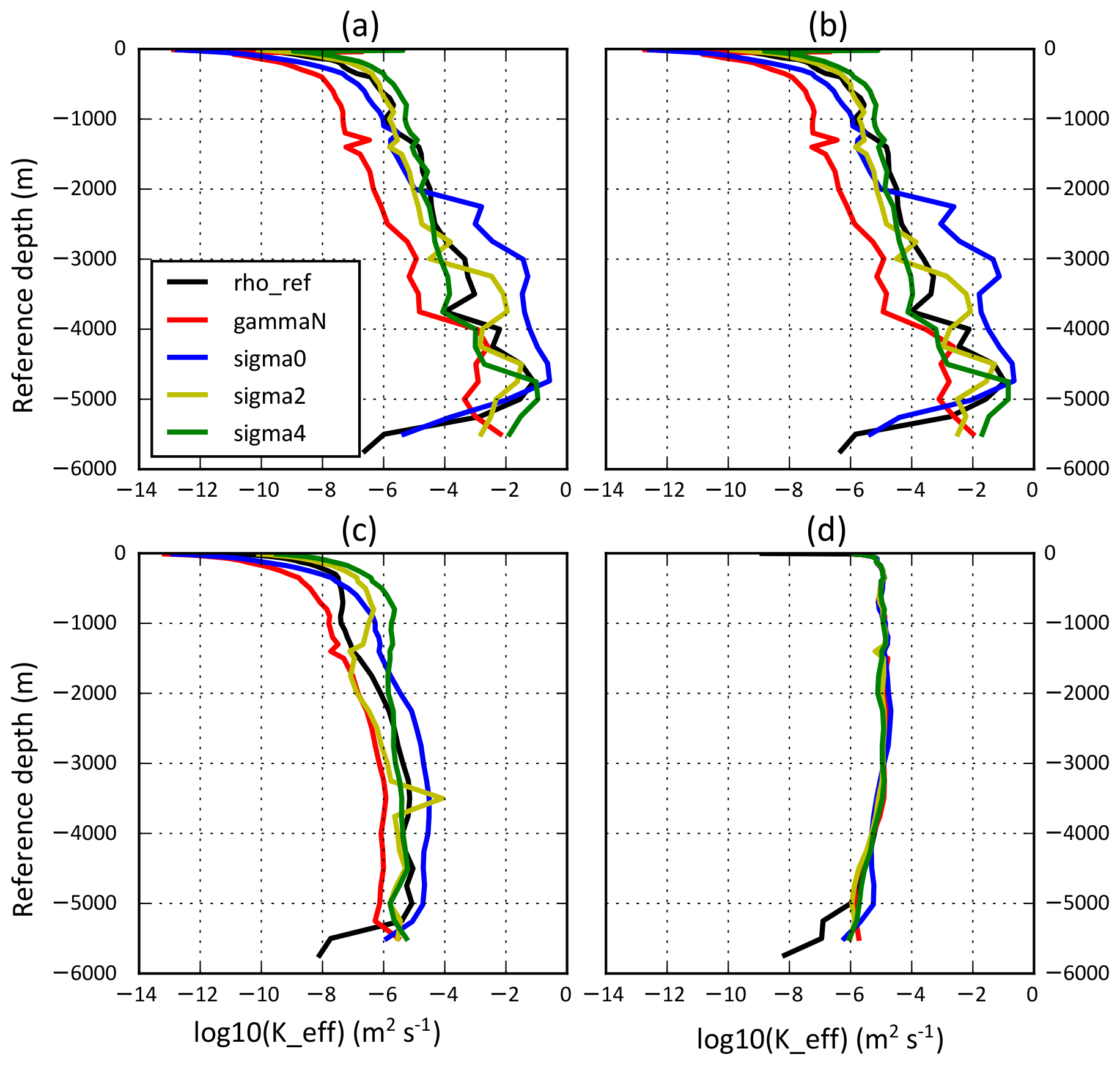
https://www.ocean-sci.net/15/21/2019/os-15-21-2019-f04

Figure 4log₁₀ of the effective diapycnal diffusivity coefficient K_eff as a function of the reference depth (meters; and as defined by Eq. 10) for ρ_ref (black), γⁿ (red), σ₀ (blue), σ₂ (yellow) and σ₄ (green). Panels (a), (b) and (c) correspond to a K_eff calculated with different isoneutral diffusivity coefficient. (a) K_iso=1000 m² s⁻¹; (b) variable isoneutral diffusivity coefficient given by Forget et al. (2015). (c) Same as (b), but without 5 % of the largest angles. (d) log₁₀K_eff calculated from a variable dianeutral diffusivity coefficient given by the inverse calculation of Forget et al. (2015).

Download

The first case (Fig. 4a) assumes a constant isoneutral coefficient: K_i=1000 m² s⁻¹. Under this assumption, for every density variable, K_eff increases, on average, with the reference depth, from values between 10⁻¹² and 10⁻⁸ m² s⁻¹ close to surface reference depth to values between 10⁻⁶ and 0 m² s⁻¹ at the deepest reference depths. This increase in K_eff reflects that the largest discrepancy between the neutral vector and the gradients of the five density variables are generally located in the Antarctic Circumpolar Current (ACC), where the highest densities, and thus deepest reference depths, outcrop (see below). K_eff for γⁿ and σ₀ are similar between −800 and 0 m depth, with values ranging from 10⁻⁸ m² s⁻¹ at the surface to 10⁻⁶ m² s⁻¹ at −800 m. σ₂, σ₄ and ρ_ref give values up to 100 times larger in the same depth range. Between −4000 and −800 m depth, γⁿ gives the smallest K_eff which is slowly increasing from 10⁻⁶ to 10⁻⁵ m² s⁻¹ as the depth decreases. In the same depths, ρ_ref, σ₀, σ₂ and σ₄ give values at least 10 times larger (up to 1000 times larger for σ₀ below −2000 m). Below −4000 m depth, all density variables have a K_eff larger than 10⁻⁴ m² s⁻¹. Note that 10⁻⁴ m² s⁻¹ is the widely cited canonical estimate of diapycnal mixing inferred from the global heat and mechanical energy budgets seen in Munk (1966) and Munk and Wunsch (1998). At the deepest levels, under −5000 m, σ₀ and ρ_ref have a smaller K_eff than γⁿ, suggesting that their local gradients are very nearly aligned with the neutral vector at these deep reference depths. The second case (Fig. 4b) assumes a spatially variable isoneutral coefficient given by the inverse calculation of Forget et al. (2015), which gives a three-dimensional distribution of K_i at about 1^∘ resolution for the global ocean. This database contains values ranging from 9000 m² s⁻¹ (in the Atlantic deep water formation zone at the surface, in western boundary currents and in the ACC) to values close to 0 (in the deep pelagic ocean). The estimated K_eff values for this choice are very close to those obtained under the previous assumption of constant diffusivity for all variables, showing the small sensitivity of our results to spatial variations of isoneutral diffusion, which is further discussed below.

To investigate the importance of the localised large departure from neutrality in the construction of K_eff, we removed 5 % of the largest non-neutral values of the angle for each reference surface (Fig. 4, panel c). Without 5 % of the largest values, K_eff is much smaller than the previous one for every density variable with values at every depth smaller than 10⁻⁴ m² s⁻¹. As before, the effective diffusivity increases rapidly when close to the surface and then more slowly below −1000 m (except at a few depths for σ₂ and σ₄ and at deep reference depths for ρ_ref and σ₀) with the reference depth for all density variables. γⁿ gives the smallest values for almost all reference depths, with values from 10⁻¹⁰ m² s⁻¹ close to the surface of the reference space to 10⁻⁶ m² s⁻¹ at the deepest levels. σ₂ gives the second smallest values for reference depths smaller than −1500 m but is overtaken by σ₀ and ρ_ref at larger depths. ρ_ref, σ₀, σ₂ and σ₄ all give effective diffusivities of the order of or larger than 10⁻⁵ m² s⁻¹ at some depths below −2000 m.

This calculation shows that the isoneutral contribution to effective diapycnal mixing is very localised spatially with 5 % of each surface accounting for most of the effective diffusivity for all the density variables under consideration here. However, even without this top 5 %, K_eff remains close to or above 10⁻⁵ m² s⁻¹ for all variables except γⁿ. Returning to the similarity between panels (a) and (b) in Fig. 4, the location of the top 5 % values are correlated with local K_i values (from the Forget et al., 2015, database) around 1000 m² s⁻¹ which therefore explain the lack of sensitivity of our results to the choice of K_i between (a) and (b). Panel (d) shows K_eff calculated using a dianeutral mixing coefficient given by Forget et al. (2015), where the inverse calculation assumes no isoneutral mixing. The formula for this calculation is obtained by replacing the sine by a cosine and K_i by K_d in formula (10), following formula (5), i.e.

\begin{matrix} (14) & K_{eff} (z_{r}) = \frac{\int_{z_{r} = const} K_{d} | \nabla z_{r} | \cos^{2} (\nabla z_{r}, d) d S}{A (z_{r})} . \end{matrix}

K_eff values are smaller or close to 10⁻⁵ m² s⁻¹ at all reference depths for all density variables. For reference depths deeper than 1000 m, these values are much smaller than the effective diffusivity estimated from the isoneutral mixing coefficient as shown in panel (a) or (b). Without the 5 % of the largest values on each density surface, K_eff estimated from variable K_i (Fig. 4c) is smaller than the one estimated from variable K_d for all density variables above 1000 m. The exception is γⁿ, which gives the K_eff estimated from K_i approximately 10 times smaller than K_eff from K_d at all reference depths below 1000 m. The values obtained from the dianeutral coefficient are much less sensitive to the choice of density variable than the values obtained from the isoneutral mixing coefficient, because for small angles, $\cos^{2} (\nabla z_{r}, d) \approx 1 - (\nabla z_{r}, d)^{2}$ depends on the angle only at second order.

https://www.ocean-sci.net/15/21/2019/os-15-21-2019-f05

Figure 5Decimal logarithm of the sine between the neutral vector, and the gradient of ρ_ref (a), γⁿ (b) and σ₀ (c) as a function of latitude and depth at 30^∘ W (in the Atlantic).

Download

The largest angles between the neutral vector and the gradient of the density variable are found mostly in the ACC at all depths for ρ_ref and γⁿ and at all depths for σ₀, as illustrated in Fig. 5. This suggests that, in this region, all the density variables studied above introduce significant biases to the estimation of diapycnal mixing.

4 Conclusions

Mixing of heat and salt in numerical ocean models is commonly parameterised by means of a neutral rotated diffusion tensor using the dianeutral and isoneutral mixing coefficients K_d and K_i relating to density surfaces that are only defined locally. In contrast, inverse methods based on Walin-type water mass analyses produce observationally constrained diapycnal diffusivities K_γ for the globally defined density variable γ underlying the isopycnal analysis. Since inverse methods give us information about K_γ, while what we need in numerical ocean models is K_d, our ability to use Walin-type inverse approaches to constrain neutral rotated diffusion tensors therefore depends on our ability to understand how the various diffusivities K_γ and K_d are interrelated.

In this paper, we have presented a new framework for assessing the contribution of isoneutral diffusion to the effective diapycnal mixing coefficient K_eff for five different density variables, chosen for their widespread use in the oceanographic community, namely γⁿ, ρ_ref, σ₀, σ₂ and σ₄. Our results reveal that the contribution of isoneutral mixing to the effective diapycnal mixing experienced by each density variable can be as large as 10⁻⁴ and up to 0.1 m² s⁻¹ for reference depths deeper than 2000 m. These values are typically 10 to 100 times larger below −1000 m and up to 1000 times larger below −4000 m than estimations for the effective diapycnal mixing due to the dianeutral mixing alone (which are around or below 10⁻⁵ m² s⁻¹). As expected, γⁿ, constructed to be as neutral as practically feasible, is the least affected by isoneutral diffusion of all density variables considered. Nevertheless, it still appears to experience values larger than 10⁻⁴ m² s⁻¹ for reference depths below −4000 m. These values are 10 to 100 times larger than the corresponding effective mixing due to the direct effect of a (variable) dianeutral mixing coefficient. Note that an added difficulty pertaining to the use of γⁿ stems from its non-material character. As a result, the validity of defining an effective diapycnal diffusivity for γⁿ using the present approach depends on such non-material effects to be small, or at least much smaller than the contribution from isopycnal diffusion discussed here, which is difficult to evaluate.

Our results thus suggest that the potential contamination due to isoneutral mixing should always be assessed for any inference of diapycnal mixing based on the use of any density variable γ(S,θ), in Walin-like water mass analysis, for instance. In agreement with previous studies (McDougall and Jackett, 2005), the regions of large discrepancy between the neutral vector and the gradient of each surface are localised in space and mainly confined to the deep Southern Ocean. However, while representing a very small amount of volume of the ocean, these discrepancies are important in setting the effective diffusivity values. Indeed, without 5 % of the largest angle values between the neutral vector and the local γ gradient, all variables give an effective diapycnal mixing smaller than 10⁻⁴ m² s⁻¹. Moreover, the estimated values everywhere are comparable to or smaller than the effective mixing estimated from dianeutral mixing only. Note that, even after removal of the largest angles, isoneutral and dianeutral mixing equally contribute to the effective diapycnal mixing. In the context of inverse methods, this still represents a potential uncertainty of up to a factor of 2 in the estimation of diapycnal mixing due to the contamination by isoneutral mixing. The concentration of discrepancies is even stronger for γⁿ, since the effective diffusivity coefficient after the removal of the 5 % of the largest values decreases below 10⁻⁶ m² s⁻¹. This is a contamination of only 10 % for the typical diapycnal mixing values of 10⁻⁵ m² s⁻¹ found in the thermocline and abyssal plains (Ledwell et al., 1998) and is much less for enhanced mixing values found above rough topography (Polzin et al., 1997).

Overall, the K_eff profiles for each density variable become similar without the 5 %, suggesting that the choice of the density variable is less important when the Southern Ocean is not taken into account. However, when no part of the ocean is removed (as in the case of a type of calculation like Walin, 1982, for instance), the effective diffusivities found in this article are very sensitive to the density variable under consideration. This is at odds with the results of Megann (2018) and could suggest that their effective diffusivities are mainly driven by spurious numerical mixing.

Our results show that the evaluation of effective diapycnal mixing using a sorting algorithm of density (Griffies et al., 2000; Hill et al., 2012; Ilıcak et al., 2012), which amounts to diagnosing the diapycnal flux through ρ_ref, is likely to be significantly contaminated by isoneutral diffusion owing to the large departure from the neutrality of ρ_ref in the polar regions if a nonlinear equation of state is used (which is not the case in the studies cited above). Note that this is a distinct effect from the density sinks and sources due to the nonlinear equation of state influencing the time variation of the reference density (see Eq. 11), which are also a source of contamination of the diapycnal flux from the isoneutral diffusion when using a sorting algorithm. It follows that diagnosing the spurious diapycnal mixing resulting from numerical advection schemes for a nonlinear equation of state remains an outstanding challenge and that progress related to this topic must take into account the theoretical considerations developed here.

This work advocates for the construction of a density function γ(θ,S) that would minimize the influence of isoneutral mixing on the effective diapycnal diffusivity coefficient. As shown by Tailleux (2016), so far the best material density variable is a function of Lorenz reference density, but it appears theoretically possible to construct an even more neutral one. Whether the ω surfaces of Klocker et al. (2009) can be used for global inversions is unclear, because their improved neutrality might be achieved at the expense of materiality, which remains to be quantified.

Data availability

The World Ocean Atlas dataset used in this study is available on the NOAA website: https://www.nodc.noaa.gov (Gouretski and Koltermann, 2004).

Appendix A

A conceptual difficulty in the ocean is the impossibility of constructing a mathematically well-defined materially conserved variable γ(S,θ) allowing us to write N=C₀∇γ with C₀ as an integrating factor. In the spatial domain, this can be attributed mathematically to the non-zero helicity of N (see McDougall and Jackett, 1988 a). More instructive and illuminating, however, is proving the result directly in thermohaline space. To that end, let us assume that such a variable $γ = γ (S, θ)$ exists and show that it leads to a contradiction. To that end, let us perform a change of variables from (S,θ) space to (γ,θ) space, similarly to Tailleux (2016). Let us denote this $J = \partial (γ, θ) / \partial (S, θ)$ , the Jacobian of the transformation. It is easy to see that $J = \partial γ / \partial S$ , which we assume to be non-zero so that the transformation is invertible. This makes it possible to regard $S = \hat{S} (γ, θ)$ as a function of γ and θ. Likewise, we can define $ρ = ρ (S, θ) = ρ (\hat{S} (γ, S), θ) = \hat{ρ} (γ, S)$ , where the hat notation refers to the variables viewed as functions of γ and θ instead of S and θ. As a result, the neutral vector can be equivalently written as

\begin{array}{l} N & = - \frac{g}{ρ} (\frac{\partial ρ}{\partial S} \nabla S + \frac{\partial ρ}{\partial θ} \nabla θ) = \\ (A1) & - \frac{g}{ρ} (\frac{\partial \hat{ρ}}{\partial γ} \nabla γ + \frac{\partial \hat{ρ}}{\partial θ} \nabla θ) . \end{array}

In order for N to align with ∇γ, one would need the quantity $\partial \hat{ρ} / \partial θ$ to vanish. An expression for $\partial \hat{ρ} / \partial θ$ can be obtained using the following series of identities:

\begin{matrix} (A2) & \frac{\partial \hat{ρ}}{\partial θ} = \frac{\partial (\hat{ρ}, γ)}{\partial (θ, γ)} = \frac{\partial (ρ, γ)}{\partial (S, θ)} \frac{\partial (S, θ)}{\partial (θ, γ)} = \frac{1}{J} \frac{\partial (γ, ρ)}{\partial (S, θ)}, \end{matrix}

where we used the usual properties of Jacobian operators, including composition and anti-symmetry. Equation (A2) shows that for $\partial \hat{ρ} / \partial θ = J^{- 1} \partial (γ, ρ) / \partial (S, θ)$ to be zero, this would require ρ to be a function of γ(S,θ) alone, but this cannot be true, because ρ also depends on pressure.

Calculation of K_eff

The following steps describe the calculation of the effective diffusivity coefficient for a given γ(S,θ) in detail:

The reference depth z_r(S,θ) is calculated following formula (7), and its gradient $| \nabla z_{r} |$ is then computed everywhere.
The neutral vector is calculated as the gradient of the locally referenced potential density.
The sinus of the angle between ∇z_r and d, sin(∇z_r,d), is calculated using the cross product between ∇z_r and d:
$\begin{matrix} (B1) & | \sin (\nabla z_{r}, d) | = \frac{| \nabla z_{r} \times d |}{| \nabla z_{r} |}, \end{matrix}$
where × is the cross product and d the normalised neutral vector $d = N / | N |$ .
The product $K_{i} | \nabla z_{r} | \sin^{2} (\nabla z_{r})$ is interpolated to and integrated with $z_{r} (S, θ) = const .$ surfaces.
K_eff is then equal to the integral obtained at the previous step divided by the area of the ocean at depth z_r, i.e. A(z_r).

Appendix C: Equation (11)

The evolution equation for γ is:

\begin{array}{l} \frac{d γ}{d t} & = \frac{\partial γ}{\partial θ} \frac{d θ}{d t} + \frac{\partial γ}{\partial S} \frac{d S}{d t} = \frac{\partial γ}{\partial θ} \nabla (K \nabla θ) \\ (C1) & + \frac{\partial γ}{\partial S} \nabla (K \nabla S) + \frac{\partial γ}{\partial θ} f_{θ} + \frac{\partial γ}{\partial S} f_{S} \\ = \nabla (K \nabla γ) - K \nabla θ \cdot \nabla (\frac{\partial γ}{\partial θ}) \\ (C2) & - K \nabla S \cdot \nabla (\frac{\partial γ}{\partial S}) + f_{γ}, \end{array}

where f_θ and f_S are the surface heat and haline fluxes and where $f_{γ} = \frac{\partial γ}{\partial θ} f_{θ} + \frac{\partial γ}{\partial S} f_{S}$ . Then let z_r(X,t) be the reference level of γ defined by Eq. (7) so that γ can now be written as $γ (S, θ) = γ_{r} (z_{r}, t)$ . Then, integrating Eq. (C2) on a volume V(z_r) defined by water parcels of a reference level larger than or equal to z_r gives

\begin{array}{l} \int_{V (z_{r})} \frac{\partial γ}{\partial t} d V + γ_{r} (z_{r}, t) \int_{z_{r} = const} u \cdot n d S = \int_{z_{r} = const} K \nabla γ \cdot n d S \\ - \int_{V (z_{r})} K \nabla θ \cdot \nabla (\frac{\partial γ}{\partial θ}) + K \nabla S \\ (C3) & \cdot \nabla (\frac{\partial γ}{\partial S}) d V + \int_{V (z_{r})} f_{γ} d V, \end{array}

where z_r=const refers to the constant z_r surface. $n = \frac{\nabla γ}{| \nabla γ |} = - \frac{\nabla z_{r}}{| \nabla z_{r} |}$ is the local normal to the surface γ=const, and the minus sign arises because the integration is done toward deeper values of z_r. The second term on the left-hand side is zero because of the non-divergence of the velocity, and the first term can be written as

\begin{matrix} (C4) & \int_{V (z_{r})} \frac{\partial γ}{\partial t} d V = \frac{\partial}{\partial t} \int_{V (z_{r})} γ_{r} d V^{'} - γ_{r} \underset{= 0}{\underset{︸}{\frac{\partial V (z_{r})}{\partial t}}} . \end{matrix}

The second term on the right-hand side is zero, because the total volume at constant z_r is independent of time (see formula 7). Using Eq. (C4) and the z_r derivative of Eq. (C3) we get

\begin{matrix} (C5) & \frac{\partial γ_{r}}{\partial t} = \frac{1}{A (z_{r})} \frac{\partial}{\partial z_{r}} (A (z_{r}) K_{eff} (z_{r}) \frac{\partial γ_{r}}{\partial z_{r}}) + NL + forcing, \end{matrix}

where we have used formula (7) and the fact that the volume integral of a function of only z_r can be expressed as an integral over the reference depth

\begin{array}{l} \frac{\partial}{\partial z_{r}} (\frac{\partial}{\partial t} \int_{V (z_{r})} γ_{r} d V^{'}) = \frac{\partial}{\partial t} (\frac{\partial}{\partial z_{r}} \int_{z_{r}}^{0} A (z_{r}^{'}) γ_{r} (z_{r}^{'}, t) d z_{r}^{'}) = \\ (C6) & - A (z_{r}) \frac{\partial γ_{r}}{\partial t}, \end{array}

and where

\begin{array}{l} NL & = \frac{1}{A (z_{r})} \frac{\partial}{\partial z_{r}} \\ (C7) & (\int_{V (z_{r})} (K \nabla θ \cdot \nabla (\frac{\partial γ}{\partial θ}) + K \nabla S \cdot \nabla (\frac{\partial γ}{\partial S})) d V), \end{array}

\begin{matrix} (C8) & forcing = - \frac{1}{A (z_{r})} \frac{\partial}{\partial z_{r}} (\int_{V (z_{r})} f_{γ} d V), \end{matrix}

and, finally, K_eff is given by formula (10).

Competing interests

The authors declare that they have no conflict of interest.

Acknowledgements

This work was supported by the grant NE/K016083/1 “Improving simple climate models through a traceable and process-based analysis of ocean heat uptake (INSPECT)” and its follow-up NE/R010536/1 “New prOcess-based UndersTanding of ocean heat Uptake with an application to improved Climate pRojections for pOlicy and Planning” (OUTCROP) of the UK Natural Environment Research Council (NERC). Modeling results presented in this study are available upon request to the corresponding author.

Edited by: Eric J. M. Delhez
Reviewed by: Sjoerd Groeskamp and two anonymous referees

References

de Boyer Montégut, C., Madec, G., Fischer, A. S., Lazar, A., and Iudicone, D.: Mixed layer depth over the global ocean: An examination of profile data and a profile-based climatology, J. Geophys. Res.-Oceans, 109, https://doi.org/10.1029/2004JC002378, 2004. a

Forget, G., Ferreira, D., and Liang, X.: On the observability of turbulent transport rates by Argo: supporting evidence from an inversion experiment, Ocean Sci., 11, 839–853, https://doi.org/10.5194/os-11-839-2015, 2015. a, b, c, d, e

Gnanadesikan, A., Pradal, M.-A., and Abernathey, R.: Isopycnal mixing by mesoscale eddies significantly impacts oceanic anthropogenic carbon uptake, Geophys. Res. Lett., 42, 4249–4255, 2015. a

Gouretski, V. and Koltermann, K. P.: WOCE global hydrographic climatology, Berichte des BSH, 35, 1–52, 2004 (data available at: https://www.nodc.noaa.gov, last access: 1 July 2018). a, b

Griffies, S. M., Pacanowski, R. C., and Hallberg, R. W.: Spurious diapycnal mixing associated with advection in az-coordinate ocean model, Mon. Weather Rev., 128, 538–564, 2000. a, b, c

Hill, C., Ferreira, D., Campin, J.-M., Marshall, J., Abernathey, R., and Barrier, N.: Controlling spurious diapycnal mixing in eddy-resolving height-coordinate ocean models–Insights from virtual deliberate tracer release experiments, Ocean Model., 45, 14–26, 2012. a

Huber, M., Tailleux, R., Ferreira, D., Kuhlbrodt, T., and Gregory, J.: A traceable physical calibration of the vertical advection-diffusion equation for modeling ocean heat uptake, Geophys. Res. Lett., 42, 2333–2341, https://doi.org/10.1002/2015gl063383, 2015. a

Ilıcak, M., Adcroft, A. J., Griffies, S. M., and Hallberg, R. W.: Spurious dianeutral mixing and the role of momentum closure, Ocean Model., 45, 37–58, 2012. a, b

Iselin, C. O.: The influence of vertical and lateral turbulence on the characteristics of the waters at mid-depths, EOS T. Am. Geophys. Un., 20, 414–417, 1939. a

Jackett, D. R. and McDougall, T. J.: A neutral density variable for the world's oceans, J. Phys. Oceanogr., 27, 237–263, https://doi.org/10.1175/1520-0485(1997)027<0237:andvft>2.0.co;2, 279, 1997. a, b, c, d

Klocker, A. and McDougall, T. J.: Influence of the Nonlinear Equation of State on Global Estimates of Dianeutral Advection and Diffusion, J. Phys. Oceanogr., 40, 1690–1709, https://doi.org/10.1175/2010jpo4303.1, 2010. a

Klocker, A., McDougall, T. J., and Jackett, D. R.: A new method for forming approximately neutral surfaces, Ocean Sci., 5, 155–172, https://doi.org/10.5194/os-5-155-2009, 2009. a, b

Kuhlbrodt, T. and Gregory, J.: Ocean heat uptake and its consequences for the magnitude of sea level rise and climate change, Geophys. Res. Lett., 39, https://doi.org/10.1029/2012GL052952, 2012. a

Ledwell, J. R., Watson, A. J., and Law, C. S.: Mixing of a tracer in the pycnocline, J. Geophys. Res.-Oceans, 103, 21499–21529, 1998. a

Lee, M.-M., Coward, A. C., and Nurser, A. G.: Spurious diapycnal mixing of the deep waters in an eddy-permitting global ocean model, J. Phys. Oceanogr., 32, 1522–1535, 2002. a, b, c

Lumpkin, R. and Speer, K.: Global ocean meridional overturning, J. Phys. Oceanogr., 37, 2550–2562, 2007. a

McDougall, T. J.: thermobaricity, cabbeling, and water-mass conversion, J. Geophys. Res.-Oceans, 92, 5448–5464, https://doi.org/10.1029/JC092iC05p05448, 134, 1987. a

McDougall, T. J. and Jackett, D. R.: On the helical nature of neutral trajectories in the ocean, Prog. Oceanogr., 20, 153–183, https://doi.org/10.1016/0079-6611(88)90001-8, 26, 1988a. a

McDougall, T. J. and Jackett, D. R.: On the helical nature of neutral trajectories in the ocean, Prog. Oceanogr., 20, 153–183, 1988b. a

McDougall, T. J. and Jackett, D. R.: An assessment of orthobaric density in the global ocean, J. Phys. Oceanogr., 35, 2054–2075, 2005. a, b, c, d

McDougall, T. J., Groeskamp, S., and Griffies, S. M.: On geometrical aspects of interior ocean mixing, J. Phys. Oceanogr., 44, 2164–2175, 2014. a

Megann, A.: Estimating the numerical diapycnal mixing in an eddy-permitting ocean model, Ocean Model., 121, 19–33, https://doi.org/10.1016/j.ocemod.2017.11.001, 2018. a, b

Montgomery, R.: The present evidence on the importance of lateral mixing processes in the ocean, B. Am. Meteorol. Soc., 21, 87–94, 1940. a

Munk, W. and Wunsch, C.: Abyssal recipes II: energetics of tidal and wind mixing, Deep-Sea Res. Pt. I, 45, 1977–2010, https://doi.org/10.1016/s0967-0637(98)00070-3, 1998. a

Munk, W. H.: Abyssal recipes, in: Deep Sea Research and Oceanographic Abstracts, 13, 707–730, Elsevier, 1966. a

Nurser, A. J. G., Marsh, R., and Williams, R. G.: Diagnosing water mass formation from air-sea fluxes and surface mixing, J. Phys. Oceanogr., 29, 1468–1487, https://doi.org/10.1175/1520-0485(1999)029<1468:dwmffa>2.0.co;2, 1999. a

Polzin, K. L., Toole, J. M., Ledwell, J. R., and Schmitt, R. W.: Spatial variability of turbulent mixing in the abyssal ocean, Science, 276, 93–96, https://doi.org/10.1126/science.276.5309.93, 1997. a

Pradal, M.-A. and Gnanadesikan, A.: How does the Redi parameter for mesoscale mixing impact global climate in an Earth system model?, J. Adv. Model. Earth Sy., 6, 586–601, 2014. a

Redi, M. H.: Oceanic isopycnal mixing by coordinate rotation, J. Phys. Oceanogr., 12, 1154–1158, 1982. a, b

Saenz, J. A., Tailleux, R., Butler, E. D., Hughes, G. O., and Oliver, K. I. C.: Estimating Lorenz's Reference State in an Ocean with a Nonlinear Equation of State for Seawater, J. Phys. Oceanogr., 45, 1242–1257, https://doi.org/10.1175/jpo-d-14-0105.1, 2015. a, b, c

Solomon, H.: On the representation of isentropic mixing in ocean circulation models, J. Phys. Oceanogr., 1, 233–234, 1971. a

Speer, K. G.: A note on average cross-isopycnal mixing in the North Atlantic ocean, Deep-Sea Res. Pt. I, 44, 1981–1990, https://doi.org/10.1016/s0967-0637(97)00054-x, 1997. a, b

Tailleux, R.: Neutrality Versus Materiality: A Thermodynamic Theory of Neutral Surfaces, Fluids, 1, 32, https://doi.org/10.3390/fluids1040032, 2016. a, b

Urakawa, L., Saenz, J., and Hogg, A.: Available potential energy gain from mixing due to the nonlinearity of the equation of state in a global ocean model, Geophys. Res. Lett., 40, 2224–2228, 2013. a

Walin, G.: On the relation between sea-surface heat flow and thermal circulation in the ocean, Tellus, 34, 187–195, 180, 1982. a

Winters, K. B. and D'Asaro, E. A.: Diascalar flux and the rate of fluid mixing, J. Fluid Mech., 317, 179–193, 1996. a, b

We assume fixed composition, thus allowing one to treat practical (conductivity) salinity and Absolute Salinity as equivalent, since the two are then linked to each other by a fixed conversion factor. Note that all the arguments could be reformulated using the more recent conservative temperature Θ if desired without changing the conclusions.