2.1 Satellite altimetry

We use two altimetry missions with distinct characteristics: Jason-2 and SARAL/AltiKa. Jason-2 was launched in June 2008 and provides long time series of data with a 10-day repeat observation cycle. The performance of SARAL is significantly better. With a better signal-to-noise ratio, it resolves smaller spatial scales than Jason-2: ∼40 km against ∼50 km (Dufau et al., 2016; Verron et al., 2018). However, the corresponding time series started only in February 2013 and have a 35-day repeat observation cycle, so they are a priori not really adapted to the monitoring of coastal ocean variability. On the other hand, the SARAL orbit leads to a smaller distance between tracks compared to Jason-2 (Fig. 1). Here we focus only on the SARAL tracks 302, 343 and 887 and on the Jason-2 track 222, providing the closest data from the in situ observations.

For both missions, because it is one of the most often used in coastal altimetry applications, we first used the X-TRACK regional product from the CTOH (https://doi.org/10.6096/CTOH_X-TRACK_2017_02, Birol et al., 2017b), processed with a coastal-oriented strategy (Birol et al., 2017a). It consists of time series of 1 Hz sea level anomalies (SLAs) every 6–7 km along the satellite tracks, available from 20 July 2008 to 1 October 2016 for Jason-2 (i.e., 300 cycles) and from 24 March 2013 to 12 June 2016 for SARAL (i.e., 34  cycles). In order to evaluate the skill of the 20 and 40 Hz altimetry measurements of the Jason-2–SARAL altimeters for circulation studies relative to the conventional 1 Hz data, we have also used an experimental high-rate version of these datasets provided by the CTOH (Sect. 3.4). The processing is the same as for 1 Hz SLA, except that the high-rate SLAs are computed from the 20–40 Hz range data provided in the AVISO L2 products (https://www.aviso.altimetry.fr/fileadmin/documents/data/tools/hdbk_j2.pdf, last access: 14 November 2018, and https://www.aviso.altimetry.fr/fileadmin/documents/data/tools/SARAL_Altika_products_handbook.pdf, last access: 14 November 2018). The resulting sea level time series are available every ∼0.29 and ∼0.19 km along the satellite tracks for Jason-2 and SARAL, respectively. However, we must keep in mind that if the use of high-rate altimeter measurements allows us to significantly improve the spatial resolution, the resulting SLAs are much noisier (see, for example, Birol and Delebecque, 2014). Considering the data availability (see below for the in situ observations), the study period chosen is 2010–2016 for all altimetry datasets.

The Jason-2 altimeter is designed as “conventional altimetry” as it operates in the Ku-band frequency. The SARAL altimeter operates in the Ka-band, allowing for a better performance in terms of spatial resolution (the radar footprint is smaller) and measurement noise. Morrow et al. (2017) analyzed the “mesoscale capability” (defined as the wavelength at which the noise is larger than the signal, which varies spatially as shown by Dufau et al., 2016) of these two altimeters in the NWMed using a statistical method (Xu and Fu, 2012). It allows us to have an estimate of the size of the structures that can be theoretically detected by each altimeter (on average) and to define the optimal data spatial filtering. Here, we did the same computation for each of the four tracks used in this study using all the data available, unlike in Morrow et al. (2017) in which the data located over the continental shelf were discarded. We obtained 49 km for the SARAL track 302, 39 km for the SARAL track 343, 34 km for the SARAL track 887 and 67 km for the Jason-2 track 222, which is coherent with the results of Morrow et al. (2017), who obtained 39 km for SARAL and 55 km for Jason-2 without the coastal altimetry observations. It suggests that the quality of nearshore altimetry SLA remains good. The lower values obtained for SARAL are due to the better signal-to-noise ratio of the AltiKa altimeter compared to Jason-2. The differences found among the three SARAL tracks are explained by their respective geographical locations. They capture different mesoscale features.

In order to have the best signal-to-noise ratio, we then filtered the data with a low-pass Loess filter using a cutoff frequency of 35 km for SARAL. Note that we have chosen a single value for the different SARAL tracks in order to have the same data processing and facilitate comparison between the different datasets. For Jason-2, we chose to use a processing as close as possible to the one of SARAL and then used a cutoff frequency of 40 km. The same low-pass filters were used for both 1 Hz and high-rate SLAs. One needs to keep in mind that noise remains in the filtered Jason-2 data.

Altimetry only provides sea level anomalies relative to a temporal mean. In order to estimate currents as close as possible to the currents measured or derived from the other instruments (see below), we added the regional mean dynamic topography (MDT) from Rio et al. (2014) to the altimetric SLA and computed the surface velocities (u) from the total sea level gradients observed between consecutive points along the track, assuming that the fluid is in geostrophic balance:

where f is the Coriolis parameter, g the gravitational constant and Δx the distance between the points.

Only the across-track component of the geostrophic currents can be derived. The MDT product used is a regional product with a horizontal resolution of 1∕16^∘ (i.e., lower than altimetry resolution in the along-track direction). Compared to other MDT products, it allows for a better representation of the NC in the Ligurian Sea (Rio et al., 2014).

2.2 In situ measurements

2.2.1 Glider data

Gliders have been deployed in the NWMed since 2005. However, it is only since 2009 that they have been regularly operating as part of the MOOSE network (http://www.moose-network.fr/?page_id=272, last access: 20 November 2018). In particular, on the Nice–Calvi line (Fig. 1, pink line), 36 deployments were undertaken between 2009 and 2016. Some of them have already been analyzed in different studies with different scientific objectives (Piterbarg et al., 2014, focused on frontal variability; Bosse et al., 2015, investigated sub-mesoscale anticyclones; Niewiadomska et al., 2008, analyzed physical–biogeochemical coupling mechanisms). Each glider deployment encompasses several transects, and the database includes 204 sections; 192 of them are between 2010 and 2016. The ones that are too short (<60 km) or moving too far away (>15 km) from an average trajectory computed from the individual ones were discarded. Finally, 173 glider transects along this line were used in this study. It represents a huge amount of observations and a large number of cases available for comparisons with altimetry or with other in situ observations.

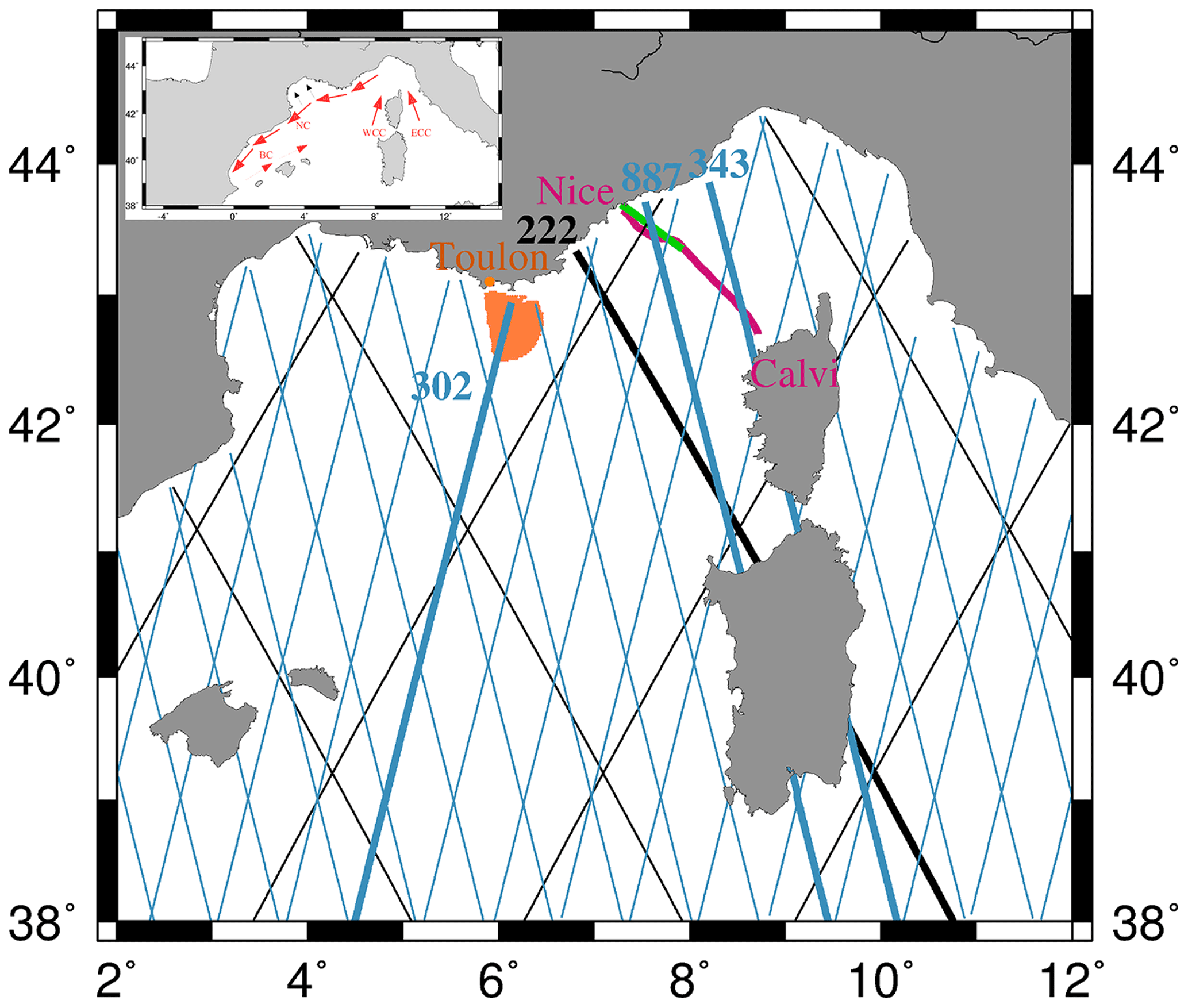
Figure 1Study area and data distribution. Jason-2 and SARAL tracks are represented by the black and blue lines, respectively. The satellite tracks used in the study are indicated in bold. The region in orange corresponds to the HF radar coverage. The Nice–Calvi glider line is in purple and the TETHYS ADCP transect is in green. A map of the schematic regional circulation is presented in the upper left corner.

Download

The campaigns were sliced into ascending (from Calvi to Nice) and descending (from Nice to Calvi) transects and the data were projected on a reference track. We assume that one dive or one ascent represents one vertical profile. In practice, data were discarded when the latitude was not monotonically varying or when the angular deviation between two consecutive points and the mean direction of the reference track was too strong (i.e., larger than 3 standard deviations (SDs) away from the mean angle). Then the data were gridded with a 4 km horizontal bin size along the reference track; 4 km corresponds to the average distance between two successive profiles.

During their mission, gliders measure temperature and salinity from the surface down to 1000 m (less if the bottom is shallower or if commanded to dive shallower). To avoid noise that is mainly due to aliased internal waves, temperature and salinity data have to be filtered. A Butterworth filter of second order (Durand et al., 2017) was applied. Different cutoff frequencies have been tested and we finally chose 15 km to avoid noise without removing small-scale variations (as in Bosse et al., 2017). From the temperature and salinity data we computed the density and then the geostrophic velocity component perpendicular to the reference track using the thermal wind equation. These velocities are referenced to 500 m, corresponding to the depth reached by all gliders. The difference with altimetry-derived currents is then that the barotropic component and the baroclinic component below 500 m are missing.

2.2.3 HF radars

The HF radar data used here (orange zone in Fig. 1) are also part of the MOOSE network (Zakardjian and Quentin, 2018). They target the area off the coast of Toulon as a key zone conditioning the behavior of the NC just upstream of the Gulf of Lions. Due to a sharp bathymetry and several islands that deflect the NC southwestward, significant mesoscale variability and cross-shelf exchanges exist in this area (Guihou et al., 2013), correlated with strong northwesterly winds (Mistral, Tramontane). The system consists of two HF (16 MHz) Wellen radar (WERA) instruments installed near Toulon in monostatic (Cap Sicié station) and bistatic (Cap Bénat–Porquerolles island stations) eight-antenna configurations (see Quentin et al., 2013, 2014, for details). They work with a 50 kHz bandwidth, resulting in a 3 km range resolution, a direction-finding method based on MUSIC (multiple-signal classification algorithm; see Lipa et al., 2006; Molcard et al., 2009) allowing for a 2^∘ azimuthal resolution and a time integration of 20 min. The radial velocity maps are averaged over a 1 h time window and Cartesian total velocities are then reconstructed on a regular 2×2 km grid. More details on this HF radar site can be found in Sentchev et al. (2017), who found an overall good agreement between derived radial velocities and in situ ADCP, with relative errors of 1 and 9 % and root mean square (RMS) differences of 0.02 and 0.04 m s⁻¹; this is slightly increased in velocity and direction for the reconstructed total velocities, but mainly in conditions of nonstationary wind forcing. The MOOSE HF radar database used here is made up of daily (one diurnal lunar period of 25 h) averaged surface currents computed from the reprocessed hourly total velocity data (QC level L3B, i.e., velocity threshold and geometric dilution of precision – GDOP – tests passed) with additional cleaning of residual RFI (radio frequency interference) outliers using an outlier removal algorithm based on the number of L3B valid data, variance and mean over an inertial period window (17 h at 43^∘ N). The data are then filtered from tides and inertial oscillations. The time series starts in May 2012 and ends in September 2014 with a total of 732 days of available data. The size of the area covered by total velocities after the GDOP test is roughly 60×40 km and it is located about 170 km westward of the glider and ADCP observations.

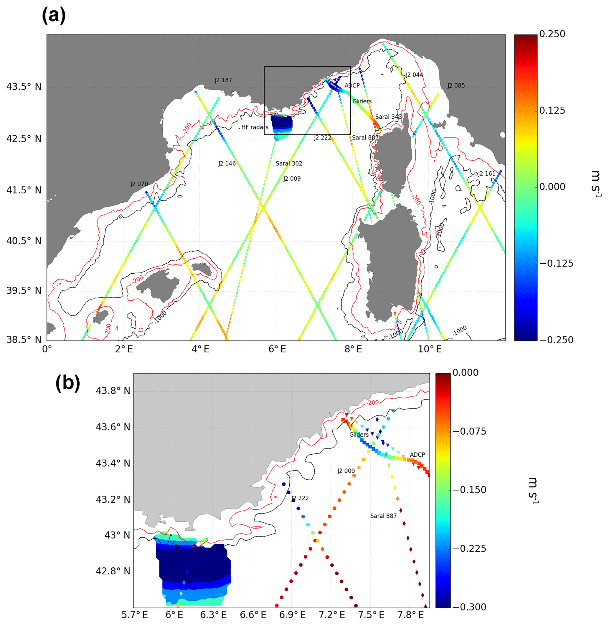
Figure 2(a) Map of the mean current values derived from ADCP, glider, HF radar and altimetry data over the period March 2013–October 2014. (b) Zoomed-in view of the northern Ligurian Sea (black rectangle indicated in panel a); 200 m (red line) and 1000 m (black line) isobaths are also shown. Current values are positive (negative) to the right (left) of the ship, glider or satellite tracks.

Download

2.3 Differences between the currents derived from the different observational techniques

In this study, we extensively compare the currents derived from the four different techniques described above with the objective of better understanding how they can optimally complement each other for the observation and study of variability in the NC circulation system. However, we must first have in mind the intrinsic characteristics of each type of current observation and the differences between the datasets.

2.3.1 Spatial and temporal sampling

First, the locations of the different types of observations do not coincide with each other, and their temporal and spatial sampling is also very different. After processing, current values are obtained every 2 km along the ship ADCP track, every 4 km along the glider line, in a 3 km resolution grid for the HF radar, every 5–6 to 7–8 km along the satellite track for 1 Hz Jason-2–SARAL altimetry and every 0.29 to 0.19 km for HF Jason-2–SARAL altimetry. Moreover, each instrument is characterized by specific measurement errors and a specific signal-to-noise ratio. Filtering has to be applied on the glider and altimetry data, still limiting the wavelengths of the current that can be resolved (see above and in Table 1). We also have to keep in mind instrumental limitations concerning the area that can be monitored. The ship ADCPs, the HF radars and the gliders have a higher spatial resolution than the filtered altimetry data but a much more limited spatial coverage. We also have to consider the fact that access to altimetry data, at least in the standard 1 Hz version, still remains limited in the 10–15 km coastal band. As the NC fluctuates in both location and width and at both seasonal and much higher frequencies (Albérola et al., 1995), it can make a large difference in the ability of the instrument considered to capture this current flowing along the continental slope, often located very close to the coastline (Fig. 2).

Table 1Main characteristics of the different current datasets used in this study.

Download Print Version | Download XLSX

Table 2Number of data samples per month for each current dataset during the period 1 January 2010–31 December 2016. The number of data selected for the climatology computation is indicated in brackets.

Download Print Version | Download XLSX

Concerning the temporal sampling, the HF radars and the altimetry provide current observations at regular intervals: every day for the HF radar product used here, every 10 days for Jason-2 and every 35 days for SARAL. The glider and ADCP data are available between zero and nine times per month and between zero and five times per month, respectively. These unevenly spaced time series make the corresponding data analysis more complex since it can produce significant biases in the distribution of the NC properties (for example, its seasonal variations; see Table 2). It will also be influenced by the period of observations available: from about 2 years for the HF radar to more than 6 years for the ADCP, glider and Jason-2 data (see Table 1).

3.1 Mean flow and spatial variability: a regional view

From Fig. 1, we can expect that the different observations mentioned above allow us to efficiently detect different characteristics of the NC (intensity, position) along its axis and the variability of these characteristics. In order to have a first general view of how the different velocity fields compare, we have computed their time average and their standard deviation values at each point of observation for a common period of time: from March 2013 to October 2014. We need to keep in mind that it corresponds to very different sample sizes: 33 ADCP sections, eight glider transects, 484 days of HF radar measurements, and 54–56 and 16 current data points for Jason-2 and SARAL satellite altimetry, respectively. Glider–HF radar observations will then have the lowest–highest significance in terms of statistics. Concerning the HF radars, only the zonal current component is taken into account. Note, however, that in this area, since the NC is almost zonal, most of its mean and variability are captured in the corresponding statistics. Figure 2 shows the resulting map of the mean current and its standard deviation is in Fig. 3. Here, we choose not to represent the results for all the SARAL tracks in order to avoid overloading the figures. Both the regional map (Figs. 2a and 3a) and a zoomed-in view of the northern Ligurian Sea (Figs. 2b and 3b), where the largest number of current observations are located, are shown.

From Fig. 1 (see the circulation scheme), we expect negative–positive current values along the northern–southern branch of the cyclonic NC system. It corresponds to what is observed in Fig. 2, in which one can notice a very good consistency of the mean currents derived from all the different instruments. Putting together all the pieces of information, the regional structure of the circulation emerges. As already shown in Birol et al. (2010), in the Tyrrhenian Sea, the northwestward Tyrrhenian Current (TC) is well observed at the northern end of Jason-2 track 161. Further north, the NC is formed by the merging of the Eastern Corsica Current (ECC), captured just east of Corsica by the Jason-2 track 085, and the Western Corsica Current (WCC), well captured by both the gliders and the SARAL track 343. The WCC, however, appears more extended towards the open sea in the SARAL data compared to the glider. The NC is then strongly constrained by the bathymetry and follows the continental slope along the coasts of Italy, France and Spain. It can be continuously followed from the SARAL track 343 to the Jason-2 track 070, through the ADCP, glider and HF radar observations. Mean NC velocities larger than −0.3 m s⁻¹ are observed in the Ligurian Sea by ADCPs and Jason-2 altimetry, as well as off Toulon by the HF radars. Then the continental slope current slows down offshore of the Gulf of Lions: the Jason-2 track 146 gives a mean current value of $\sim -\mathrm{0.15}$ m s⁻¹. Its flow is then almost divided into three in the Balearic Sea ($\sim -\mathrm{0.10}$ m s⁻¹). Further south, around 40.5^∘ N, 5–6^∘ E and between 42 and 42.5^∘ N, 7–8^∘ E, an eastward flow, probably associated with the Balearic Front, which closes the cyclonic circulation south of the northwestern Mediterranean Basin, is captured by Jason-2 tracks 146, 009 and 222, as well as SARAL tracks 302 and 887, from west to east. Around 8^∘ E, it slightly deviates to the southeast before joining the WCC.

If we focus on the northern Ligurian Sea (Fig. 2b), the cross-track direction of Jason-2 track 009 is not well oriented compared to the local axis of the NC. In this area, the continental shelf is very narrow and as a consequence the NC is very close to the coast: altimetry struggles to observe the corresponding flow. However, the Jason-2 track 009 and SARAL track 887 still capture a westward current at their northern end. Considering altimetry, Jason-2 track 222, located further southwestward, appears better oriented to monitor the NC. In this area, despite the difference in the number of data samples, the altimetry, ADCP and glider mean current values are very close: between −0.24 and −0.32 m s⁻¹ for all of them. The width of the NC tends to vary from one instrument to another. With the gliders it appears slightly narrower than with the ADCP and altimetry (i.e., SARAL track 887). Note also that the ADCPs and gliders, which provide more nearshore information, show a positive or almost null flow very close to the coast that is not observed by altimetry, which stops further offshore. Still further west, the altimetry and HF radars also capture a coherent mean NC flow, but with larger values in HF radars ($\sim -\mathrm{0.44}$ m s⁻¹) than in altimetry ($\sim -\mathrm{0.28}$ m s⁻¹). This difference is probably due to the ageostrophic motions captured by the HF radars, but not by altimetry, and to the differences in the data resolution.

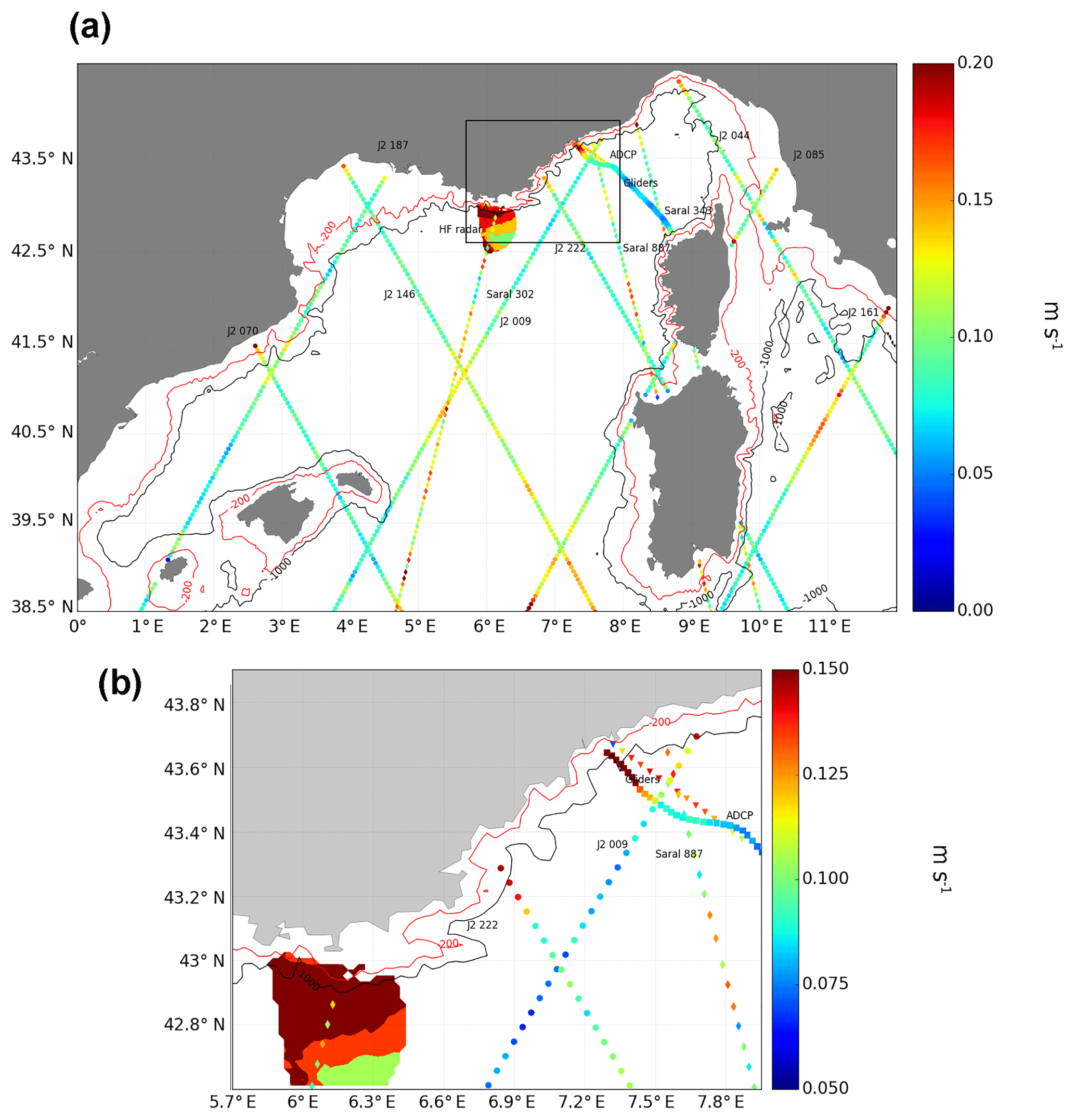
Figure 3(a) Map of the standard deviations of the velocities derived from ADCP, glider, HF radar and altimetry data over the period March 2013–October 2014. (b) Zoom-in view of the northern Ligurian Sea (black rectangle indicated in panel a); 200 m (red line) and 1000 m (black line) isobaths are also shown.

Download

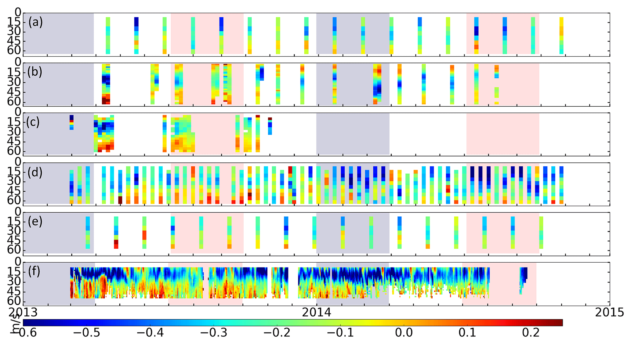
Figure 4Time–space diagrams of the current velocities derived from (a) SARAL track 887, (b) ADCP, (c) gliders, (d) Jason-2 track 222, (e) SARAL track 302, and (f) HF radars between March 2013 and October 2014. The pink and grey areas in the background of the diagrams correspond to the summer and winter seasons, respectively.

Download

Figure 3 represents the associated current variability, as captured by the different types of observations. Not surprisingly, in all datasets, larger standard deviation values generally coincide with the NC system. In altimetry, we observe values of 0.12–0.2 m s⁻¹ at the northern ends of the Jason-2 tracks 161, 085, 044, 222, 146 and 070 (the signal at the end of track 146 does not correspond to the NC) and SARAL tracks 302, 343 and 887. If we focus on Jason-2 track 222 in Fig. 3b, we first clearly see the coastal current variations associated with the NC flow (see also Fig. 2b). However, the NC is not fully resolved by 1 Hz altimetry data: observations stop at ∼10 km from land. The more coastal observations have been discarded during the processing, probably due to large data errors. This is even more true for the Jason-2 track 009 (the last data point available is associated with a large suspicious current value) and the SARAL tracks 887 and 302. We have to keep in mind that in this area, where the narrow NC flow is very close to the coastline (its core is in the range 10–40 km from land; Piterbarg et al., 2014), its observation by altimetry is very challenging. In comparison, the ADCP, glider and HF radar data allow us to observe the NC variability much closer to the coast: our datasets stop at 2.5, 3.5 and 3–7 km from land, respectively. But they all differ in the current variance captured. Concerning the ADCPs and gliders observing the NC at the same location, the ADCPs show larger standard deviation values (∼0.13 m s⁻¹) almost all along the transect, while the gliders show much lower values in the open ocean (∼0.05 m s⁻¹), increasing on the shelf break to values very close to the ones observed on Jason-2 track 222 (∼0.15–0.20 m s⁻¹). Further west, the HF radars show the largest current variance south of Toulon, with values around 0.23 m s⁻¹, located on the continental shelf break. In comparison, the corresponding NC variance captured by the SARAL track 302 is only half of that. Further south, off Corsica, the gliders show very low variability, roughly half of the values corresponding to the NC, indicating a WCC flow that is very stable in time (as also shown in Astraldi and Gasparini, 1992).

Considering the intrinsic and important differences between the different current datasets (Sect. 2.3), these first statistical results are encouraging. They give a coherent picture of the regional circulation, with, except for the HF radars that capture a faster current flow, about the same NC average velocity values. The NC variability is also clearly captured by the different datasets all along its path, but with significant differences in terms of amplitude. Note that when we recompute the standard deviations using a larger period of time (not shown), ADCPs and gliders tend to converge toward the same cross-shore profile as the one derived from Jason-2 track 222, with a maximum about 0.03 m s⁻¹ larger for the in situ observations. We can then conclude that this diagnostic is largely influenced by the number of data samples considered as well as by the period of time covered by the measurements.

In order to better understand the differences in variability captured by the various datasets, we analyze the time–space diagrams of the currents derived from ADCP, HF radar, glider and altimetry data over the period considered (Fig. 4). We focus on the first 60 km off the French coast and, concerning altimetry, on SARAL tracks 302 and 887 and on Jason-2 track 222. The HF radar data correspond to a meridional section of the zonal current component located at 6.2^∘ E. The NC is clearly detected in all data but Fig. 4 displays large variations at different timescales (see also Font et al., 1995; Sammari et al., 1995; Albérola et al., 1995) that make the data temporal sampling resolution a very sensitive question if we want to study this current system. The number of glider transects is low and concentrated in 2013, and the unevenly spaced ADCP sections miss a large number of events. Spring 2013 and winter and summer 2014 are poorly sampled. The HF radar provides a very good temporal sampling according to what is needed to capture the high-frequency NC variations, but it monitors only its section located in the vicinity of Toulon. Altimetry provides good complementary information. Despite its relatively low spatial resolution and the intrinsic difficulties when approaching the land, it detects seasonal changes coherent with the ones observed in the other datasets as well as much shorter period changes. Note that if the SARAL mission capabilities are expected to be particularly adapted for fine-scale oceanography and coastal applications (Verron et al., 2018), in our case study its 35-day period appears to be a strong limitation on monitoring the highly fluctuating NC flow. This particular point will be further analyzed in Sect. 3.3. In the next section, we concentrate on the seasonal variability observed in the different datasets, as it is known to be the dominant signal of the NC system at regional scale (Alberola et al., 1995; Sammari et al., 1995; Crépon et al., 1982; Birol et al., 2010).

3.2 The seasonal variability of the NC flow captured by the different instruments

Here we compare the monthly climatology (i.e., the mean value for each month of the year) of the maximum NC amplitude computed from the different current datasets (ADCP, glider, HF radar and altimetry). This time, we use all the data available during the period 1 January 2010–31 December 2016 (note that the HF radar data are only available over the period 2012–2014). Concerning altimetry, we consider only Jason-2 since we have two to four samples per month for SARAL, which is not enough to compute meaningful statistics (see Table 2). For each data sample available, the current profiles along the Jason-2 track 222, the ADCP and glider reference transects, and a meridional HF radar section located at 6.2^∘ E are analyzed. The maximum NC amplitude is defined as the average of the first decile of the velocity values for each transect and time (remember that the NC corresponds to negative current values). These values must be close in space. This strategy allows us to filter large isolated current values, which may not correspond to the NC. In altimetry, only a distance spanning 60 km to the coast is considered. The number of data points in the first decile varies according to the dataset and to the number of data in the section considered. Because of the lower resolution, it always corresponds to one point in altimetry. As we can see in Fig. 4d, data gaps exist in Jason-2 for some cycles. When more than three points are missing, the corresponding cycle is discarded from the analysis. Finally, all the maximum NC values collected are averaged as a function of month and dataset, and they are synthesized in monthly climatologies. The results derived from in situ data are in Fig. 5a and the results derived from altimetry are in Fig. 5b. The glider results are in both figures because this instrument provides the currents closest to altimetry in terms of physical content. For each month, the standard deviation computed from all the NC amplitude values available is also indicated.

Table 2 lists the temporal distribution of the number of samples included in the calculation as a function of month (in brackets). The data density is much more important than in Sect. 3.1 and the corresponding statistics more robust. It appears relatively stable for Jason-2 altimetry and more heterogeneous for the other observations. The number of in situ data points per month is strongly variable, especially for the ADCP and to a lesser extent for the glider, and varies also a lot from one year to another. A total of 24 ADCP transects are available in 2015 and only 7 in 2012 and 2014, while the glider dataset has a large gap in 2014. As a consequence, the results will only be discussed in terms of seasonal tendencies.

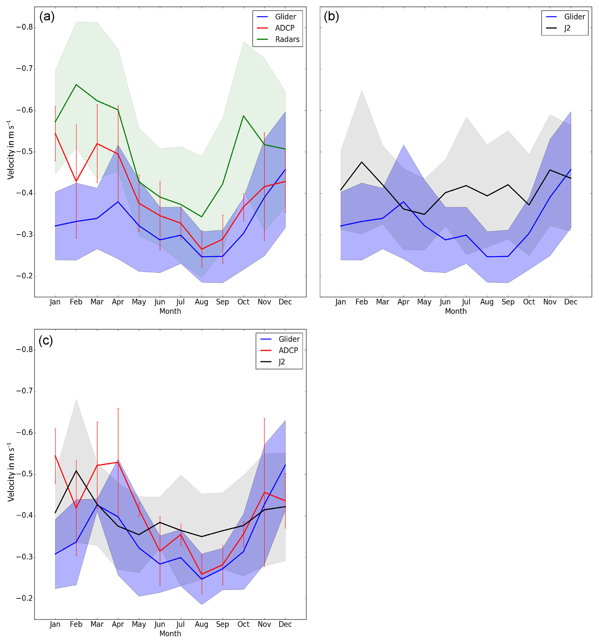
Figure 5Seasonal variations of the maximum current amplitude derived from the (a) HF radars (green line), ADCP (red line), gliders (blue line), and (b) Jason-2 (black line) and glider (blue line) observations available over the period 1 January 2010–31 December 2016. (c) Same as (a) and (b) but computed over the period July 2008 to June 2014 and only for the gliders, ADCP and Jason-2. For all the curves the monthly standard deviation of the maximum current amplitude derived from the corresponding instrument is also indicated (curve envelopes and error bars).

Download

In Fig. 5a and b, except altimetry, all the climatologies show a clear and coherent seasonal cycle of the NC amplitude, with a stronger–lower flow in winter–summer. As already seen in the previous section, compared to the other datasets, the HF radars capture a faster NC south of Toulon. Higher NC velocities are expected in this location (Ourmières et al., 2011). The corresponding amplitude of the seasonal variations is 0.32 m s⁻¹, with a minimum of −0.34 m s⁻¹ in August and a maximum of −0.66 m s⁻¹ in February. These values are also found by Guihou et al. (2013) in the same area. In comparison, further east in the northern Ligurian Sea, the peak-to-peak amplitude of the seasonal cycle is slightly lower for the ADCPs than for the HF radars and is associated with a lower mean flow, with a minimum of $\sim -\mathrm{0.27}$ m s⁻¹ in August and a maximum of −0.54 m s⁻¹ in January. Note, however, that the value observed in January may be less robust (or at least poorly representative of a mean monthly situation) since it is computed only with three data samples. Concerning the gliders, the peak-to-peak amplitude variation is ∼25 % lower than for the ADCPs, with a minimum of $\sim -\mathrm{0.25}$ m s⁻¹ in August–September and a maximum of −0.46 m s⁻¹ in December. Since these instruments measure velocities at very close locations, the differences may be mainly due to ageostrophic currents. The Jason-2 climatology displays significantly different results with a series of maxima ($\sim -\mathrm{0.46}$ m s⁻¹ in February and November) and minima ($\sim -\mathrm{0.35}$ m s⁻¹ in May and October).

Table 3List of the cases of relative co-localization in time between the glider, ADCP and altimetry current data, with the corresponding dates of observations.

Download Print Version | Download XLSX

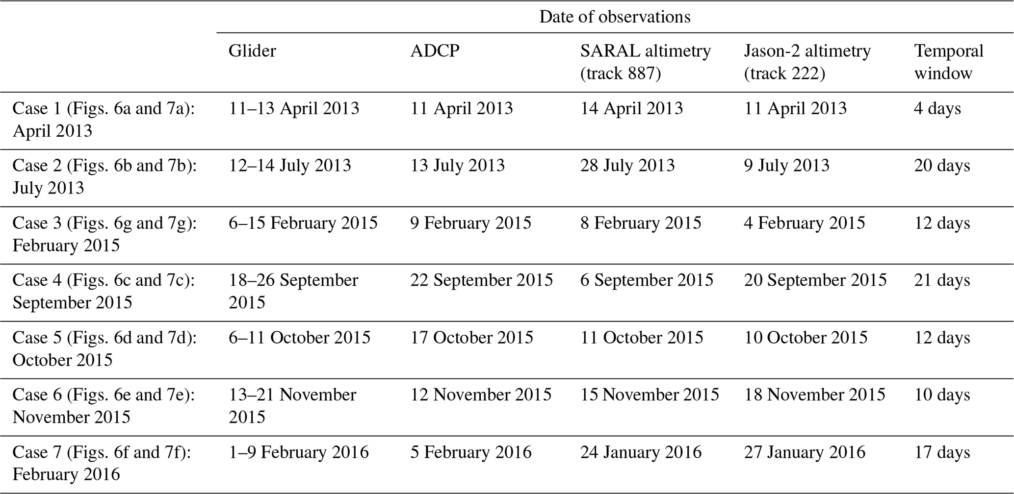
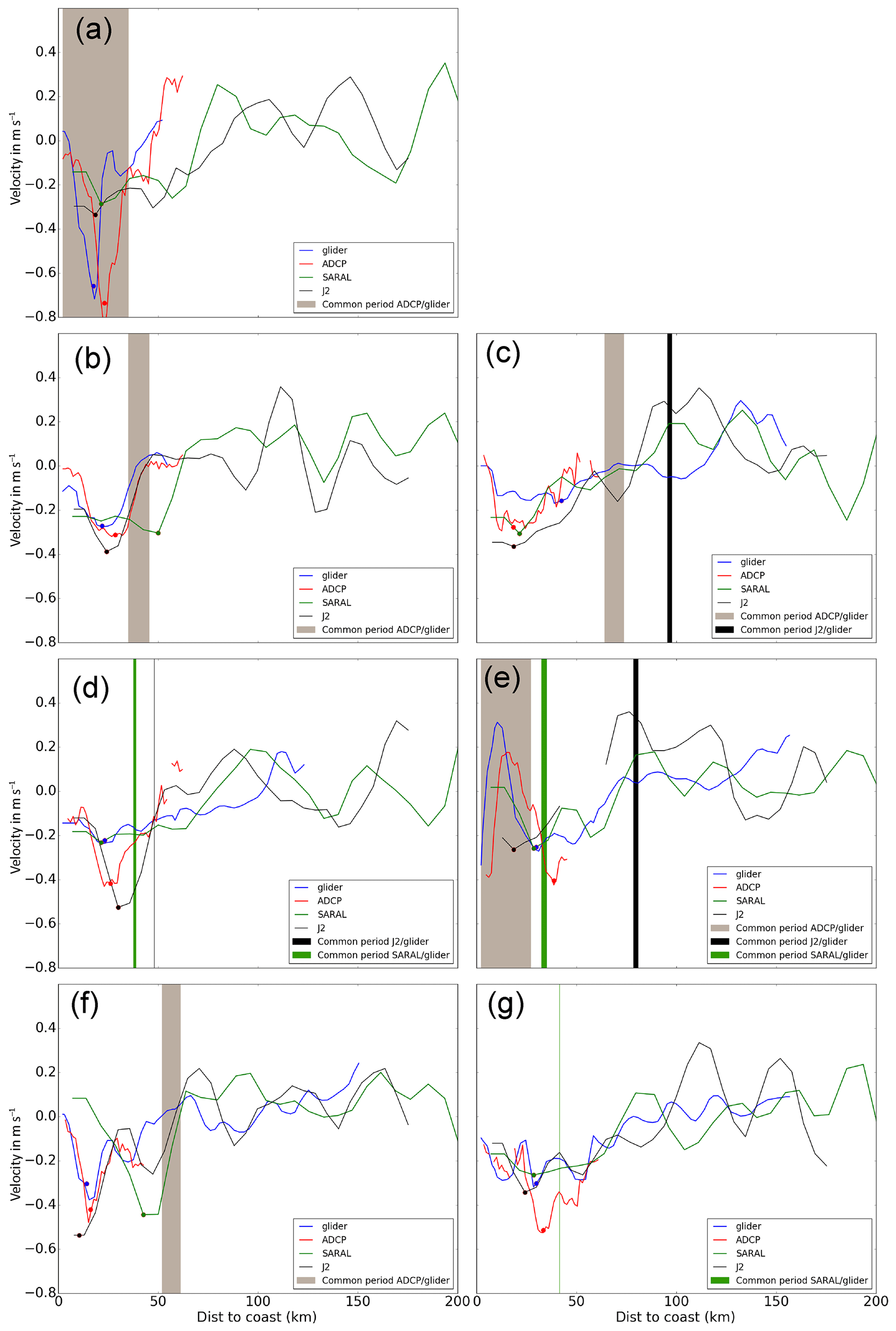
Figure 6Cross-shore sections of currents deduced from the glider (blue), ADCP (red), SARAL (green) and J2 (black) altimetry data for the seven individual cases identified in Table 3. Overlapping periods between the different observations are also indicated.

Download

For further analysis, we consider the dispersion of individual current values for each month (Fig. 5a, b, envelopes around the curves). We observe significantly different date-to-date variability for each month: between 0.03 and 0.15 m s⁻¹ for the glider and ADCP, between 0.12 and 0.20 m s⁻¹ for the HF radar, and between 0.08 and 0.17 m s⁻¹ for altimetry. It indicates that the seasonal NC cycle observed in Fig. 5 is modulated by a strong mesoscale and/or year-to-year variability, and it seems to be especially true during intermediate seasons. The dispersion curve of Jason-2 generally follows the other ones except in July and September, when it shows large peaks of variability. Deeper inspection of the corresponding current dataset reveals that it is due to much larger NC amplitudes observed during these months in 2014 and 2015. The corresponding NC intensifications are clearly observed in Fig. 4d in July and September 2014. Unfortunately, no glider transect is available during these periods (Fig. 4c) and we have only one ADCP section, which does not show an NC flow increase (Fig. 4b). However, the HF radar currents (Fig. 4f) tend to support the fact that the NC intensification captured by Jason-2 is realistic and not due to altimetry errors. One profile of SARAL track 887 is available in July 2014 and it exhibits the same feature (Fig. 4a). Since we did not find evidence of summer NC intensification in previous years, we decided to recompute the seasonal cycle of the NC amplitude using only the data available during the first 6-year period of Jason-2 (i.e., 2008–2014). We did the same for the ADCPs and gliders, but very few glider data and no ADCP currents are available before 2010. HF radar currents have not been considered because of the too-short length of the time series. The resulting curves are shown in Figure 5c and a clear seasonal cycle is now also observed in the climatology derived from Jason-2, with a summer–winter decrease–increase in the NC flow. Note that it is also coherent with the results of Birol et al. (2010), who used a combination of the T/P and Jason-1 altimeter missions to obtain a current time series over the 1993–2007 time period. The amplitudes of the seasonal variations computed during this new period of time are now around 0.29, 0.27 and 0.16 m s⁻¹ for the ADCP, glider and Jason-2 altimetry data, respectively. Figure 5c highlights the fact that the summer velocities measured by in situ instruments are relatively close on average. During winter and especially spring, the differences become significant in both amplitude and phase.

Two physical processes can explain the fact that the differences between the different types of current measurements vary as a function of season. First, the stronger mesoscale variability associated with the NC during winter and spring makes the space and time sampling of the current measurements a more critical issue for the study of this current system at that particular time of year. Second, the strong Tramontane and Mistral winds are more frequent in winter and spring. Then, the differences between the glider and the ADCP current measurements, very close in location, may be more important when the non-geostrophic dynamics (in particular the Ekman flow) produced by the strong winds are more important. The closest seasonal variations to the ones observed by altimetry are found for the glider. It is not surprising since the currents derived from this instrument are also the closest in terms of physical content (see Sect. 2.3). Despite the spatial resolution of the altimetry data and the width and very coastal location of the NC, the amplitude of its seasonal variations captured by the Jason-2 track 222 along the French coast is 55 %–60 % of the amplitude captured by both the gliders and ADCPs.

3.3 Individual snapshots

To learn more about the similarities and differences between the currents derived from the different instruments, as well as their causes, we now analyze the observations on particular dates. In order to minimize, as far as possible, the differences due to distances in space and time between observations, we focus here on the region near Nice (i.e., on the ADCP and glider data, as well as on SARAL track 887 and Jason-2 track 222) and consider only observations that are close in time. For each day of the 2010–2016 study period, we used a time window for each dataset: 5 days for Jason-2, 10 days for the glider and ADCP data, and 22 days for SARAL. We selected only the dates for which the four types of observations are available and finally obtained seven cases that are reported in Table 3. The corresponding cross-track currents are shown in Fig. 6 (by season) as a function of the distance to the point at which the corresponding transect intersects the coastline. For each case and each dataset, we have computed the maximum NC amplitude, following the same method as in Sect. 3.2, and the corresponding location. The latter is expressed in terms of distance to the coast. The results are provided in Table 4.

Figure 6 highlights very different NC situations. Here, the largest coastal current velocities are observed in spring and not in winter as expected from Sect. 3.2. Case 1 (Fig. 6a), the only one in this season, shows by far the strongest NC amplitudes in ADCP and glider data ($<-\mathrm{0.6}$ m s⁻¹) associated with a narrow flow located within the 30 km coastal band. It corresponds to a difficult study case for altimetry, which is still able to depict the NC, but with a too-large current vein with an amplitude less than half of what is observed in the in situ observations. Cases 2 and 4 (Fig. 6b, c) are in summer. The NC is broader and its velocity is around −0.3 m s⁻¹ in all datasets, except in the glider of case 4 (see below). This time, altimetry successfully captures the NC amplitude; the location of its core is also good in case 4 but not in case 2 (it is too far to the coast for SARAL). In case 4, altimetry and ADCP currents are very close but, for a reason that is unclear (it may be due to an NC meander or eddy captured by the glider and not by the other instruments), the glider represents a significant slower flow located further south. Cases 5 and 6 (Fig. 6d, e) both correspond to autumn situations but they highlight very different coastal current patterns. In case 5, the glider and SARAL data corresponding to the same day are very coherent: they show a relatively weak NC flow ($\sim -\mathrm{0.2}$ m s⁻¹) with a core ∼30 km to the coast. Jason-2 observations, very close in time to SARAL and the glider data, show a larger current located slightly further south (∼6 km). The ADCP represents an NC vein at the same location as the glider and SARAL but with a much stronger amplitude. It could be due to the differences in the dates of observations (1 week from Table 3, the temporal scale at which meanders develop) or an important ageostrophic NC component. In case 6, a lack of data for Jason-2 can be observed, which leads us to question the realism of the current estimates close to the coast. However, the glider, the ADCP and SARAL data show a broad NC located further offshore than in the other cases. Its core is located ∼40 km offshore in ADCP and glider data. As in case 5, the glider and SARAL data provide NC amplitudes and locations that are relatively close and the ADCP data give a larger NC maximum. A particular feature in this autumn situation is the succession of very strong and narrow southwestward and then northeastward flows observed in the first 20 km of the coastal band in both ADCP and glider currents. It is not captured by SARAL, which does not get close enough to the coast. It is probably associated with an eddy or meander stuck on the northern anticyclonic side of the NC (eddies were documented at this location in Casella et al., 2011). Finally, cases 3 and 7 (Fig. 6g, f) correspond to winter situations and, as for the autumn, they are very different. In case 3, we observe a broad NC with a core located around 30 km to the coast. The glider exhibits current oscillations along its transect but all current datasets show a coherent representation of the NC, even if the ADCP data provide larger velocities. In case 7, the glider and ADCP capture a narrow NC located ∼20 km off the coast also observed by altimetry but with some differences: in Jason-2 the NC flow is not entirely captured and in SARAL it is located further offshore. It may be due to rapid variations in the NC between the different dates of observations: 12 days between ADCP and SARAL.

Beyond the large variations in the NC characteristics from one case to another, an interesting feature in Fig. 6 is the presence of an eastward flow located south of the NC (i.e., 100–150 km to the coast) in altimetry data in different cases (cases 4, 5 and 6 in particular). The ADCP transect is too short to capture this current vein and it is not observed in the glider data, located further east compared to SARAL track 887 and Jason-2 track 222. The latter rather depict the WCC on the southern edge of its section. To our knowledge, this offshore eastward flow is not documented in the literature but its signature also seems to be observed in Figs. 2a and 3a (around 42.5^∘ N in SARAL and around 42.8^∘ N in Jason-2). It will be further discussed in Sect. 3.5.

Finally, what is illustrated in Fig. 6 is that, because of the large short-term changes in the NC circulation system, each snapshot of observations differs significantly from the corresponding seasonal average. It highlights the strong interest in long-term and regular altimetry data to study the persistent components of the NC circulation system, as well as its seasonal variations and possible longer-term changes.

Figure 7Same as Fig. 6 but for HF altimetry data.

Download

3.4 Can we improve the estimation of the NC characteristics with high-rate altimetry compared to 1 Hz data?

In this section we consider the improvement that is possible to obtain in terms of current derivation with the use of high-rate altimetry measurements, compared to the conventional 1 Hz data used above. However, if research coastal altimetry products that are calibrated, validated, and cover different regions and missions are now available at 1 Hz, this is not the case for high-rate altimetry products. Even if some studies have shown the better performance of 20 and 40 Hz altimeter measurements in observing coastal circulation (Birol and Delebecque, 2014; Gomez-Enri et al., 2016), they are much noisier and there is no consensus yet concerning their (post-)processing. Here, we used an experimental version of high-rate X-TRACK SLA data for both Jason-2 and SARAL, for which original measurements are at 20 and 40 Hz, respectively. Since a lot of erroneous data remained in the coastal area, we applied a 2-sigma filter on the resulting SLA fields along each individual track and cycle in order to edit the data before filtering and the computation of the current estimates (Sect. 2.1).

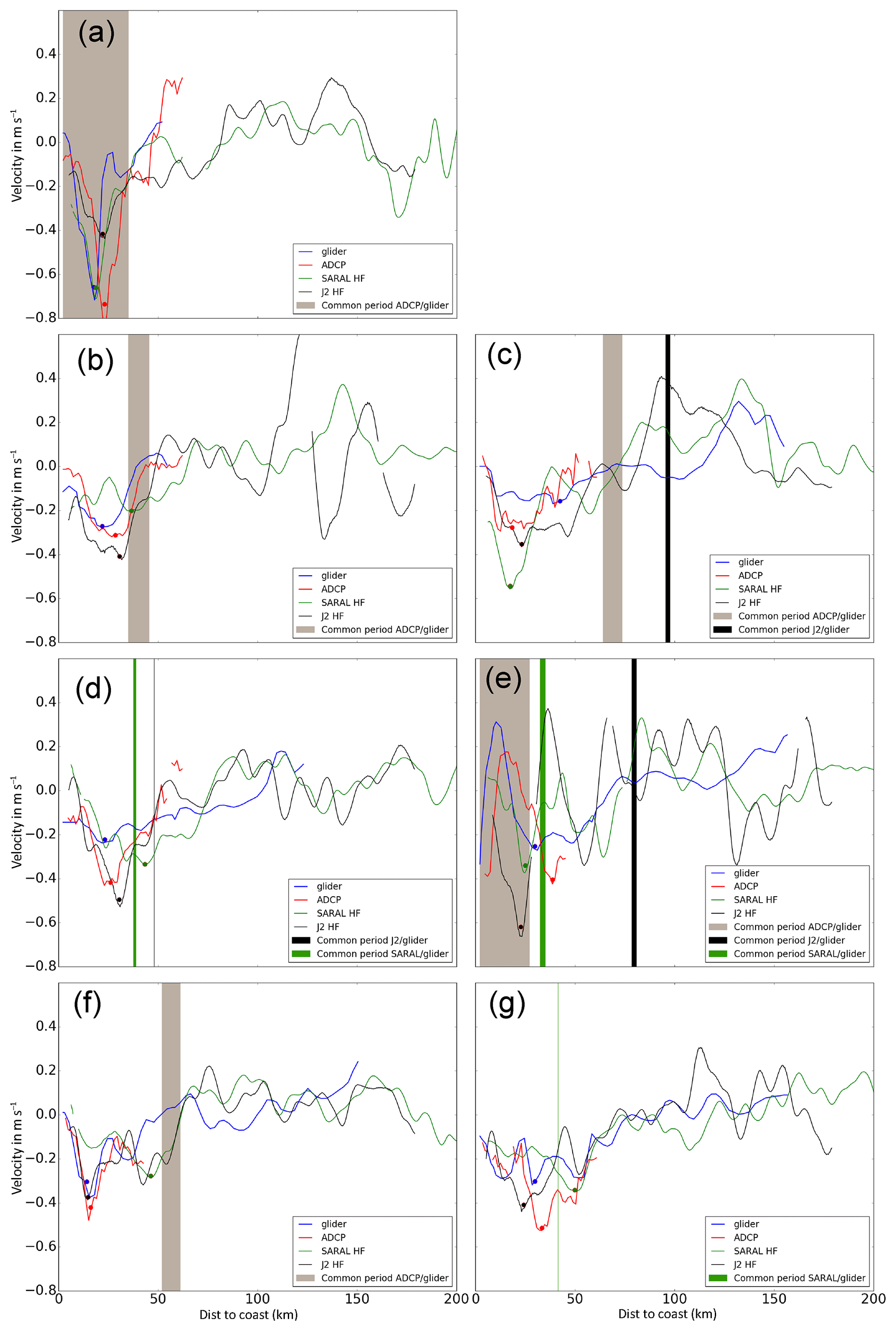
In order to analyze if we can expect a better observation and understanding of NC variations from high-rate altimetry measurements, they have been used to compute the same diagnostics as in Sect. 3.1, 3.2 and 3.3. Only the results for the individual snapshots will be illustrated here (Fig. 7) since, even if the major difference with the current fields derived from 1 Hz altimetry is that the larger number of coastal data points allows us to estimate currents closer to the coast and then to better resolve the NC flow (see Fig. 7), we did not find significant differences in the NC statistics (i.e., mean current and standard deviation values) or the amplitude of the seasonal cycle computed from 20 and 40 Hz SLA compared to the 1 Hz solutions.

Table 4Maximum NC value and distance to the coast of this maximum deduced from the glider, ADCP and altimetry current data for the seven individual cases listed in Table 3.

Download Print Version | Download XLSX

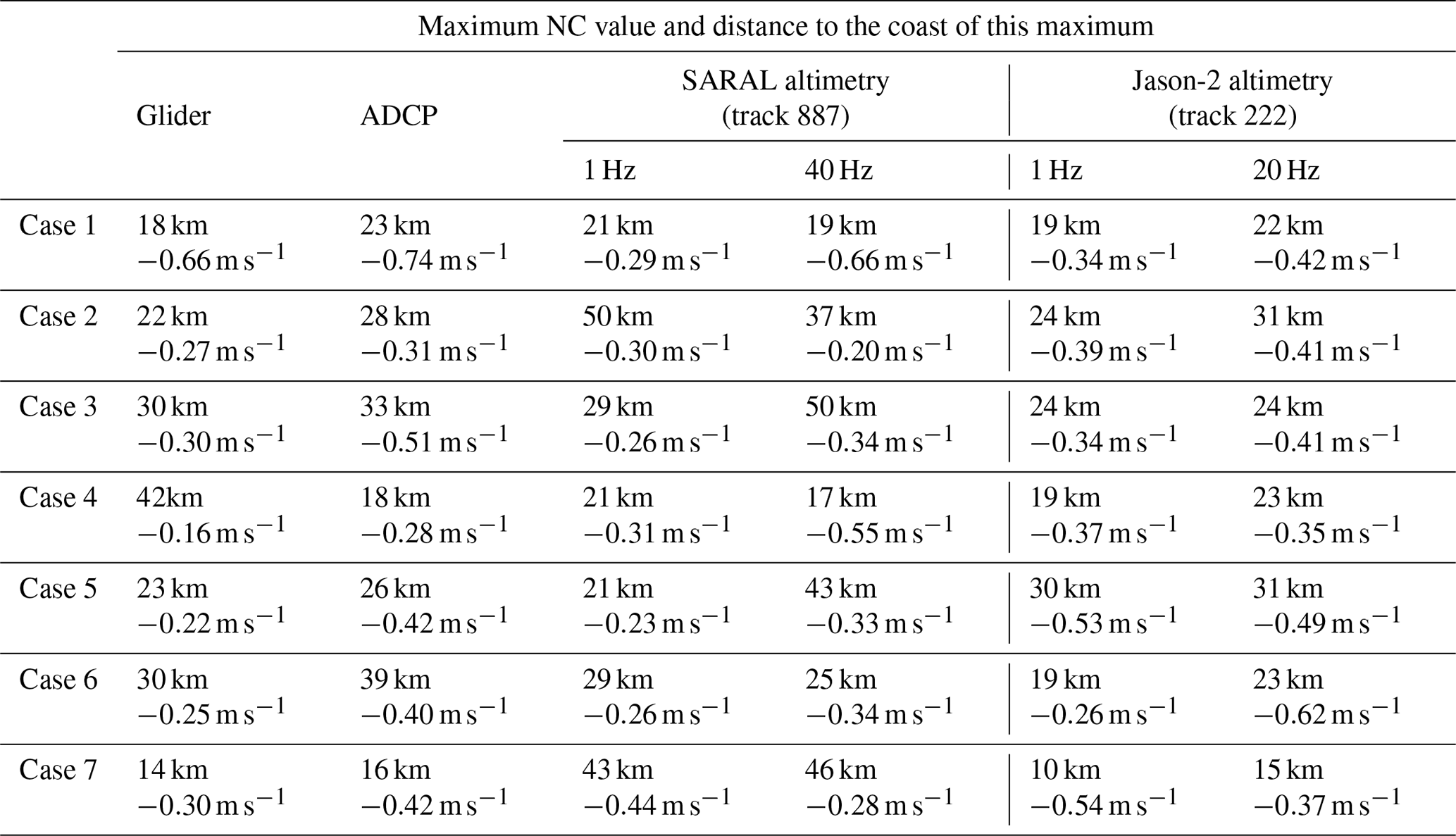
In Fig. 7, the same color code as in Fig. 6 is used. For each case, as in Sect. 3.3, the maximum NC amplitude and corresponding location are reported in Table 4 for both SARAL and Jason-2. In case 1 (Fig. 7a), the gain obtained with the use of HF data is very clear. On this date the NC vein is narrow and located near the coast. Contrary to the 1 Hz solution, the NC is better resolved by both SARAL and Jason-2 high-rate altimetry. It is especially true for SARAL with NC characteristics that are almost identical to the ones derived from the gliders. In Jason-2, the NC core is also close to the glider solution but its amplitude is ∼35 % lower. For cases 2 and 4, which correspond to the summer (Fig. 7b and c), here again the use of high-rate altimetry allows for the better observation of an NC vein but the agreement with in situ data is not so good. Concerning SARAL, for case 2, the current estimates are suspect since a reduction of the current intensity appears at the location of the NC core in the other datasets (Fig. 7b). For case 4, SARAL NC amplitude is too high: 0.55 m s⁻¹ vs. 0.16 m s⁻¹ for the glider. Jason-2 high-rate NC estimates appear closer to the in situ data than SARAL for both cases 2 and 4, but the resulting NC characteristics do not appear better than the corresponding 1 Hz estimations when compared to ADCP (Table 4). It probably reveals that the cutoff frequency chosen in the filtering is too low. Cases 5 and 6 (Fig. 7d and e) also show some very doubtful oscillations in both SARAL and Jason-2 currents, and high-rate altimetry does not improve the NC estimations. In winter, the cases 3 and 7 (Fig. 7g and f, respectively) are very different. In case 7, 20 Hz Jason-2 data depict the entire NC with current estimates much closer to in situ data (especially the glider) compared to 1 Hz Jason-2 measurements. In case 7 they degrade–improve the NC representation (Fig. 7g) if we refer to the glider–ADCP, respectively. Note that this case illustrates the difficulty of the calibration of altimetry data processing algorithms with independent observations since results may differ as a function of the independent observations used. Here, 40 Hz SARAL data show a too-noisy current solution.

As already shown in previous work (Birol and Delebecque, 2014; Gomez-Enri et al., 2016), high-rate altimetry allows us to derive significantly more sea level data near the coast. Here we observe that the coastal circulation derived is better resolved in space, both in terms of horizontal resolution and distance to the coast of the current estimates. However, the resulting current fields depend crucially on the strategy followed for data processing, including retracking, corrections, screening and filtering.

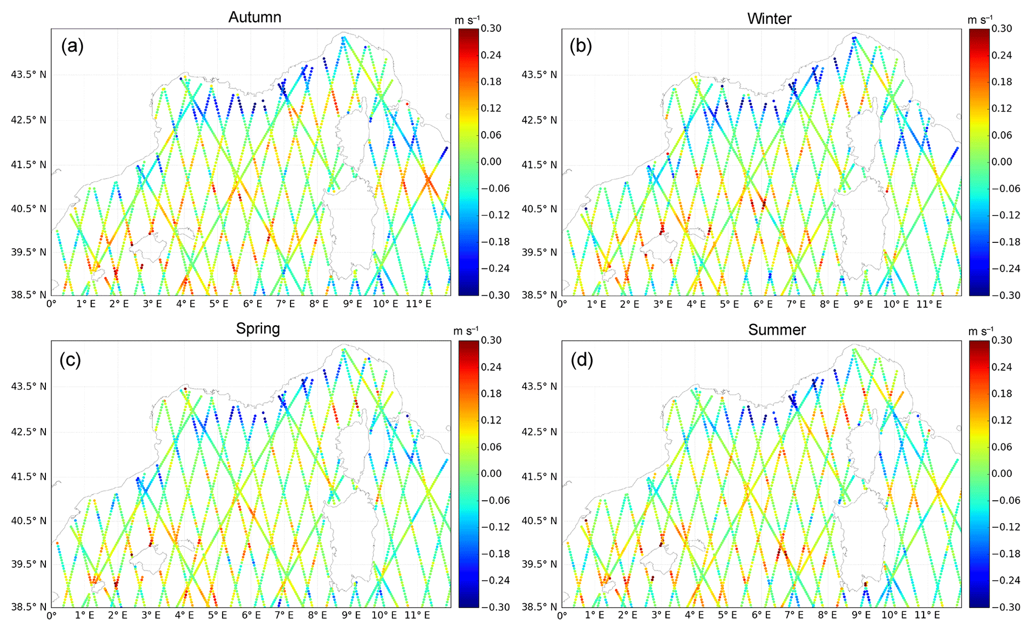
Figure 8Seasonal climatology maps of cross-track geostrophic currents (in m s⁻¹) derived from Jason-2 and SARAL/AltiKa altimeter data over the period April 2013–April 2016.

Download

3.5 The seasonal variability of the regional surface circulation observed by altimetry

Here we use only 1 Hz altimetry data. In order to separate the seasonal component of the surface circulation from the mesoscale variations, along each pass of Jason-2 and SARAL located in the area of interest, we have computed a seasonal “climatology” of the cross-track surface geostrophic currents captured by these two altimetry missions (Fig. 8). It was done by simply averaging the corresponding seasonal velocity values for the common 3-year period: April 2013–April 2016. Note that this type of analysis can also be found in Birol et al. (2010) with a much longer period of altimetry data, but with Jason measurements only. The need to use multi-mission observations was incidentally pointed out in this study. Here, indeed, the combination with SARAL data largely improves the spatial resolution of the regional circulation, enabling us to capture the main current veins at many more locations along their path (see Fig. 9 of Birol et al., 2010, for comparison).

In Fig. 8, all the structures of the standard circulation scheme in the NW Mediterranean Sea (Fig. 1) are observed: the NC, the WCC, the Balearic Current, the Balearic Front and the TC. What can also be noticed first is the very good coherence and complementarity between the SARAL and Jason-2 climatologies, especially at crossover points. The seasonal variations in the regional circulation system, already discussed in detail in Birol et al. (2010), are confirmed from this different and shorter period of altimetry observations. In particular, if a stronger and unique southwestward flow is observed along the Italian, French and Spanish coasts from autumn to spring, it is not so clear during summer. During this season, the NC does not seem to continue west of 4^∘ E to reach the Balearic Sea. Instead, it may recirculate eastward offshore of Cape Creus.

More generally, compared to Birol et al. (2010), the better spatial coverage obtained by combining both SARAL and Jason-2 reveals a circulation scheme that could be much more complex than the one classically proposed in the literature. In summer and autumn (Fig. 8a, d), between 3 and 9^∘ E, individual eastward current veins are observed between the NC and the Balearic Front, suggesting that recirculations may exist along its path during these seasons. One of them corresponds to the eastward current branch mentioned in Sect. 3.3. Note, however, that this seasonal analysis is based only on 3 years of observations and could be biased by particular features occurring during 2015. Further investigation based on numerical modeling is clearly needed. This is the next step of this study. Here again, altimetry clearly appears to be a very good tool to validate the model results.