Tidal resonance in the Gulf of Thailand

Cui, Xinmei; Fang, Guohong; Wu, Di

doi:https://doi.org/10.5194/os-15-321-2019

Articles | Volume 15, issue 2

https://doi.org/10.5194/os-15-321-2019

Articles | Volume 15, issue 2

Research article

29 Mar 2019

Research article |

| 29 Mar 2019

Tidal resonance in the Gulf of Thailand

Xinmei Cui, Guohong Fang, and Di Wu

Abstract

The Gulf of Thailand is dominated by diurnal tides, which might be taken to indicate that the resonant frequency of the gulf is close to one cycle per day. However, when applied to the gulf, the classic quarter-wavelength resonance theory fails to yield a diurnal resonant frequency. In this study, we first perform a series of numerical experiments showing that the gulf has a strong response near one cycle per day and that the resonance of the South China Sea main area has a critical impact on the resonance of the gulf. In contrast, the Gulf of Thailand has little influence on the resonance of the South China Sea main area. An idealized two-channel model that can reasonably explain the dynamics of the resonance affecting the Gulf of Thailand is then established in this study. We find that the resonant frequency around one cycle per day in the main area of the South China Sea can be explained with the quarter-wavelength resonance theory, and the large-amplitude response at this frequency in the Gulf of Thailand is basically a passive response of the gulf to the increased amplitude of the wave in the southern portion of the main area of the South China Sea.

Download & links

Article (PDF, 6822 KB)

How to cite

How to cite.

Dates

Received: 12 Aug 2018 – Discussion started: 24 Aug 2018 – Revised: 01 Feb 2019 – Accepted: 18 Feb 2019 – Published: 29 Mar 2019

1 Introduction

The Gulf of Thailand (GOT) is an arm of the South China Sea (SCS), the largest marginal sea of the western Pacific Ocean (Fig. 1). The width of the GOT is approximately 500 km, and the length of the GOT from the top to the mouth of the gulf, as indicated by the blue B line in Fig. 1, is approximately 660 km. The mean depth in this area is 36 m according to the ETOPO1 depth data set (from the US National Geophysical Center). The mean depth of the SCS from the southern opening of the Taiwan Strait to the cross section at 1.5^∘ N is 1323 m. If the GOT is excluded, the mean depth of the rest of the SCS (herein called the SCS body and abbreviated as SCSB) is 1457 m. Tidal waves propagate into the SCS from the Pacific Ocean through the Luzon Strait (LS) and mainly propagate in the southwest direction towards the Karimata Strait, with two branches that propagate northwestward and enter the Gulf of Tonkin and the GOT. The energy fluxes through the Mindoro and Balabac straits are negligible (Fang et al., 1999; Zu et al., 2008; Teng et al., 2013). The GOT is dominated by diurnal tides, and the strongest tidal constituent is K₁ (Aungsakul et al., 2011; Wu et al., 2015).

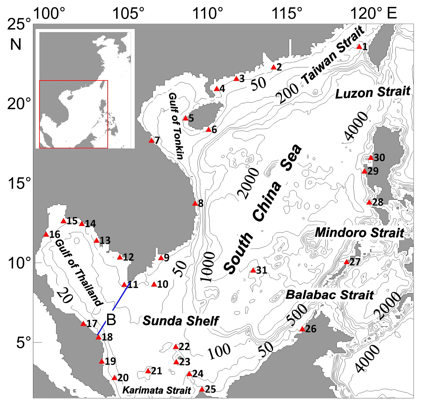
https://www.ocean-sci.net/15/321/2019/os-15-321-2019-f01

Figure 1The South China Sea and its neighboring area. The contours show the water depth distribution in meters. The blue B line is the mouth cross section of the Gulf of Thailand (GOT). The triangles represent the tidal gauge stations (the full names of these stations are given in Table 1). The inset in the upper-left corner shows the entire model domains (99–131^∘ E, 1.5–42^∘ N).

Download

The resonant responses of the GOT to tidal and storm forcing have attracted extensive research interest. However, the previous results have been diverse. Yanagi and Takao (1998) simplified the GOT and Sunda Shelf as an L-shaped basin and concluded that this basin has a resonant frequency near the semi-diurnal tidal frequency. Sirisup and Kitamoto (2012) applied a normal mode decomposition solver to the GOT and Sunda Shelf area and obtained four eigenmodes with modal frequencies of 0.42, 1.20, 1.54 and 1.76 cpd (cycles per day). Tomkratoke et al. (2015) further studied the characteristics of these modes and concluded that the mode with a frequency of 1.20 cpd is the most important. Cui et al. (2015) used a numerical method to estimate the resonant frequencies of the seas adjacent to China, including the SCS and the GOT, and found that the GOT has a major resonant frequency of 1.01 cpd and a minor peak response frequency of 0.42 cpd. In these studies, except for Yanagi and Takao (1998), no effort was made to establish a theoretical model of the GOT, and the resonant period estimated by Yanagi and Takao (1998) cannot be used to explain the resonance of the diurnal tides.

The GOT is a semi-enclosed gulf with an amphidromic point in the basin for each K₁ and O₁ constituent. Wu et al. (2013) reproduced the tidal system well with superimposed incident and reflected Kelvin waves and a series of Poincare modes. This result raises the question of whether the quarter-wavelength resonant theory can explain the tidal resonance in the gulf, as is the case with other areas (Miles and Munk, 1961; Garrett, 1972; Sutherland et al., 2005). According to quarter-wavelength theory, because the distance from the head of the gulf to the mouth is approximately 660 km and the mean depth is approximately 36 m, the resonant frequency should be 0.61 cpd, which is much lower than the estimates by Cui et al. (2015) and Tomkratoke et al. (2015). Thus, it is clear that the tidal resonance phenomenon in the GOT cannot be reasonably explained by the quarter-wavelength theory.

According to the theories of Garrett (1972) and Miles and Munk (1961), tidal oscillations are limited to a specific area. In contrast, Godin (1993) proposed that tides are a global phenomenon that cannot be separated into independent subdomains. The GOT is an auxiliary area of the SCS and is connected to the SCSB. We thus believe that Godin's theory is applicable to the GOT. In this paper, by considering the bathymetry of the SCSB in numerical experiments and theoretical analyses, we investigate the reasons for the GOT to have a strong response around the frequency of one cycle per day and how the physical properties of the SCSB primarily determine the resonances of both the SCSB and the GOT.

2 The numerical model

2.1 Governing equations and model configuration

In this paper, we use the Princeton Ocean Model (POM) for numerical investigation, but we partially modify its code to meet the needs of the present study. This study is limited to the main mechanism of diurnal tidal resonance; accordingly, the elimination of tide-generating forces and nonlinear terms and the linearization of bottom friction in the control equation will not affect the problem we are studying, and the two-dimensional model effectively suits our purpose, as shown in a number of previous studies (e.g., Garrett, 1972; Godin, 1993; Webb, 2014; Cui et al., 2015). The general forms of the equation of continuity and the equation of motion used in this study are as follows:

\begin{array}{l} (1) & \frac{\partial \tilde{ζ}}{\partial t} = - \frac{1}{R \cos φ} [\frac{\partial (H \tilde{u})}{\partial λ} + \frac{\partial (H \tilde{v} \cos φ)}{\partial φ}], \\ (2) & \frac{\partial \tilde{u}}{\partial t} = 2 Ω \tilde{v} \sin ϕ - \frac{g}{R \cos φ} \frac{\partial \tilde{ζ}}{\partial λ} - \frac{τ \tilde{u}}{H}, \\ (3) & \frac{\partial \tilde{v}}{\partial t} = - 2 Ω \tilde{u} \sin ϕ - \frac{g}{R} \frac{\partial \tilde{ζ}}{\partial φ} - \frac{τ \tilde{v}}{H}, \end{array}

where t denotes time; λ and ϕ, respectively, refer to the east longitude and north latitude; $\tilde{ζ}$ is the surface height above the undisturbed sea level; $\tilde{u}$ and $\tilde{v}$ represent the east and north components of the fluid velocity, respectively; R indicates the Earth's radius, Ω its angular velocity, g gravity, H the undisturbed water depth and τ the linearized bottom friction coefficient.

The numerical model covers the ocean lying between 99, 131^∘ E, 1.5 and 42^∘ N. The northern and eastern open boundaries are located far beyond the area of the SCS to prevent the numerical values at the open boundaries from influencing the results in the study area. The southern open boundary is set along a zonal section of 1.5^∘ N, which meets the southernmost tip of the Malay Peninsula. The grid resolution is 1∕12^∘. The water depths are basically taken from the ETOPO1 data set and are modified using depth data extracted from navigational charts.

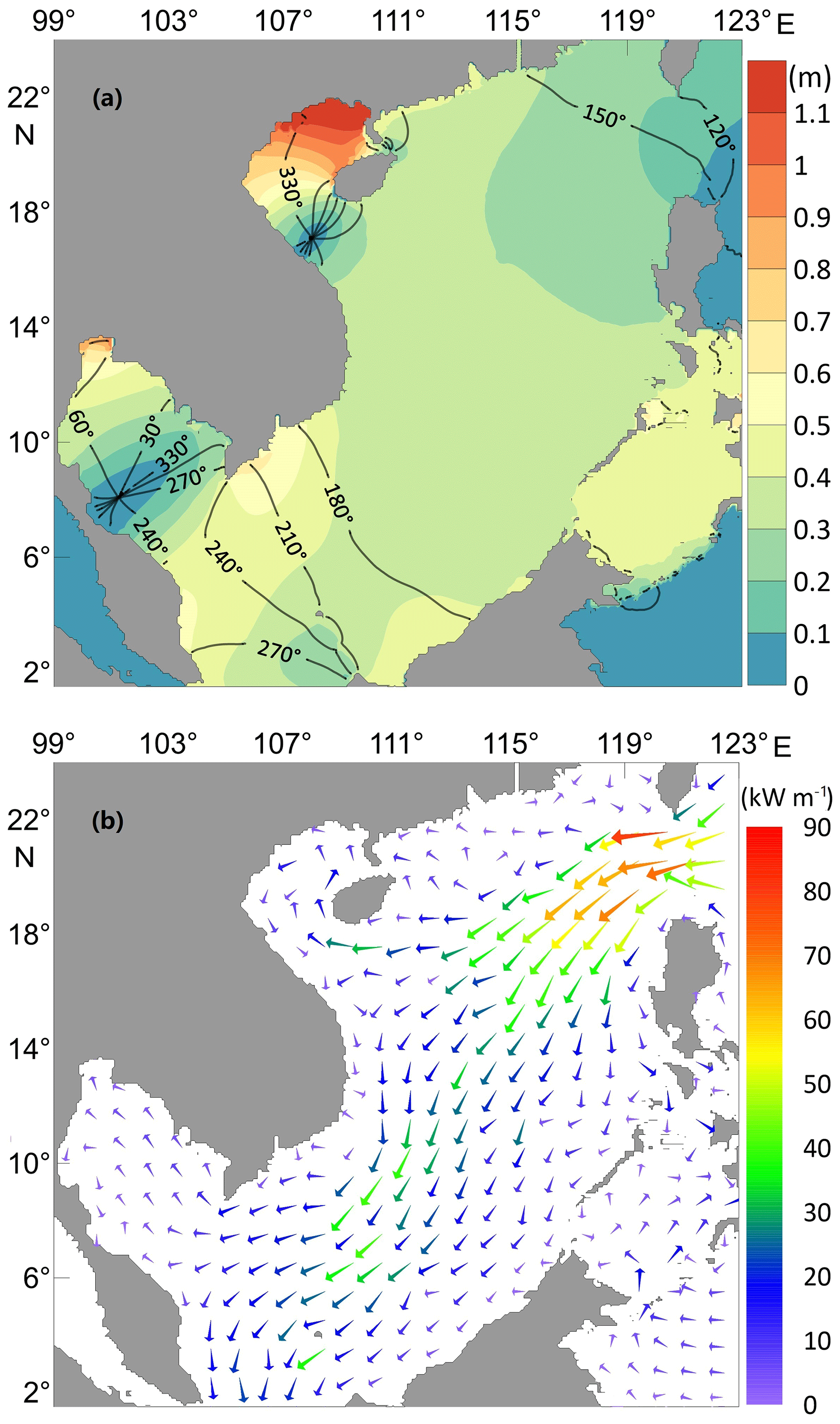
https://www.ocean-sci.net/15/321/2019/os-15-321-2019-f02

Figure 2Model-produced K₁ tidal system. (a) The distribution of Greenwich phase lags (in degrees) and amplitudes (color, in meters). (b) Tidal energy flux density vectors (in kW m⁻¹).

Download

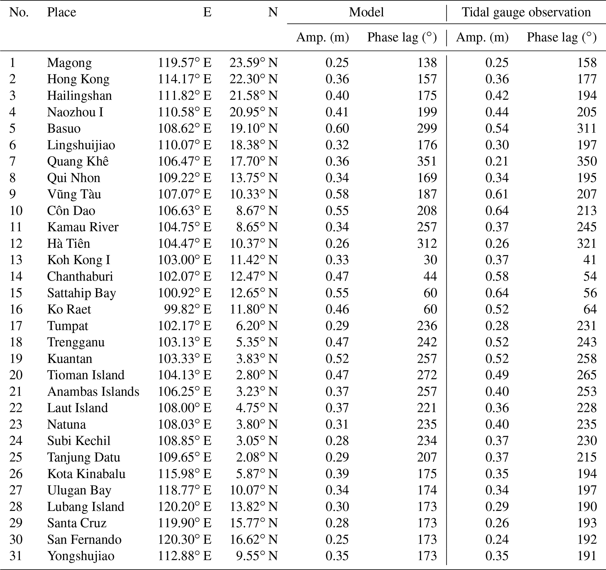
Table 1Comparison between model-produced and observed K₁ tidal amplitudes (m) and phase lags (degrees refer to Greenwich time).

Download Print Version | Download XLSX

2.2 Simulation of the K₁ tide

To examine the applicability of the modified POM model to the study area, the model is first used to simulate the K₁ tide in the SCS and its neighboring area. The amplitudes and phase lags along the open boundary are taken from the global tidal model TPXO9, which is based on satellite altimeter observations (Egbert and Erofeeva, 2002). The model-produced K₁ tidal system is shown in Fig. 2a, and a comparison of the model results with observations at 31 tidal gauge stations is shown in Table 1. The locations of these tidal stations are shown in Fig. 1, from which it can be seen that the stations are basically evenly distributed along the coast of the SCSB and GOT.

From Table 1, we can see that the deviations in amplitudes are mostly within 0.05 m, while those in phase lags are mostly within 20^∘. Considering that the governing equations are greatly simplified, the linearized bottom friction is used to replace the more accurate quadratic form, the agreement between model results and observations can be regarded as satisfactory. Therefore, the modified model is applicable to the SCS and GOT tidal study.

To show the characteristics of the wave propagation process, we calculate the tidal energy flux density distribution, as given in Fig. 2b. One can see that the K₁ tidal wave mainly enters the SCS through the LS and spreads southward, partially moves to the GOT and partially exits the SCS through the Karimata Strait. Figure 2a shows that the K₁ tidal amplitudes are large in the Gulf of Tonkin and that there is an amphidromic point at the mouth of the gulf caused by one-quarter-wavelength resonance (Fang et al., 1999). In the GOT, there is also an amphidromic point, but away from the mouth section, indicating that the amplified K₁ tide cannot be attributed to the quarter-wavelength resonance.

3 Numerical methods for estimating the resonant frequency

3.1 Open boundary condition

The open boundary condition for the tidal resonant study can be written in the following form:

\begin{matrix} (4) & \tilde{ζ} (i, j, t) = \sum_{n = N_{i}}^{N_{2}} {\tilde{Z}}_{n} (i, j) \cos [2 π f_{n} t - {\tilde{θ}}_{n} (i, j)], \end{matrix}

where (i,j) indicates grid points on the open boundary; f_n=nΔf refers to the frequency of the nth wave of interest, with Δf referring to the spectrum resolution; and for $n = N_{1}, N_{1} + 1, \dots, N_{2}$ , ${\tilde{Z}}_{n}$ and ${\tilde{θ}}_{n}$ represent the amplitude and phase lag of the nth wave, respectively. In this study, we choose $Δ f = 1 / 1024$ cph (cycles per hour) for the following two reasons. First, the value 1024 is equal to 2¹⁰, enabling us to efficiently calculate spectra from model-produced time series by using a fast Fourier transform (FFT). Second, because the minimum frequency difference between the main tidal constituents (Q₁, O₁, K₁, N₂, M₂ and S₂) is equal to $1.51 \times 10^{- 3}$ cph, the resolution of $Δ f = 1 / 1024$ cph is sufficient for separating these constituents.

3.2 Numerical model of the seas adjacent to China

Through the simulation of the K₁ tide, it is shown that the modified model can be applied to tidal study. The model setting is consistent with the setting of the simulation of the K₁ tide except that the water level values at the open boundaries are changed as follows. The amplitudes ${\tilde{Z}}_{n}$ at the open boundaries are specified as a constant, 2 cm; the phase lags ${\tilde{θ}}_{n}$ are given as random numbers that are evenly distributed in the interval (0,2π) and generated using a normal random number generator. The purpose of using random phase lags is to avoid all or some of the waves to have the same phase at a certain time, which can lead to simultaneous unreasonably high or low sea levels. The selected N₁ and N₂ values are 1 and 107, respectively. Thus, the frequencies of the waves studied range from 1∕1024 to 107∕1024 cph or 0.0234–2.5078 cpd. The corresponding periods range from 10 to 1024 h (approximately 0.4–42.7 days), which covers all main tidal constituents.

The model is run for 3×1024 h (see Cui et al., 2015, Fig. 2). In the last cycle of 1024 h, the hourly results at each grid point are preserved, and FFT analysis is performed to yield amplitude Z_n and phase lag θ_n. The amplitude ratio is defined as follows:

\begin{matrix} (5) & G_{n} = Z_{n} / {\tilde{Z}}_{n}, \end{matrix}

and the phase lag difference is given by the following equation:

\begin{matrix} (6) & ψ_{n} = θ_{n} - {\tilde{θ}}_{n} . \end{matrix}

According to Munk and Cartwright (1966), Ge^−iψ is the admittance. Specifically, as Munk and Cartwright (1966) stated, G_n is the amplitude response and represents the amplification factor of the nth wave in response to forcing. In the present study, we call G_n and ψ_n the amplitude gain and phase change, respectively, in accordance with Sutherland et al. (2005) and Roos et al. (2011).

4 Influence of resonance in the main area of the South China Sea on the Gulf of Thailand

Cui et al. (2015) revealed that both the SCS and GOT have strong response peaks around one cycle per day and suggested that the resonance of the SCS could be explained by one-quarter-wavelength resonance theory, but the authors did not provide the reasons for the strong response of the GOT around this frequency. As an arm of the SCS, the tidal energy of the GOT comes mainly from the SCSB (Fig. 2b), so we speculate that the strong response of the GOT around one cycle per day may be related to the SCS resonance.

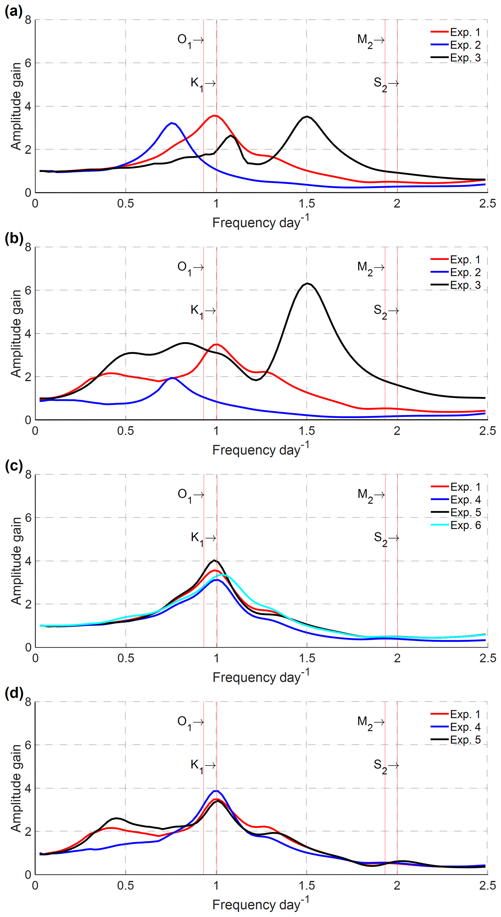
https://www.ocean-sci.net/15/321/2019/os-15-321-2019-f03

Figure 3Response functions (amplitude gains as a function of frequency) of the South China Sea body (SCSB) (a) and the Gulf of Thailand (GOT) (b) for different bottom topographies of the SCSB, and response functions of the SCSB (c) and the GOT (d) for different topographies in the GOT and closure of the GOT. Here, the amplitude gains refer to the area means of the top 20 % values. The definition of the experiments is given in Table 2.

Download

To examine the influence of SCSB resonance on GOT, we conduct six numerical experiments. In Exp. 1, we use real bottom topography. In Exp. 2, we artificially make the depths in the SCSB equal to half of the real depths and retain the depths in the GOT. In Exp. 3, the depths in the SCSB are artificially doubled and the depths in the GOT remain unchanged. In Exps. 4 and 5, we change the water depths of the GOT by factors of 1∕2 and 2, respectively, and the SCSB depths remain unchanged. In Exp. 6, the mouth boundary of the GOT (indicated by the blue B line in Fig. 1) is artificially closed and the SCSB retains the real depths. The results of these six experiments are shown in Fig. 3, in which the area-mean values of the top 20 % amplitude gains are used to represent the response of the corresponding area. The resonant frequencies corresponding to peak responses are listed in Table 2.

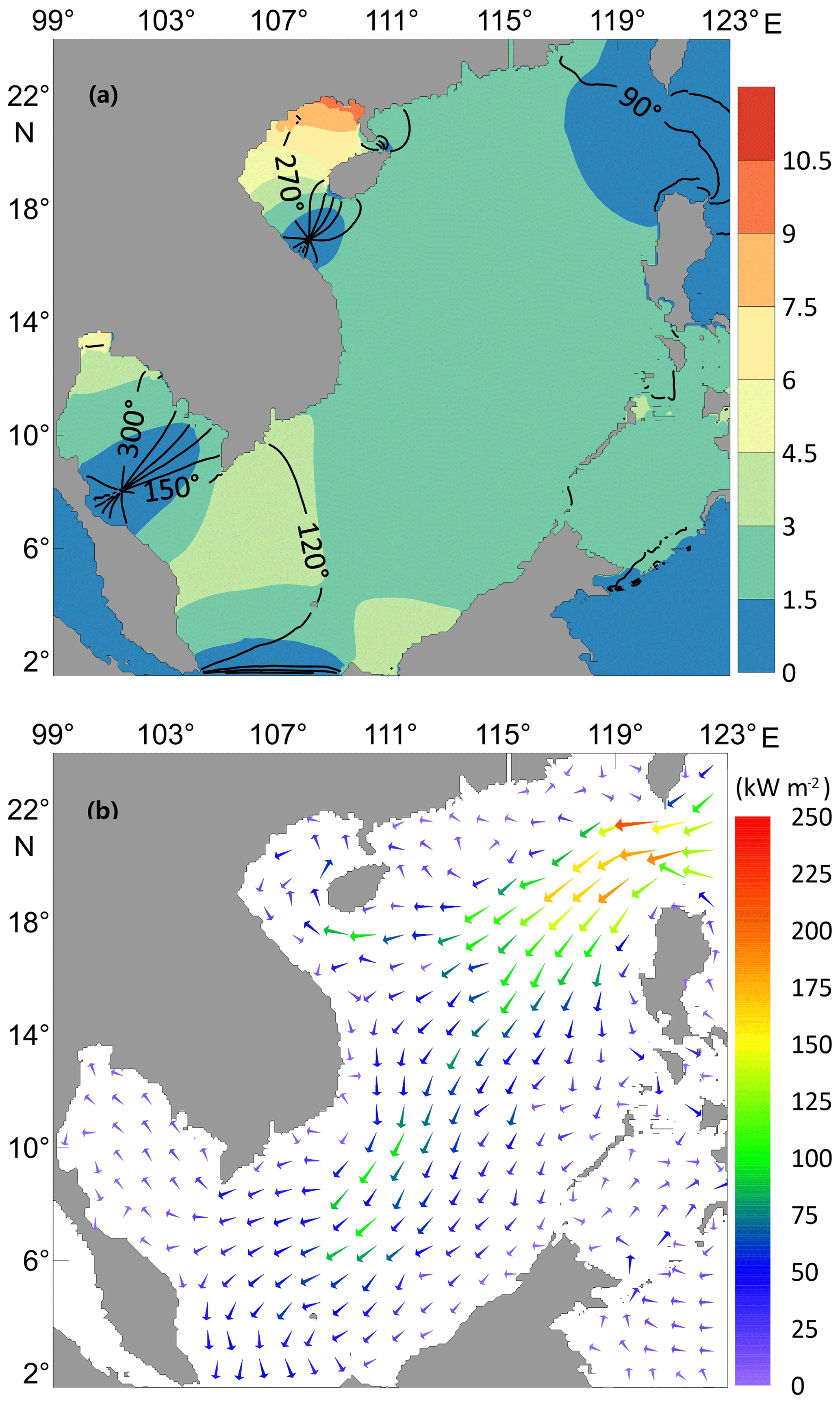
https://www.ocean-sci.net/15/321/2019/os-15-321-2019-f04

Figure 4(a) Distribution of amplitude gain (color) and phase change (lines in degrees) for the frequency of 0.99 cycles per day; (b) corresponding energy flux density vectors.

Download

Table 2Resonant frequencies and periods obtained from the six experiments.

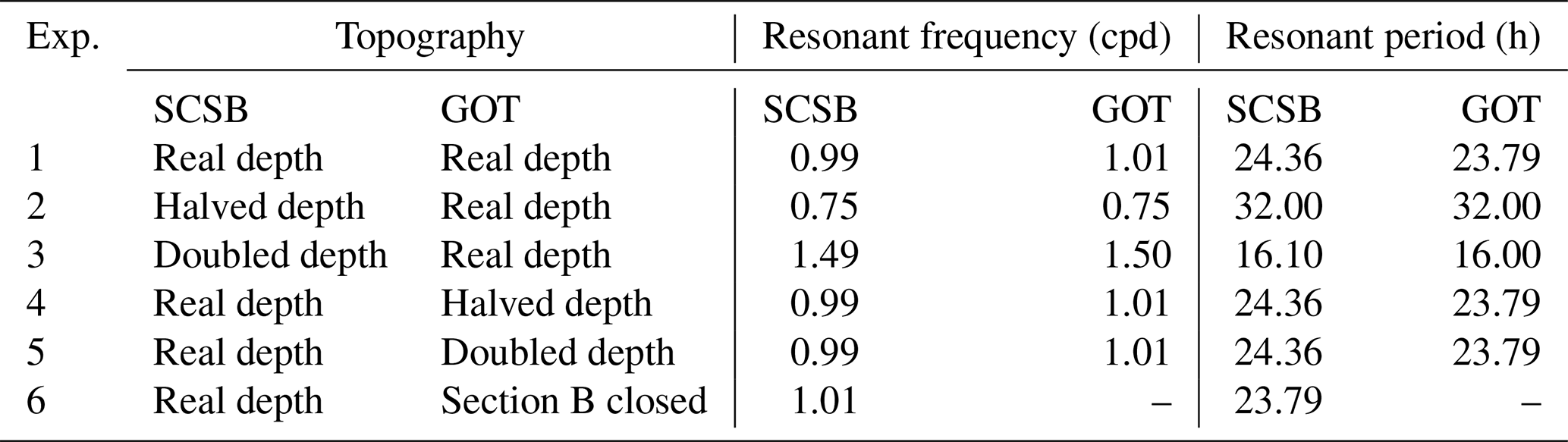
Download Print Version | Download XLSX

Table 2 and Fig. 3 show that when real water depths are used, the frequency corresponding to peak amplitude in the SCSB appears at 0.99 cpd, while that in the GOT is 1.01 cpd. The frequencies corresponding to peak amplitudes in the two areas are basically the same, and both are very close to that of the diurnal tide K₁, whose frequency is equal to 1.00 cpd (or more precisely, 1.0027 cpd). The spatial patterns of the amplitude gain and phase change for the frequency 0.99 cpd are displayed in Fig. 4a, with corresponding energy flux density vectors shown in Fig. 4b (the corresponding figures for 1.01 cpd are almost the same and are thus not shown). We can find that the patterns shown in Fig. 4 are quite similar to the simulated K₁ patterns shown in Fig. 2. Minor differences are caused by the use of different open boundary conditions.

From Fig. 3a, b, we can see that the peak amplitude gains in the GOT and SCSB are reduced when the depths of the SCSB are changed to half of the real depths. This reduction in amplitude gain occurs because friction increases as depth decreases (see Eqs. 2 and 3). Moreover, the amplitude peak frequencies in the GOT and SCSB both change to 0.75 cpd (Fig. 3a, b and Table 2), indicating that the resonant frequency in the GOT is determined by that of the SCSB. When the depths of the SCSB are doubled, the amplitude peak frequencies of the SCSB and GOT are increased to 1.49 and 1.50, respectively (Fig. 3a, b and Table 2), again indicating that the peak frequency of the GOT is determined by that of the SCSB. It is worth noting that when the depths in the SCSB are artificially changed by factors of 1∕2 and 2, the resonant frequencies are roughly changed by factors of $\sqrt{1 / 2}$ and $\sqrt{2}$ , respectively. This indirectly indicates that the quarter-wavelength resonance theory is applicable to the SCSB.

In Exp. 3, there is another weaker peak in the SCSB at the frequency of approximately 1.15 cpd (Fig. 3a). The peak frequency response may also have an effect on the GOT (Fig. 4b, Exp. 3), which results in a plateau peak of GOT between 0.5 and 1.2 cpd. This may be due to the deepening of the SCSB, resulting in discontinuity of topographic data at the junction with the GOT. Moreover, the amplitude gains in the GOT are significantly increased by increasing the depth, which results in reduced friction (see Eqs. 2 and 3).

Experiments 1–3 suggest that the peak response frequency of the GOT is strongly affected by the SCSB. Here, we conduct further experiments (Exps. 4–6) to investigate whether the GOT can also influence the resonance of the SCSB. From the results of Exps. 4–5 (Table 2, Fig. 3c, d), it can be seen that changing the depths of the GOT has little effect on the peak response frequencies of the SCSB and GOT. That is, the resonant frequencies of both areas are still close to one cycle per day.

In Exp. 6, the mouth boundary of the GOT (indicated by the blue B line in Fig. 1) is artificially closed. The results of this experiment show that the GOT has a small influence on the response of the SCSB, as shown in Fig. 3c. When boundary B is closed, the resonant frequency of the SCSB becomes slightly higher than the frequency of the K₁ tide, and the response amplitude of the SCSB in the vicinity of the resonant frequency is slightly reduced. As indicated by Arbic et al. (2009), when a shallow basin is connected to a deep basin, the impact of the shallow basin on the tidal response in the deep basin is determined by the depth ratio, width ratio and length ratio of these two basins as well as the friction in the shallow basin. In the present case, the depth and width ratios of the GOT against the SCSB are small, and tides in the GOT are strongly damped, so the impact of the GOT on the SCSB is not significant. In addition, there is a weak response peak at the frequency 0.45 cpd in the GOT (Exp. 1 in Fig. 3b). Since the GOT has a length of 660 km and a mean depth of 36 m, the quarter-wavelength theory gives a resonant frequency of 0.61 cpd. It seems that the peak at 0.45 cpd is associated with the local regional resonance.

In summary, the resonant periods or frequencies change when the depth of the SCSB varies, and the trends in the two sea areas are consistent (Fig. 3). The resonant frequency decreases when the SCSB is shallower and increases when the SCSB is deeper. Additionally, the resonant frequencies of the SCSB and GOT remain almost identical (Table 2). The experimental results show that the SCSB has a critical impact on the tidal response of the GOT and that the GOT is not an independent sea area in terms of tidal resonance.

https://www.ocean-sci.net/15/321/2019/os-15-321-2019-f05

Figure 5The two-channel model configuration representing the SCSB-GOT system.

Download

5 A theoretical model

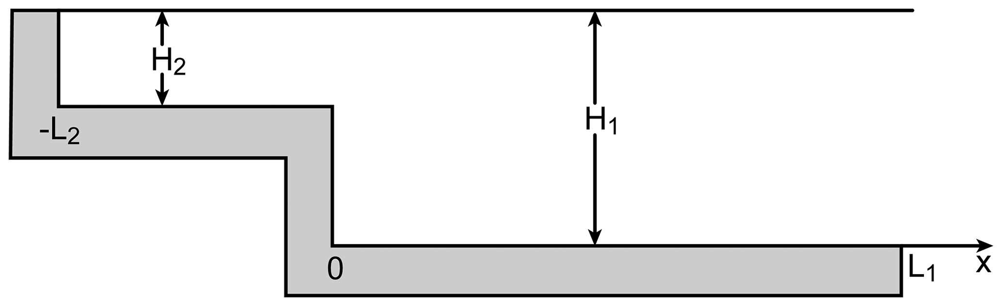
The quarter-wavelength resonant theory is based on the wave behavior in a single channel. As discussed above, this theory does not explain the enhanced tides around one cycle per day in the GOT. Here, we establish a two-channel model and examine its applicability to the SCSB-GOT system. Tidal waves from the Pacific Ocean propagate through the LS, pass the SCSB and finally enter the GOT. The tidal waves in the Karimata Strait are very weak (Fig. 2a and Wei et al., 2016) and are not able to propagate into the GOT. Thus, the tidal energy in the GOT is mainly from the SCSB. Therefore, we use a two-channel model to represent the SCSB-GOT system, as shown in Fig. 5. This model is quite similar to Webb's (2011) 1-D model, except that we add a forcing at the entrance of the deep channel. In the figure, H₁ is the depth of channel 1 (the deep channel), H₂ is the depth of channel 2 (the shallow channel), and L₁ and L₂ are the lengths of channels 1 and 2, respectively. The tidal waves enter channel 1 through the opening at x=L₁, enter channel 2 through the junction point at x=0 and finally reach the top of channel 2 at $x = - L_{2}$ . The equations governing the tidal motion in channels can be expressed as follows:

\begin{matrix} (7) & \{\begin{cases} \frac{\partial {\tilde{u}}_{m}}{\partial t} = - g \frac{\partial {\tilde{ζ}}_{m}}{\partial x} - γ_{m} {\tilde{u}}_{m} \\ \frac{\partial {\tilde{ζ}}_{m}}{\partial t} = - H_{m} \frac{\partial {\tilde{u}}_{m}}{\partial x}, \end{cases}, \end{matrix}

where ${\tilde{ζ}}_{m} (x, t)$ and ${\tilde{u}}_{m} (x, t)$ represent the elevation and velocity, respectively; H_m is the depth; γ_m is the friction parameter (equivalent to τ∕H in Eqs. 2 and 3); g is the acceleration due to gravity; and $m = 1, 2$ represents the different channel segments. Here, ${\tilde{u}}_{m} (x, t)$ and ${\tilde{ζ}}_{m} (x, t)$ can be expressed in the forms of ${\tilde{u}}_{m} (x, t) = R_{e} (u_{m} (x) e^{- i ω t})$ and ${\tilde{ζ}}_{m} (x, t) = R_{e} (ζ_{m} (x) e^{- i ω t}$ ), respectively, where ω is the angular frequency, t is time, and ζ_m(x) and u_m(x) represent the complex amplitudes of the elevation and velocity, respectively. By eliminating the common factor e^−iωt, Eq. (7) can be reduced to ordinary differential equations as follows:

\begin{matrix} (8) & \{\begin{cases} - i ω u_{m} = - g \frac{d ζ_{m}}{d x} - γ_{m} u_{m} \\ - i ω ζ_{m} = - H_{m} \frac{d u_{m}}{d x} . \end{cases} \end{matrix}

The boundary and matching conditions are as follows:

\begin{array}{l} (9) & ζ_{1} (L_{1}) = a_{0}, ζ_{1} (0) = ζ_{2} (0), \\ (10) & H_{1} u_{1} (0) = H_{2} u_{2} (0), \end{array}

and

\begin{matrix} (11) & u_{2} (- L_{2}) = 0 . \end{matrix}

From the governing equations and boundary/matching conditions, the complex amplitudes of the elevations of the two channels can be obtained as follows (see the Appendix for a detailed derivation):

\begin{matrix} (12) & ζ_{1} (x) = a_{0} R_{0} Q (x), \end{matrix}

and

\begin{matrix} (13) & ζ_{2} (x) = a_{0} R_{0} \cos β_{2} (x + L_{2}) . \end{matrix}

When the denominator of R₀ reaches its minimum, the amplitudes of the two-sea area become the largest and resonance occurs. The condition is as follows (see expression of R₀ in the Appendix, Eq. A10):

\begin{matrix} (14) & | \cos β_{1} L_{1} \cos β_{2} L_{2} - (r p_{1} / p_{2}) \sin β_{1} L_{1} \sin β_{2} L_{2} | = min, \end{matrix}

where $r = \sqrt{H_{2} / H_{1}}$ and $p_{m} = \sqrt{1 + i μ_{m}}$ .

https://www.ocean-sci.net/15/321/2019/os-15-321-2019-f06

Figure 6Response function at the locations $x = - L_{2}$ (a) and x=0 (b) with and without friction.

Download

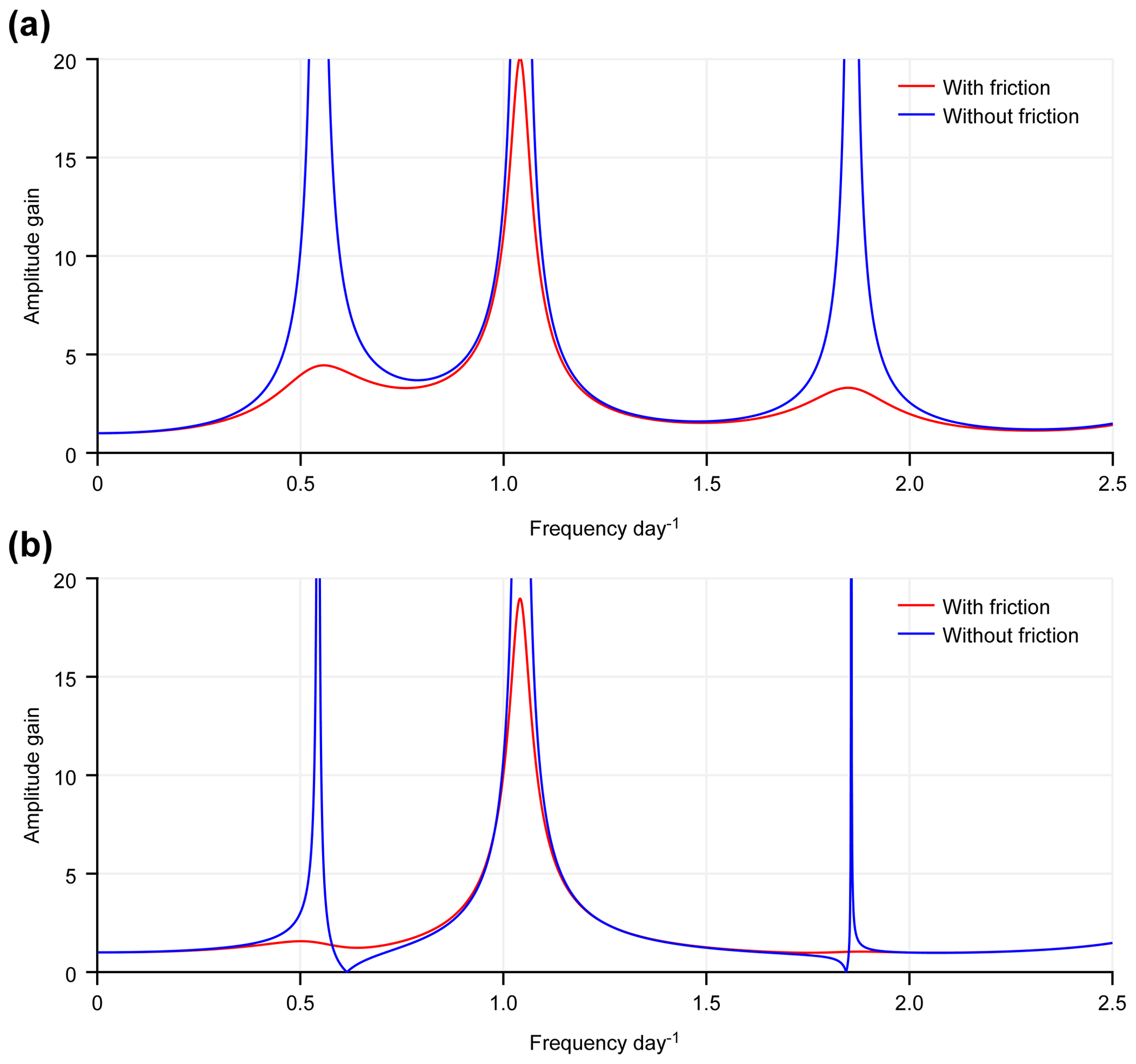
Based on the configurations of the SCSB and GOT, we take L₁=2600, L₂=660 km, H₁=1457, H₂=36 m, and $γ_{m} = \frac{0.0001}{H_{m}}$ . By substituting these values into Eqs. (12) and (13), we can obtain the solutions of these equations. The amplitude gains at locations x=0 and −L₂ are functions of ω or functions of the frequency f ( $f = ω / 2 π)$ and can be used to represent the response properties of channels 1 and 2, respectively. The results are shown with red curves in Fig. 6. For comparison, we also calculate the corresponding functions in the absence of friction, as shown by the blue curves in Fig. 6. From these curves, the resonant frequencies can be readily obtained, as given in Table 3.

Table 3The resonant frequencies and corresponding periods at $x = - L_{2}$ and $x = 0 .$

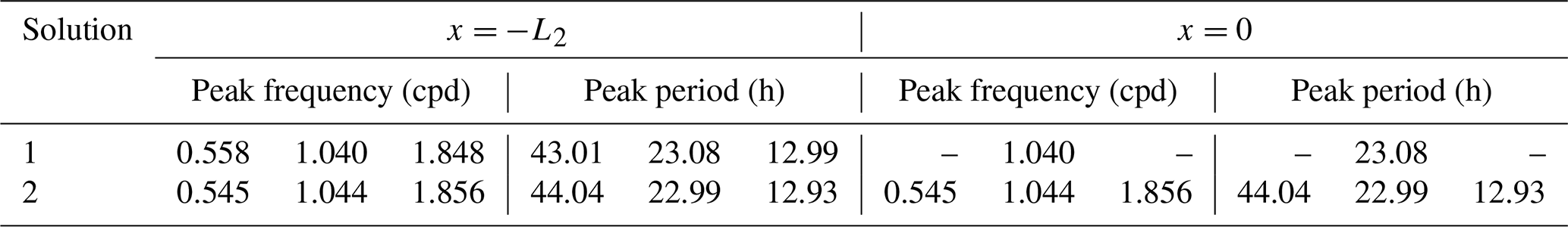
Solutions 1 and 2 are, respectively, for the cases in the presence and in the absence of friction.

Download Print Version | Download XLSX

Figure 6a displays the response function at $x = - L_{2}$ , which represents the response of channel 2. This figure shows that the results in the presence of friction are more realistic than those in the absence of friction. The former case has a maximum peak at a frequency of 1.040 cpd. The corresponding resonant period is 23.08 h, and this value is similar to the result of the numerical experiment involving the natural basin (Table 2, Exp. 1). The secondary response peak appears at a frequency of 0.558 cpd, which is also fairly consistent with the results for the natural basin, as shown in Fig. 3b (red curve). The third peak is very small and appears at a frequency of 1.848 cpd. If we carefully examine the red curve in Fig. 3b, we can also find a small peak near a frequency of 1.9 cpd. The response function is worse when friction is neglected than when friction is retained, but the obtained resonant frequencies are almost unchanged, as shown by the blue curve in Fig. 6a. Figure 6b shows the response function at x=0, which represents the response of channel 1. The red curve has only one peak at a frequency of 1.040 cpd, which is also similar to the results of the numerical experiment applied to the natural basin (Table 2, Exp. 1). When the friction is neglected, the frequency of the main peak is unchanged. In addition, there are two other peaks that are very narrow, indicating that these two peaks are relatively insignificant.

If we apply the quarter-wavelength resonance theory to channel 1, we can obtain resonant frequencies of 0.99 cpd. If we apply the quarter-wavelength and three-quarter-wavelength resonance theories to channel 2, we can obtain resonant frequencies of 0.61 and 1.84 cpd, respectively. Therefore, we can conclude that the major peaks around the frequency of 1.04 cpd in Fig. 6 are caused by resonance in channel 1. This indicates that channel 1 plays a determinative role in the two-channel system. Similarly, we can also conclude that the secondary and tertiary peaks around the frequencies of 0.55 and 1.85 cpd in Fig. 6 are caused by resonances in channel 2, associated with the quarter-wavelength and three-quarter-wavelength resonances. Although the frequencies of the peaks shown in Fig. 6 correspond well with those estimated based on the quarter-wavelength and three-quarter-wavelength theories, there are small discrepancies. This is due to the connection of the two channels. In fact, the resonant frequencies of the two-channel system also depend on the depth ratio of two channels, as shown in Eq. (14). In comparison to channel 2, the secondary, especially the tertiary peak, in channel 1 is much more less significant. This can be explained as follows: The tidal incident wave from the channel 1 partially enters channel 2 across the steep topography at x=0, and here, the rest of the wave is reflected. The reflected wave is superimposed with the incident wave, and tidal resonance occurs around the frequency of 1.04 cpd. That is, the steep topography at x=0 acts as a wall for channel 1, which causes the quarter-wavelength resonance to occur in the channel. Furthermore, the steep topography can also block most energy of the wave in channel 2 from entering channel 1. Therefore, the relatively large amplitudes in channel 2 at frequencies around 0.55 and 1.85 cpd are not obvious in channel 1 under the action of friction.

https://www.ocean-sci.net/15/321/2019/os-15-321-2019-f07

Figure 7The amplitude gain as a function of x for different peak frequencies with friction (a) and without friction (b).

Download

Figure 7 displays the amplitude gains along the channels when channel 2 is in a resonant state. The solution in presence/absence of friction is shown in Fig. 7a, b. The figure shows that when the forcing frequency is equal to 1.040 cpd, which is the major resonant frequency, the amplitude gain gradually increases from the mouth towards the head in channel 1. In channel 2, the amplitude gain decreases first and reaches a trough before increasing again towards the head. The trough corresponds with the amphidromic zone of the diurnal tides in the GOT (see Fig. 2a or the cotidal charts in Wu et al., 2015). For a frequency of 0.558 cpd, the amplitude gain is nearly constant in channel 1 and increases with a relatively high rate towards the head in channel 2. For a frequency of 1.848 cpd, the amplitude gain is also nearly constant in channel 1, and in channel 2, there are two antinodes and one node. This result is similar to the distribution of semi-diurnal tides in the GOT. When friction is neglected, the basic characteristics are the same but the amplitude gain significantly increases.

6 Conclusions

The GOT is dominated by diurnal tides, indicating that the response near the diurnal tide frequency in the GOT is stronger than that at other frequencies. However, when applied to the GOT, the classical quarter-wavelength resonant theory fails to yield a diurnal resonant period. Changing the water depths in the SCSB in our numerical experiments further shows that the resonance of the SCSB has a critical impact on the resonance of the GOT. An idealized two-channel model that can reasonably explain the resonance in the GOT is established. Through the numerical experiments and two-channel model, we found that the resonant frequency around one cycle per day in the South China Sea main area can be explained with the quarter-wavelength resonance theory, and the large-amplitude response at this frequency in the GOT is basically a passive response of the gulf to the increased amplitude of the wave in the southern portion of the main area of the South China Sea. However, there are still some problems that require further exploration, such as the effects of the length, width, depth, Coriolis force and friction of the SCSB on the GOT, which will be the focus of subsequent studies.

Code availability

In this paper, we use the Princeton Ocean Model (POM), which is available online at http://www.ccpo.odu.edu/POMWEB/ (Mellor, 2002).

Data availability

The ETOPO1 data (https://doi.org/10.7289/V5C8276M) came from NGDC, NOAA (https://www.ngdc.noaa.gov/mgg/global/, Amante and Eakins, 2009). The tidal data at the open boundaries came from the Oregon State University (ftp://ftp.oce.orst.edu/dist/tides, Egbert and Erofeeva, 2002.)

Author contributions

XC modified and ran the POM model, solved the analytical model, and prepared the draft of the manuscript. GF designed the method for numerically computing response functions and the configuration of the analytical model, and modified the manuscript. DW examined the derivation of the analytical solution.

Competing interests

The authors declare that they have no conflict of interest.

Acknowledgements

This study was supported by the National Key Research and Development Program of China (2017YFC1404200), the NSFC-Shandong Joint Fund for Marine Science Research Centers (grant no. U1406404) and the Basic Scientific Fund for National Public Research Institutes of China (grant no. 2015G02). The authors sincerely thank the topical editor, Neil Wells, for handling our manuscript. We also sincerely thank two referees for reviewing our manuscript. In particular, David Webb thoroughly reviewed our manuscript and provided many useful comments and suggestions, which were of great help in improving our study.

Edited by: Neil Wells
Reviewed by: David Webb and one anonymous referee

References

Amante, C. and Eakins, B. W.: Etopo1 1 arc-minute global relief model: procedures, data sources and analysis, National Geophysical Data Center, Marine Geology and Geophysics Division, 2009.

Arbic, B. K., Karsten, R. H., and Garrett, C.: On tidal resonance in the global ocean and the back-effect of coastal tides upon open-ocean tides, Atmos. Ocean., 47, 239–266, https://doi.org/10.3137/OC311.2009, 2009.

Aungsakul, K., Jaroensutasinee, M., and Jaroensutasinee, K.: Numerical study of principal tidal constituents in the Gulf of Thailand and the Andaman Sea, Walailak Journal of Science and Technology, 4, 95–109, 2011.

Cui, X., Fang, G., Teng, F., and Wu, D.: Estimating peak response frequencies in a tidal band in the seas adjacent to China with a numerical model, Acta Oceanol. Sin., 34, 29–37, https://doi.org/10.1007/s13131-015-0593-z, 2015.

Egbert, G. D. and Erofeeva, S. Y.: Efficient inverse modeling of barotropic ocean tides, J. Atmos. Ocean. Tech., 19, 183–204, 2002.

Fang, G., Kwok, Y.-K., Yu, K., and Zhu, Y.: Numerical simulation of principal tidal constituents in the South China Sea, Gulf of Tonkin and Gulf of Thailand, Cont. Shelf. Res., 19, 845–869, https://doi.org/10.1016/S0278-4343(99)00002-3, 1999.

Garrett, C.: Tidal resonance in the Bay of Fundy and Gulf of Maine, Nature, 238, 441–443, https://doi.org/10.1038/238441a0, 1972.

Godin, G.: On tidal resonance, Cont. Shelf. Res., 13, 89–107, https://doi.org/10.1016/0278-4343(93)90037-X, 1993.

Mellor, G. L.: Users guide for a three-dimensional, primitive equation, numerical ocean model, available at: http://www.ccpo.odu.edu/POMWEB/, Princeton University, Princeton, 2002.

Miles, J. and Munk, W.: Harbor paradox, Journal of the Waterways and Harbors Division, 87, 111–130, 1961.

Munk, W. H. and Cartwright, D. E.: Tidal spectroscopy and prediction, Philos. T. Roy. Soc. A, 259, 533–581, 1966.

Roos, P. C., Velema, J. J., Hulscher, S. J. M. H., and Stolk, A.: An idealised model of tidal dynamics in the North Sea: resonance properties and response to large-scale changes, Ocean Dynam., 61, 2019–2035, https://doi.org/10.1007/s10236-011-0456-x, 2011.

Sirisup, S. and Kitamoto, A.: An unstructured normal mode decomposition solver on real ocean topography for the analysis of storm tide hazard, in: Proceedings of the IEEE Oceans Conference, Yeosu, South Korea, 21–24 May 2012, 1–7, 2012.

Sutherland, G., Garrett, C., and Foreman, M.: Tidal resonance in Juan de Fuca Strait and the Strait of Georgia, J. Phys. Oceanogr., 35, 1279–1286, https://doi.org/10.1175/JPO2738.1, 2005.

Teng, F., Fang, G. H., Wang, X. Y., Wei, Z. X., and Wang, Y. G.: Numerical simulation of principal tidal constituents in the Indonesian adjacent seas, Adv. Mar. Sci., 31, 166–179, 2013.

Tomkratoke, S., Sirisup, S., Udomchoke, V., and Kanasut, J.: Influence of resonance on tide and storm surge in the Gulf of Thailand, Cont. Shelf. Res., 109, 112–126, https://doi.org/10.1016/j.csr.2015.09.006, 2015.

Webb, D. J.: Notes on a 1-D model of continental shelf resonances, Research and Consultancy Report 85, National Oceanography Centre, Southampton, 2011.

Webb, D. J.: On the tides and resonances of Hudson Bay and Hudson Strait, Ocean Sci., 10, 411–426, https://doi.org/10.5194/os-10-411-2014, 2014.

Wei, Z., Fang, G., Susanto, R. D., Adi, T. R., Fan, B., Setiawan, A., Li, S., Wang, Y., and Gao, X.: Tidal elevation, current, and energy flux in the area between the South China Sea and Java Sea, Ocean Sci., 12, 517–531, https://doi.org/10.5194/os-12-517-2016, 2016.

Wu, D., Fang, G., and Cui, X.: Tides and tidal currents in the Gulf of Thailand in a two-rectangular-Gulf model, Adv. Mar. Sci., 31, 465–477, 2013.

Wu, D., Fang, G., Cui, X., and Teng, F.: Numerical simulation of tides and tidal currents in the Gulf of Thailand and its adjacent area, Acta Oceanol. Sin., 37, 11–20, 2015.

Yanagi, T. and Takao, T.: Clockwise phase propagation of semi-diurnal tides in the Gulf of Thailand, J. Oceanogr., 54, 143–150, https://doi.org/10.1007/bf02751690, 1998.

Zu, T., Gan, J., and Erofeeva, S. Y.: Numerical study of the tide and tidal dynamics in the South China Sea, Deep Sea Res. Pt. I, 55, 137–154, https://doi.org/10.1016/j.dsr.2007.10.007, 2008.

Articles

Short summary

The resonant period of the Gulf of Thailand is potentially close to 1 day. However, the classic quarter-wavelength resonant theory fails to give a diurnal resonant period. In this study, we first perform a series of numerical experiments showing that the resonance of the South China Sea body has a critical impact on the resonance of the gulf. An idealised two-channel model that can reasonably explain the dynamics of the tidal resonance in the Gulf of Thailand is then established in this study.

Tidal resonance in the Gulf of Thailand

2.1 Governing equations and model configuration

2.2 Simulation of the K1 tide

3.1 Open boundary condition

3.2 Numerical model of the seas adjacent to China

2.2 Simulation of the K₁ tide