2.1 The wind-input source function

According to Du et al. (2017), the growth rate (β_g) of the WBLM wind-input source function $\left(S_{\text{in}}={\mathit{\beta }}_{\mathrm{g}}\left(\mathit{\sigma },\mathit{\theta }\right)N\left(\mathit{\sigma },\mathit{\theta }\right)\right)$ is expressed as

where N(σ,θ) is the action density spectrum, θ and θ_w are the wave and wind directions, C_β is the Miles parameter (Miles, 1957), ρ_w is the water density, and c is the phase velocity of waves. τ_t(z) is the local turbulent stress, which is equal to the total stress, τ_tot, minus the wave-induced stress, τ_w(z). The Miles parameter C_β is described as a function of the non-dimensional critical height, λ:

where κ=0.41 is the von Kármán constant, and J=1.6 is a constant. In Du et al. (2017), the expression of the non-dimensional critical height λ for Miles' parameter (Eq. 2) is derived by the assumption of a logarithmic wind profile following Janssen (1991), and it is expressed as

where g is the gravity acceleration, α=0.008 is a wave age tuning parameter according to Bidlot (2012), z₀ is the roughness length. However, it is found that using Eq. (3) causes numerical instability in some cases. This is because, within the WBL, the wind profile is not logarithmic under the impact of waves (Du et al., 2017). Using a logarithmic wind profile (Eq. 3) not only slows down the computation but could also fail in converging in some cases. Therefore, when applying WBLM S_in, the expression of λ also needs to be changed to adjust to the new wind profile. Here, we follow Miles (1957)'s procedure to drive an approximate expression for λ. In Miles (1957), the non-dimensional critical height is defined as

where k is the wave number, z_c is the critical height where the wave phase velocity (c) equals the wind speed component in the phase velocity direction $u\left(z_{\mathrm{c}}\right)\cdot \cos \left(\mathit{\theta }-{\mathit{\theta }}_{\mathrm{w}}\right)$,

where θ−θ_w is the angular separation between wind and wave directions. We assume that, in the vicinity of the critical height (z_c), the wind profile can be approximately described as locally logarithmic:

where $u_{*}^{\mathrm{l}}=\sqrt{{\mathit{\tau }}_{\mathrm{t}}/{\mathit{\rho }}_{\mathrm{a}}}$ is the local friction velocity. In the vicinity of the critical height, wind speed at any other heights z can be expressed as

where $z_{\mathrm{0}}^{\mathrm{l}}$ is a local effective roughness. Introducing Eqs. (7)–(5), we have wind speed at the critical height:

The critical height is calculated by combining Eqs. (7) and (8):

Considering the shallow-water dispersion relation, $k=(g/c^{\mathrm{2}})\tanh \left(kh\right)$, with h the water depth, the combination of Eqs. (4) and (9) results in the non-dimensional critical height for any direction:

It is found that Eq. (10) tends to underestimate wave growth at low frequencies. We used the same method as that used in WAM (Bidlot, 2012) and added a wave age tuning parameter (α=0.011) to shift the wave growth towards lower frequencies:

2.2 White-capping dissipation source function

The white-capping dissipation expression of KOM (Komen et al., 1984; Janssen, 1991; Bidlot et al., 2007) in SWAN is written as

where $\mathit{\varphi }\left(\mathit{\sigma },\mathit{\theta }\right)=\mathit{\sigma }N\left(\mathit{\sigma },\mathit{\theta }\right)$ is the frequency spectra. Since the WBLM wind-input and dissipation source functions are designed mainly for the wind sea, it is necessary to reduce the swell impact to the white-capping dissipation. In this study, the mean radian frequency 〈σ〉 and mean wave number 〈k〉 are modified according to Bidlot et al. (2007) to put more emphasis on the high frequencies:

where $m_{\mathrm{0}}=\int \int \mathit{\varphi }\left(\mathit{\sigma },\mathit{\theta }\right)\text{d}\mathit{\theta }\text{d}\mathit{\sigma }$ is the variance of the sea surface elevation. The choice of the two dissipation parameters, C_ds and Δ, is different for different wind-input source functions. For example, for KOM S_in, C_ds=2.5876 and Δ=1; for JANS S_in, C_ds=4.5, and Δ=0.5; for WBLM S_in in Du et al. (2017), Δ=0.1, and C_ds in S_ds is related to S_in to make sure

where

where U₁₀ is wind speed at 10 m, and $\stackrel{\mathrm{̃}}{E}=m_{\mathrm{0}}{g}^{\mathrm{2}}/U_{\mathrm{10}}^{\mathrm{4}}$ is a non-dimensional energy. As discussed in the introduction, a dissipation parameter that is strongly dependent on wind speed as in Eq. (12) only works in idealized fetch-limited cases but will in principle not work in real cases because wave breaking depends on wave state rather than wind. Here, we explore the use of some wave parameters to replace U₁₀ and S_in in Eqs. (11) and (12) to get rid of the direct dependence on wind speed. We derive the relationship between U₁₀, m₀, peak frequency (f_p), and fetch (x) from the three non-dimensional parameters, namely non-dimensional energy ($\stackrel{\mathrm{̃}}{E}$), non-dimensional peak frequency (${\stackrel{\mathrm{̃}}{F}}_{\mathrm{p}}=f_{\mathrm{p}}{U}_{\mathrm{10}}/g$), and non-dimensional fetch ($\stackrel{\mathrm{̃}}{x}=xg/U_{\mathrm{10}}^{\mathrm{2}}$). The fetch dependence of $\stackrel{\mathrm{̃}}{E}$ and ${\stackrel{\mathrm{̃}}{F}}_{\mathrm{p}}$ can be written as

where, in Kahma and Calkoen (1992) (composite condition), $A=\mathrm{5.2}\times {\mathrm{10}}^{-\mathrm{7}}$, B=0.9, C=2.1804, $D=-\mathrm{0.27}$. According to Eq. (12), U₁₀, $\stackrel{\mathrm{̃}}{E}$, and $\stackrel{\mathrm{̃}}{x}$ can be expressed as functions of m₀, f_p, and g:

where U₁₀, $\stackrel{\mathrm{̃}}{E}$, and $\stackrel{\mathrm{̃}}{x}$ are replaced by U^′, E^′, and x^′ since they are parameterized variables. The dissipation coefficient C_ds in Eq. (10) can be obtained by fitting the C_ds calculated from Eqs. (11) and (12) with U^′ and x^′ from Eq. (13):

The form and parameters in Eq. (14) will be obtained in the fetch-limited study in Sect. 4.1. To increase the robustness of the wave modeling in the case of unusual-shaped spectra, the peak frequency f_p in Eq. (13) is replaced by 0.866〈f〉 according to Komen et al. (1994) who uses k_p=0.75〈k〉, where $〈f〉=〈\mathit{\sigma }〉/\mathrm{2}\mathit{\pi }$ is the mean frequency. The use of 〈f〉 may cause uncertainty in estimating f_p, especially in, e.g., bimodal wave cases. Considering the model performs quite well during the two storm simulations in Sect. 4.3, during which bimodal waves probably exist, we assume that this uncertainty is relatively small.

To reduce the energy level at high frequencies, a cumulative term is added to the dissipation source functions. The cumulative dissipation term ($S_{\mathrm{ds}}^{\text{c}}$) follows Ardhuin et al. (2010), but the directional dependence of dissipation rate is not considered:

where C_cu=1.0 is a dissipation parameter, B_r=0.0012 is a saturation threshold, r_cu=0.5 is the ratio of the maximum frequency where dissipation of long waves influences short waves, C_g is the group velocity, and B(f) is the local saturation (van der Westhuysen et al., 2007):

2.3 Improvement of the numerical algorithm

Considering the expensive cost of WBLM code in Du et al. (2017), improvement of the numerical algorithm of the WBLM (Du et al., 2017) was done in the following aspects.

• The unnecessary calculations in the high frequencies were reduced. The WBLM uses 10 Hz as the maximum frequency, which is only being used for very young waves. Usually, the WBLM does not have to solve such high frequencies when the energy is so small that their contribution to the total wave-induced stress is negligible. Therefore, in the new code, the WBLM only solves the active frequency range which is dynamically changing with the wave spectrum. Although the maximum frequency is dynamically changing, all the active frequencies are solved, so there is no influence on the result. Such an adjustment reduces approximately half of the computation time in the idealized fetch-limited study in Sect. 3.1.

• The standard calculation in SWAN, a sweeping technique is used for the directional propagation of the waves, needs to be swept four times for each time step. Such a sweep is not necessary for the calculation of WBLM because the WBLM has to integrate over all directions of the spectra. Therefore, WBLM only calculates once per time step.

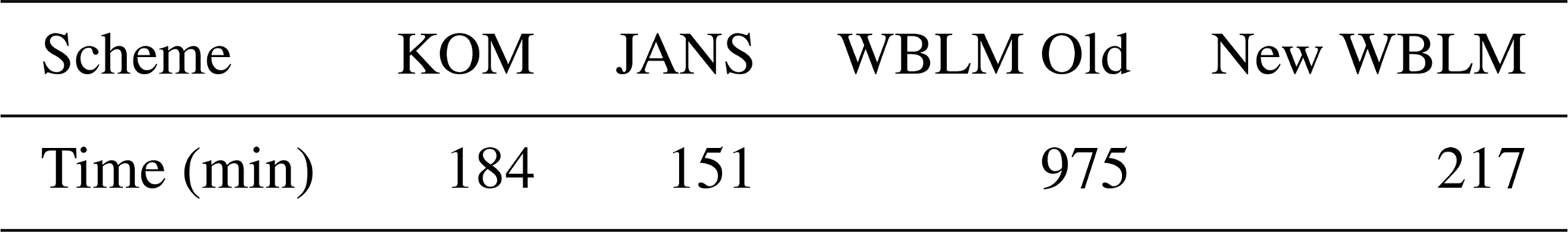
With the above mentioned refinement, the WBLM is now about 5 times faster than the previous version in Du et al. (2017). It is still slower than KOM and JANS, but it is fast enough for real applications. The averaged calculation time during an idealized fetch-limited study is listed in Table 1, including KOM, JANS, the previous WBLM of Du et al. (2017) (WBM Old), and the new WBLM in this paper. All the setups are the same as those in Sect. 3.1, except JANS uses frequency number ranges from 38 to 54 for different wind speed conditions, while the other schemes use 73 frequencies.

Table 1The calculation time of KOM, JANS, the previous WBLM of Du et al. (2017) (WBM Old), and the new WBLM during the idealized fetch-limited study.

Download Print Version | Download XLSX

3.1 Idealized fetch-limited study

The revised dissipation parameter (Eq. 14) in S_ds together with the new non-dimensional critical height as in WBLM S_in were first calibrated in the idealized fetch-limited wave growth experiments with the same model setup as in Du et al. (2017). Here, we briefly describe the model setup. We use the one-dimensional SWAN. The fetch is between 0 and 3000 km, with the spatial resolution changing gradually from 0.1 to 10 km. The wave spectrum ranges from 0.01 to 10.51 Hz, and the frequency discretization was logarithmic with a frequency exponent of 1.1, which results in 73 frequencies. We use 36 directional bins with a constant spacing of 10^∘. SWAN initializes from zero spectrum and runs for 72 h with a time step of 1 min. U₁₀ ranges from 5 to 40 ms⁻¹ and keeps constant during the 72 h simulation.

The calibration process is carried out in three steps. In Step 1, we run the model using the white-capping dissipation parameter as in Du et al. (2017) (Eqs. 11 and 12) in the idealized fetch-limited study. Since we added a cumulative dissipation source term, the parameters in Eq. (12) have to be changed into Eq. (16) so as to best fit to the Kahma and Calkoen (1992) fetch-limited wave growth curves:

In Step 2, the real form and parameters in Eq. (14) will be obtained by analyzing and fitting the C_ds with x^′ and U^′, which are calculated in Step 1. Finally, the best fit in Step 2 may not be the best choice for the wave model. Therefore, we selected several representative fitting parameters out of dozens of groups through idealized fetch-limited study as the final choice.

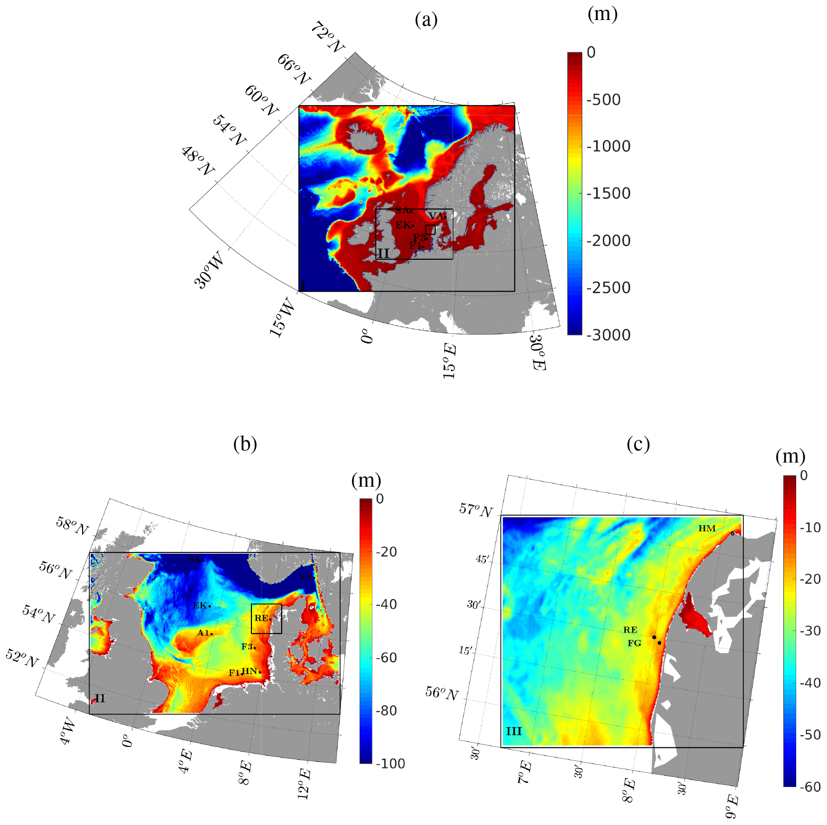
Figure 1SWAN domain for “Reducing the uncertainty of near-shore wind estimations using wind lidars and mesoscale models” (RUNE) storm simulation, with domains I at 9 km resolution, II at 3 km resolution, and III at 600 m resolution. Panels (a, b, c) show the bathymetry at domain I, II, and III. Bathymetry data are interpolated from EMODnet digital terrain model (DTM) 1∕8 arcmin data. The five measurement sites, RUNE (RE), Fjaltring (FG), Hanstholm (HM), A121 (A1), Väderöarna (VA), Heligoland north (HN), Fino-1 (F1), Fino-3 (F3), Sleipner-A (SA), and Ekofisk (EK), are shown as black dots.

Download

3.2 Idealized depth-limited study

In addition to the idealized fetch-limited study, the revised WBLM source terms are also tested in depth-limited wave growth experiments to check if the new source terms perform well with the interaction of the other source terms in the wave model, including the bottom friction and depth-induced wave-breaking dissipation source functions. Following SWAN (2014), we use JONSWAP (Hasselmann et al., 1973) bottom friction with a bottom friction coefficient, C_b=0.038 m² s⁻³, and Battjes and Janssen (1978) depth-induced wave-breaking source function with a breaker parameter, γ=0.8.

In the depth-limited wave growth experiments, we take the measurements of Young and Babanin (2006b) as reference for validation, because they not only provided detailed wind, wave, and water depth information but also provided wave spectrum measurement from capacitance wave probes up to 10 Hz (Young et al., 2005). Zijlema et al. (2012) conducted similar depth-limited wave growth experiments for the calibration of the bottom friction parameter in SWAN, but they did not compare the wave spectrum. Zijlema et al. (2012) selected 10 representative cases from the data presented in Young and Babanin (2006b). We add three more cases because the wave spectra in these three cases are also presented in Young and Babanin (2006b). This ends up with 13 cases in all, which are numbers 1, 11, 17, 23, 28, 30, 32, 58, 61, 63, 82, 83, and 87 in Table 1 of Young and Babanin (2006b). Among them, numbers 1, 11, 28, 32, and 87 have wave spectrum records for model validation. In all 13 cases, the water depth ranges from 0.89 to 1.1 m, and the wind speed ranges from 5.7 to 15 ms⁻¹. The fetch is set to 20 km with a spatial resolution of 0.1 km to ensure the fetch is long enough, and the wave growth is limited by the water depth. The frequency and directional discretization are same as those in the fetch-limited study. SWAN initializes from zero spectrum and runs for 24 h (we found 24 h is long enough for the wave development in the shallow-water conditions in this study), with a time step of 1 min. Two pairs of S_in and S_ds are tested, namely KOM (Snyder et al., 1981; Komen et al., 1984) and the revised WBLM in this study.

3.3 Real case study in the North Sea

The new WBLM S_in and S_ds are validated during two winter storms in the North Sea. Wind and wave measurements are obtained during the “Reducing the uncertainty of near-shore wind estimations using wind lidars and mesoscale models” (RUNE) project (Floors et al., 2016b). Simultaneous wind and wave measurements from lidar and buoys are available from November 2015 to January 2016. The experiment was conducted on the west coast of Jutland, Denmark, with an average water depth of 16.5 m. Details about the wind and wave measurements can be found in Floors et al. (2016b, a, c), Bolaños (2016), and Bolaños and Rørbæk (2016). Besides the standard wave parameters such as significant wave heights, peak wave period, and mean wave periods, the two-dimensional wave spectra E(f,θ) are also available, which allows us to validate more detailed aspects of the source functions. During the RUNE period, two storms passed the measurement site on 28 November 2015 and 12 August 2015. Wave simulations were done during this period with the three pairs of source terms (KOM, JANS, and WBLM). Besides the measurement from the RUNE project, point wave measurements at Fjaltring, Hanstholm, A121, Väderöarna, and Heligoland north from NOOS (https://noos.bsh.de/, last access: 15 June 2017) FINO-1 and FINO-3 from FINO (http://fino.bsh.de, last access: 3 April 2018) and Sleipner-A and Ekofisk from eKlima (http://sharki.oslo.dnmi.no, last access: 17 November 2016) during the simulation period are also used for model validation. The locations of these measurement sites are shown in Fig. 1a, b, and c.

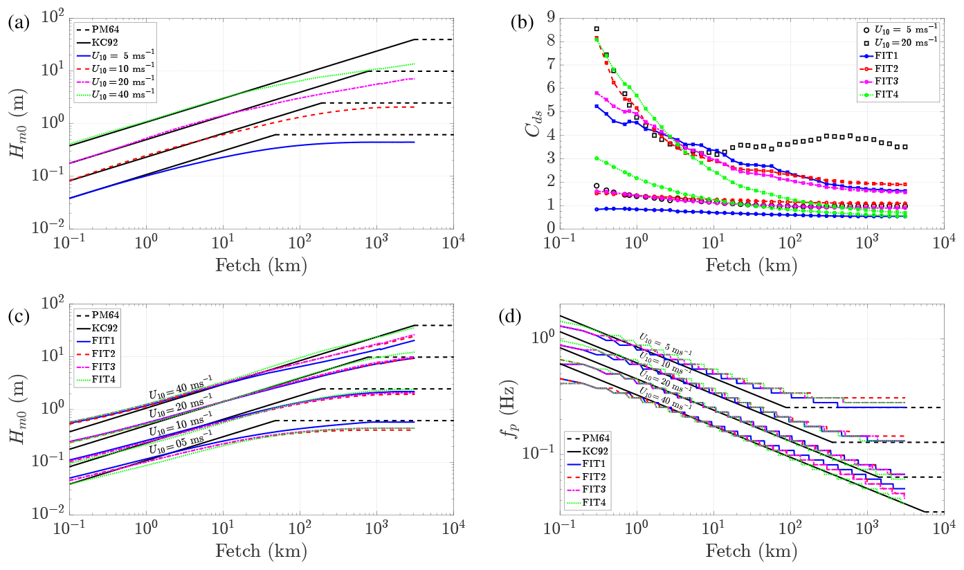
Figure 2H_m0 as a function of fetch after 72 h of simulation in different wind speed conditions using Eq. (16) as the white-capping dissipation parameter (a). C_ds as a function of fetch after 72 h of simulation in different wind speed conditions using Eq. (16), and fitted C_ds using FIT1 to FIT4 (b). H_m0 and f_p as a function of fetch using white-capping dissipation parameters from FIT1 to FIT4 (c, d).

Download

SWAN is forced by the National Centers for Environmental Prediction (NCEP) Climate Forecast System version 2 (CFSv2) 10 m wind (Saha et al., 2011). The quality of CFSv2 10 m wind speed and direction is evaluated with measurements in Fig. 6a–b, and it has been shown to be good quality for wave simulations in the North Sea in many previous studies (Bolaños et al., 2014). Therefore, the hourly CFSv2 data may be considered reasonable wind forcing, though it may not be accurate in the presence of highly fluctuating wind on scales smaller than 1 h, e.g., Larsén et al. (2017). SWAN uses three nested domains, with a resolution downscaling from 9 to 3 km and 600 m (Fig. 1a). Open boundaries for SWAN are set to 0. The shortest fetch of the observation points is larger than 1000 km according to the wind direction during the storm. According to the fetch-limited study in Sect. 4.1, the fetch is long enough for the waves to develop. The bottom friction and depth-induced wave-breaking source functions for the real case study are same as the depth-limited wave growth studies. Bathymetry data are obtained from the EMODnet digital terrain model (DTM) with a spatial resolution of 1∕8 arcmin. Note that most of the observations are located in the coastal areas in the North Sea, except Sleipner-A, A121, and Ekofisk (Fig. 1b, c). The water depth of most sites is less than 30 m, except Sleipner-A and Ekofisk, which are relatively deeper, with water depth around 80 and 60 m, respectively. SWAN initializes from zero spectrum, and the first 24 h output are not included in our analysis. The first storm peak is about 72 h after the model initializes to make sure the duration of the simulation is long enough. The frequency discretization was logarithmic with a frequency exponent of 1.1, and the lowest frequency was set to 0.03 Hz. For the KOM and WBLM source terms, a cut-off frequency of 10.05 Hz is used, giving a total of 61 frequencies; for JANS source terms, the cut-off frequency is set to 0.57 Hz to make sure the simulation is stable, giving a total of 31 frequencies. We used 36 directional bins and a 5 min time step. A summary of the constants and model setups used for all the experiments in Sect. 3 is given in Tables 2 and 3, respectively.

Table 2Constants used for all the experiments in Sect. 3. C_ds and Δ are white-capping dissipation parameters in Eq. (10); $F(x^{\prime },U^{\prime })$ is the new dissipation parameter for WBLM in Eq. (14); C_cu, B_r, and r_cu are cumulative dissipation parameter for WBLM in Eq. (15); C_b and γ are JONSWAP (Hasselmann et al., 1973) bottom friction and Battjes and Janssen (1978) depth-induced wave-breaking parameters.

Download Print Version | Download XLSX

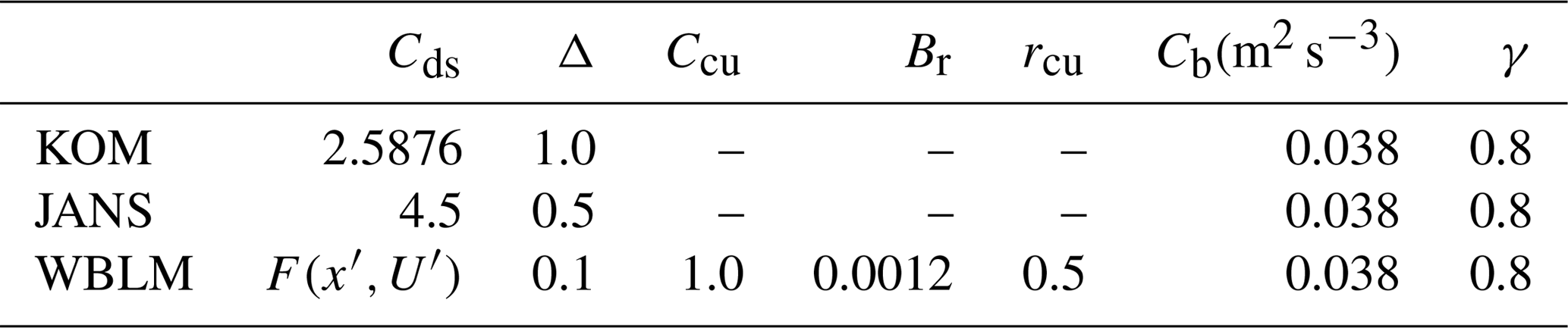
Table 3A summary of model setups for all the experiments in Sect. 3. dx is the spatial resolution and dt is the time step of SWAN in seconds.

Download Print Version | Download XLSX

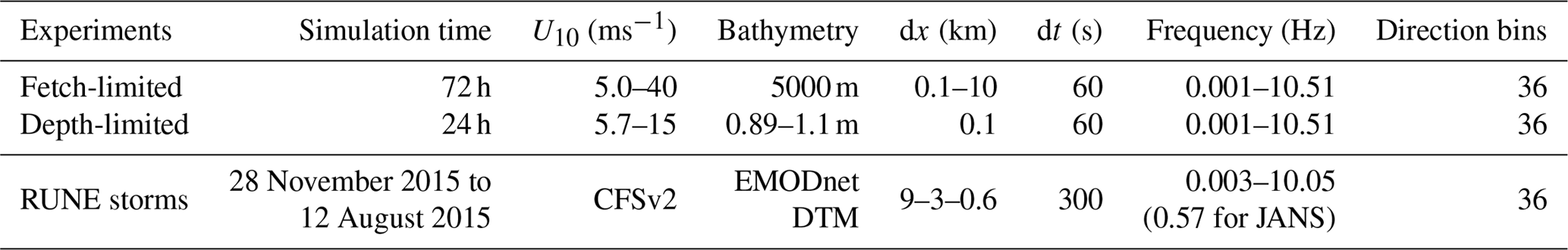
Figure 3Wave spectrum (a), wind-input and dissipation source terms (b), stress distribution over frequencies (c), and wind profile (d) calculated from WBLM, in 10 ms⁻¹ wind speed conditions at different fetches after 72 h simulation, in the fetch-limited wave growth study. The dashed lines and dotted lines in panel (a) are the wave spectrum parameterization from D85 (Donelan et al., 1985) and JONSWAP (Hasselmann et al., 1973); the solid lines are from WBLM. The solid, dashed, and dotted lines in panel (b) are the WBLM wind-input (S_in), white-capping dissipation (S_ds), and 5 times the cumulative dissipation ($\mathrm{5}{S}_{\mathrm{ds}}^{\mathrm{c}}$) source functions, respectively. Thick solid, thin solid, dashed, and dotted lines in panel (c) are the total stress (τ_tot), turbulent stress (τ_t), cumulative wave-induced stress (${\mathit{\tau }}_{\mathrm{w}}^{\mathrm{c}}$), and 5 times the local wave-induced stress ($\mathrm{5}{\mathit{\tau }}_{\mathrm{w}}^{\mathrm{l}}$) from WBLM. The solid lines in panel (d) are calculated from WBLM, and the dashed lines are the relative logarithm wind profiles extended from wind speed at 10 m elevation.

Download

4.1 Idealized fetch-limited study

The significant wave height (H_m0) calculated from Step 1 of the idealized fetch-limited study using Eqs. (11) and (16) is shown in Fig. 2a. The Kahma and Calkoen (1992) wave growth curves are also shown as solid black lines for reference. Note that Kahma and Calkoen (1992) curves come from data with limited wind speeds (U₁₀≤25 ms⁻¹) and fetches (x≤300 km), and we linearly extend them to broader ranges. The H_m0 calculated from Step 1 (solid colored lines in Fig. 2a) agrees with Kahma and Calkoen (1992) wave growth curves for fetches x≤10 km. But it tends to underestimate H_m0 for fetches x>10 km. Therefore, in Step 2, we only fit the C_ds in the first 10 km and extend its application for longer fetches. The C_ds calculated from Step 1 for wind speed U₁₀=5 ms⁻¹ and U₁₀=20 ms⁻¹ is shown in Fig. 2b as black circles and black rectangles. Here, we try to speculate the form of Eq. (14) based on the distribution of C_ds from Step 1 in Fig. 2b. First, C_ds has a clear dependence on U₁₀. We found that in 10 ms⁻¹ wind speed conditions, the simulated H_m0 follows the Kahma and Calkoen (1992) curves quite well in all fetches, while in the other wind speed conditions, the model underestimates H_m0 when U₁₀<10 ms⁻¹ or overestimates H_m0 when U₁₀>10 ms⁻¹. Therefore, we take 10 ms⁻¹ as reference, and there should be a $\left(\frac{U^{\prime }}{\mathrm{10}}\right)$ term in the C_ds equation. Second, C_ds depends on the fetch; considering the fetch dependence is logarithmic (the horizontal coordinate of Fig. 2b is logarithmic), there should be a ln(x) term in the C_ds equation. Considering that a log-transformed quantity must be unitless, we use the non-dimensional fetch ln(x^′) instead of ln(x). Therefore, we assume C_ds in Eq. (14) has the following form:

where C1, C2, C3, and C4 are parameters to be determined by fitting the C_ds calculated from Step 1. Directly using the four parameters may be easier to fit, but it requires more effort to use or change it in real applications. Therefore, instead of finding a random combination of the four parameters that gives the least square error, we prefer to reduce the number of fitting parameters based on our understanding of the role of the two terms, namely ln(x^′) and $\left(\frac{U^{\prime }}{\mathrm{10}}\right)$ in Eq. (16). We use fixed value for the power on ln(x^′) and $\left(\frac{U^{\prime }}{\mathrm{10}}\right)$. By testing $\mathrm{1}\le C\mathrm{2}\le \mathrm{4}$ with a resolution of 1, and $\mathrm{0}\le C\mathrm{4}\le \mathrm{1}$ with a resolution of 0.1, we choose C2=2 and 4, C4=0.5 and 1 as representative values. With the values of C2 and C4 provided, we fit C1 and C3 with the data from Step 1 and end up with the first three groups of fitting parameters listed in Table 4 (FIT1 to FIT3). FIT4 in Table 4 is an improvement for FIT3 which will be described latter. The fitted C_ds using FIT1 to FIT4 at different wind speed conditions is shown in Fig. 2b as colored lines with circles and rectangles representing wind speed.

Table 4Four groups of fitting parameters (FIT1, FIT2, FIT3, and FIT4) for Eq. (16).

Download Print Version | Download XLSX

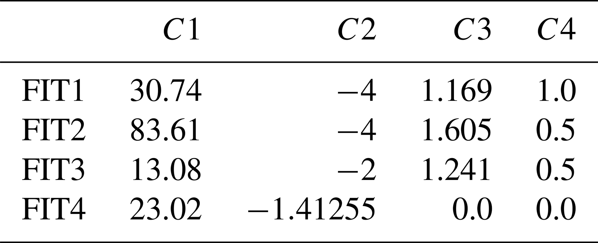
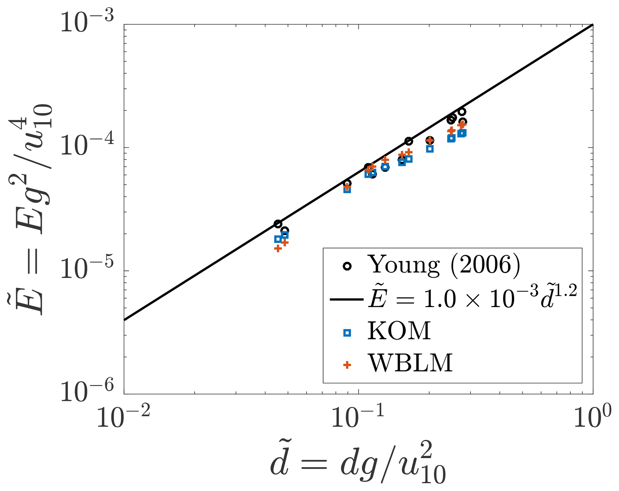
Figure 4Observed (black circles) and parameterized (black line) non-dimensional wave energy for fully developed waves in shallow water as a function of non-dimensional depth (Young and Babanin, 2006b) and SWAN results with KOM (blue squares) and WBLM (red crosses) source terms after 24 h simulation.

Download

The four groups of parameters (FIT1 to FIT4 in Table 4) are applied in SWAN in the fetch-limited study, and the results are shown in Fig. 2c, d. The effect of the ${\left(\frac{U^{\prime }}{\mathrm{10}}\right)}^{C\mathrm{4}}$ term in Eq. (16) can be seen from the comparison between FIT1 and FIT2. The fitted C_ds, simulated H_m0, and f_p of FIT1 and FIT2 are shown in Fig. 2b, c, d as blue solid and red solid lines with circles and rectangles representing wind speed. Although significant difference of C_ds between C4=1.0 (FIT1) and C4=0.5 (FIT2) is seen in Fig. 2b, the resulting H_m0 and f_p show a relatively small difference. In low wind speed conditions (U₁₀=5 and 10 ms⁻¹), C4=1.0 (blue solid lines in Fig. 2c, d) results in larger H_m0 (smaller f_p) than C4=0.5 (red solid lines in Fig. 2c, d). In high wind speed conditions (U₁₀=20 and 40 ms⁻¹), C4=1.0 underestimates H_m0 (overestimates f_p) more than C4=0.5 in long fetches (x>10 km).

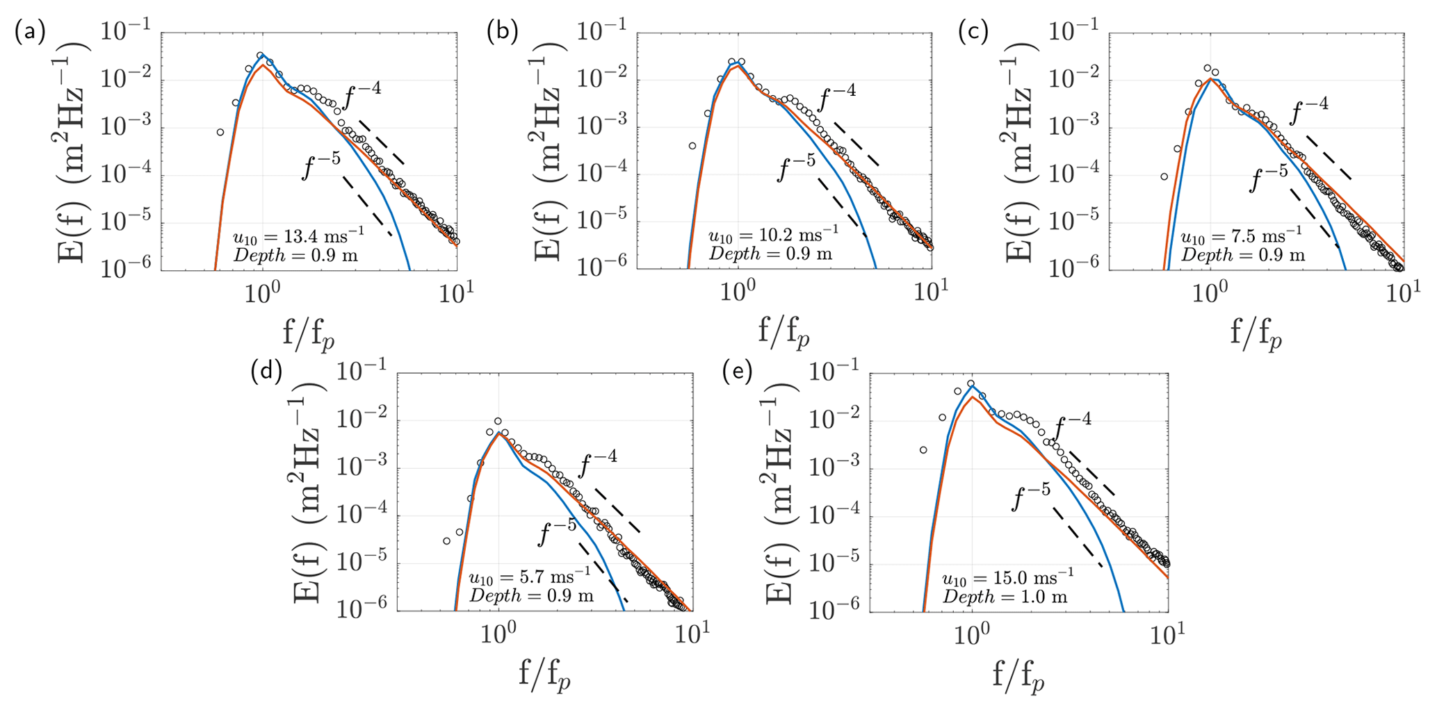
Figure 5One-dimensional wave spectrum measured by (Young and Babanin, 2006b) (black circles) for fully developed waves in shallow water and the results from SWAN with KOM (blue lines) and WBLM (red lines) source functions after 24 h simulation.

Download

The effect of the ln(x^′)^C2 term can be seen from the comparison between FIT2 and FIT3, the red solid and magenta dashed lines in Fig. 2b, c, d. The impact of C2 to H_m0 and f_p is much weaker than C4. Using C2=2 (magenta dashed lines in Fig. 2c, d) results in slightly larger H_m0 (smaller f_p) than C2=4 (red solid lines in Fig. 2c, d) in long fetches (x>10 km), which results in larger white-capping dissipation, smaller H_m0, and larger f_p.

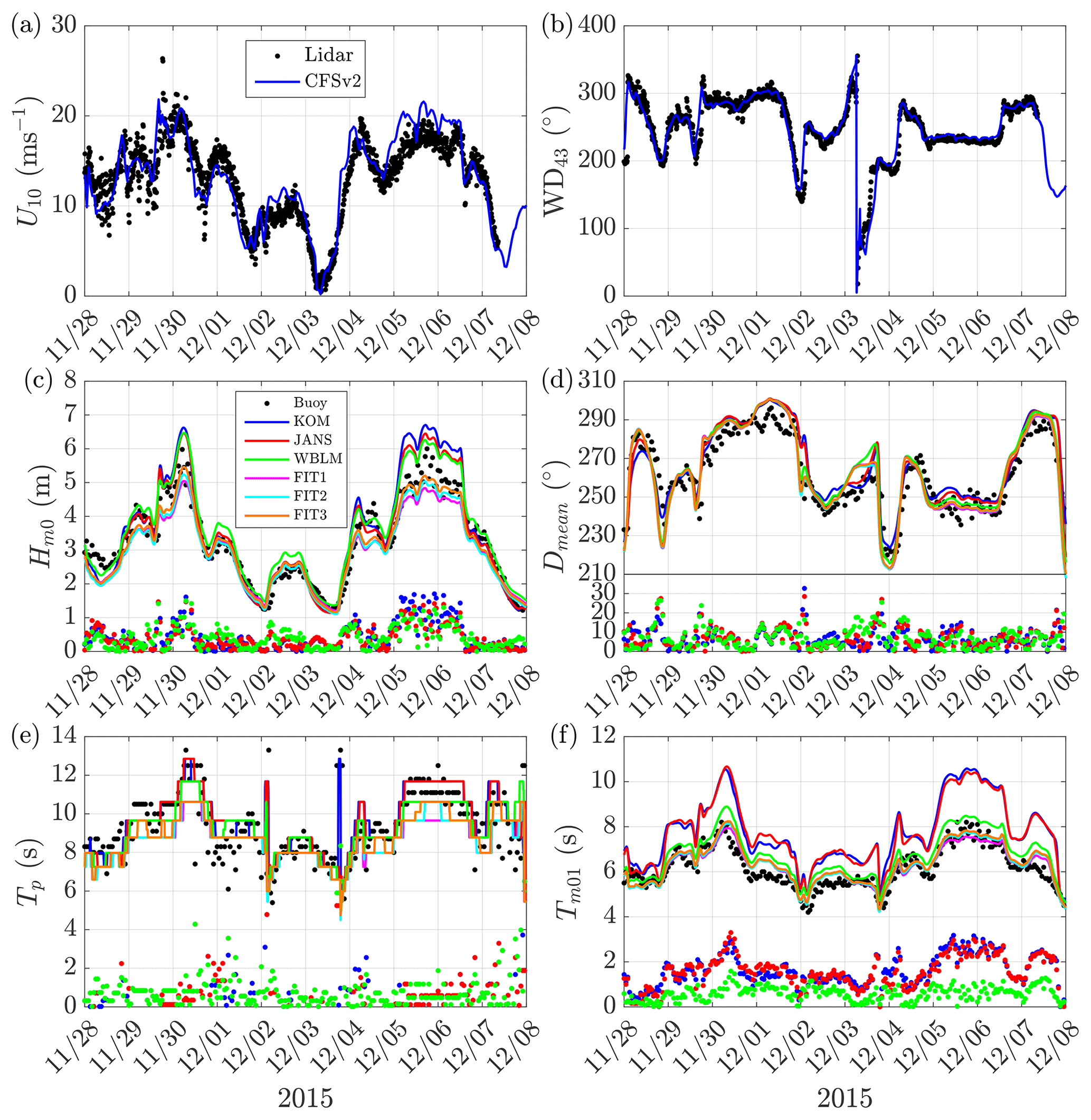
Figure 6Time series during two winter storms in the RUNE project. (a) The 10 m wind speed from CFSv2 and measurements calculated from a logarithm wind profile from lidar measurements at 43, 50, 62, 82, and 100 m. (b) Wind direction from CFSv2 and lidar measurement at 43 m. (c) Modeled significant wave height (solid lines) in comparison to buoy measurements (black dots); colored dots show the absolute error. (d) Mean wave direction. (e) Peak wave period. (f) Mean wave period.

Download

FIT1–FIT3 tend to underestimate H_m0 (overestimate f_p) in long fetches (x>10 km). In the real case study in Sect. 4.3, it will be shown that such an underestimation of H_m0 failed in capturing large waves in real storm simulations. Therefore, we continuously reduce the value of C2 and C4 until the large waves are captured in both the idealized fetch-limited study and real case study, which results in the parameters of FIT4 (hereafter WBLM). In FIT4, C4=0.0 means that $\left(\frac{U^{\prime }}{\mathrm{10}}\right)$ term is disappeared in Eq. (16). From Eq. (13), we found that both U^′ and x^′ could be written in the form of $A_{\mathrm{1}}{m}_{\mathrm{0}}^{A_{\mathrm{2}}}{f}_{\mathrm{p}}^{A_{\mathrm{3}}}$, which indicate that the function of the U^′ term could be replaced by changing the parameters in the x^′ term. This can be seen from the green lines in Fig. 2b that, without the $\left(\frac{U^{\prime }}{\mathrm{10}}\right)$ term, C_ds still follows different curves in different wind speed conditions.

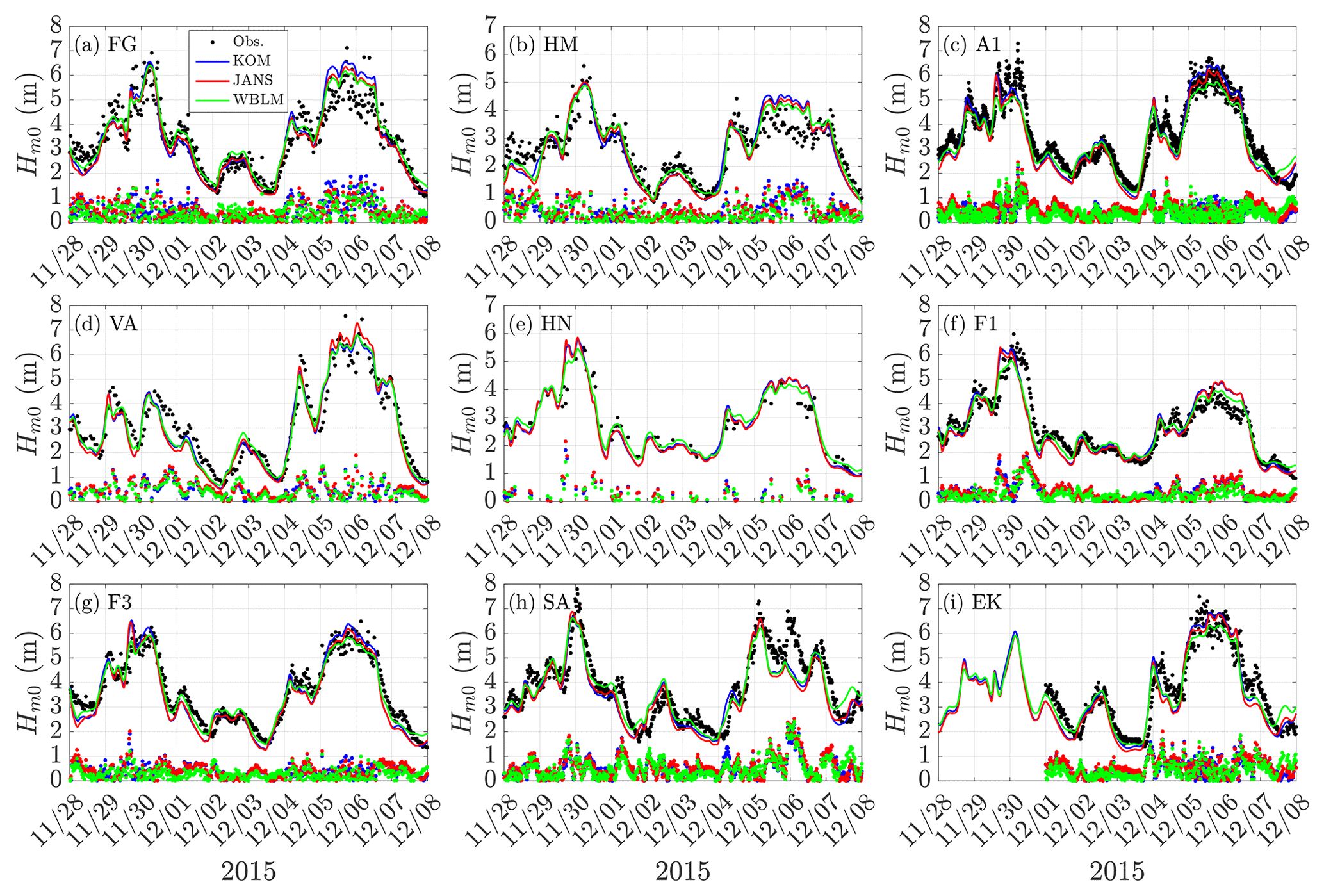
Figure 7Time series of H_m0 at Fjaltring (FG), Hanstholm (HM), A121 (A1), Väderöarna (VA), Heligoland north (HN), Fino-1 (F1), Fino-3 (F3), Sleipner-A (SA), and Ekofisk (EK) during the two winter storms in the RUNE project. Observations are shown in black dots, modeled H_m0 using different source terms are shown in colored solid lines, and the corresponding colored dots show the absolute error between modeled results and observations.

Download

Figure 3a shows the wave spectrum from WBLM (solid lines) in 10 ms⁻¹ wind speed conditions after 72 h simulation in comparison to the spectrum parameterization of D85 (Donelan et al., 1985) (dashed lines) and JONSWAP (Hasselmann et al., 1973) (dotted lines) with the fetch dependence from Kahma and Calkoen (1992). Detailed equations for D85 and JONSWAP are listed in Appendix Appendix A. The results from the WBLM source term generally follow the shape of the D85 and JONSWAP spectra, but they tend to underestimate the energy at low frequencies at fetches x≥10 km.

Figure 8One-dimensional wave spectrum from buoy measurements at RUNE with all available data during the two storms (a); panels (b–d) are simulated with different source terms. The colors of the lines represent different times. The black solid lines in each panel are the envelope lines to mark the upper and lower bounds of the measurement data.

Download

The D85 spectra at short fetches (e.g., 1 km) have less energy at high frequencies (e.g., f>1 Hz) than at long fetches (e.g., 3000 km). On the contrary, JONSWAP and WBLM spectra have more energy at short fetches than at long fetches at high frequencies. The D85 spectra have a f⁻⁴ shape at high frequencies, while JONSWAP has a f⁻⁵ shape. The high-frequency part of WBLM spectra is between f⁻⁴ and f⁻⁵. Figure 3b shows the source term distribution of wind-input (S_in, solid lines), white-capping dissipation (S_ds, dashed lines), and 5 times the cumulative dissipation ($\mathrm{5}{S}_{\mathrm{ds}}^{\text{c}}$, dotted lines) source functions at different fetches indicated by color legends in Fig. 3a. $\mathrm{5}{S}_{\mathrm{ds}}^{\text{c}}$ instead of $S_{\mathrm{ds}}^{\text{c}}$ is used to better visualize the cumulative dissipation source term. As the waves grow older, the S_in values at high frequencies become smaller, and $S_{\mathrm{ds}}^{\text{c}}$ values become larger, which may explain why the WBLM spectra have more energy at short fetches than at long fetches at high frequencies. Figure 3c shows the corresponding stress distribution within the wave boundary layer. Here, we also use $\mathrm{5}{\mathit{\tau }}_{\mathrm{w}}^{\mathrm{l}}$ (dotted lines) instead of ${\mathit{\tau }}_{\mathrm{w}}^{\mathrm{l}}$ for the purpose of visualizing the local wave-induced stress. Short fetch waves contribute more surface stress than long fetch waves at high frequencies, while they contribute less stress than long fetch waves at low frequencies. The total wave-induced stress depends on the integration of ${\mathit{\tau }}_{\mathrm{w}}^{\mathrm{l}}$ at all frequencies, which results in waves with a fetch of 5–15 km having the highest total wave-induced stress, waves with a fetch of 1 km having lower total wave-induced stress, and waves with a fetch of 3000 km having the lowest wave-induced stress. Accordingly, total wind stress (τ_tot, thick solid lines) at 5–15 km is larger than that at 1 and 3000 km because of the impact of the waves. Figure 3d shows the wind profiles within the wave boundary layer calculated by WBLM. Wind profiles are rather different in different wave development stages, which reveals that it is necessary to take the wave-induced wind profile variation into account in the estimation of the critical height in Sect. 2.1.

4.2 Idealized depth-limited study

Figure 4 shows the non-dimensional wave energy as a function of non-dimensional depth for fully developed waves in shallow waters after 24 h simulation, with the measurements of Young and Babanin (2006b) as reference. In comparison, results from KOM source terms are also shown. Both the WBLM (red crosses) and KOM (blue squares) show close agreement with the measurements (black circles).

The one-dimensional wave spectrum in the depth-limited experiment is further examined after 24 h simulation in Fig. 5a–e for different wind speed and depth conditions, with the measurements of Young and Babanin (2006b) as reference. Both models capture the peak of the wave spectrum. However, KOM (blue lines) tends to underestimate the energy level at high frequencies. On the contrary, the energy level of WBLM (red lines) at high frequencies closely follows the measurements.

4.3 Two storms during the RUNE project

During the two RUNE storms on 28 November 2015 and 12 August 2015, wave simulation was done with SWAN forced by CFSv2 wind. The performance of KOM, JANS, and WBLM source terms are evaluated with buoy measurements in terms of significant wave height H_m0, mean wave direction D_mean, peak period T_p, mean period T_m01, and one-dimensional wave spectrum. Figure 6 shows the simulated time series of H_m0, D_mean, T_p, and T_m01 in comparison to buoy measurements at RUNE. To see the impact of different parameters of the WBLM white-capping dissipation source function to the wave simulation, results from FIT1 to FIT3 are also shown. Similar to the conclusions in the idealized fetch-limited study in Sect. 4.1, these parameters significantly underestimate high waves. Only FIT4 (here WBLM) can be used for real wave simulations to capture the high waves.

Table 5Statistics of simulated significant wave height (H_m0), mean wave direction (D_mean), and peak (T_p) and mean (T_m01) wave period in comparison to buoy measurements at the RUNE site on 28 November 2015 and 12 August 2015. The statistics include mean difference (bias), root mean square error (RMSE), and scatter index (SI). In each column, the values of smallest absolute errors are indicated with bold text.

Download Print Version | Download XLSX

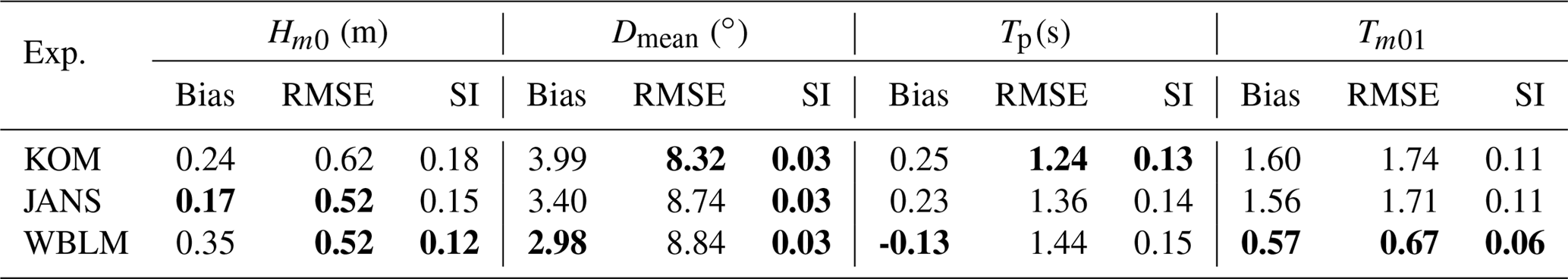
Now we compare the performance of the new WBLM with KOM and JANS source terms. For H_m0, D_mean, and T_p, all the modeled time series generally follow the general trends of measurement data. The biggest error of H_m0 happens at the two storm peaks. The three source terms overestimate the H_m0 during the peak at about 1 m (15 %). WBLM gives slightly better H_m0 during the peak than KOM and JANS. But it tends to underestimate T_p during the storm peaks. WBLM predicts T_m01 significantly better than KOM and JANS. Note that the buoy T_m01 is calculated from the frequency range of 0.005 to 0.64 Hz, JANS is from 0.03 to 0.58 Hz, and KOM and WBLM are from 0.03 to 0.63 Hz. A summary of the statistics is listed in Table 5, and the definitions of the statistics are given in Appendix Appendix B. WBLM generally provides better results for H_m0 and T_m01 than KOM and JANS. All the three source terms have similar accuracy in predicting D_mean. WBLM is slightly less accurate in predicting T_p than KOM and JANS.

Table 6Statistics of simulated significant wave height (H_m0) in comparison to measurements at Fjaltring (FG), Hanstholm (HM), A121 (A1), Väderöarna (VA), Heligoland north (HN), Fino-1 (F1), Fino-3 (F3), Sleipner-A (SA), and Ekofisk (EK) on 28 November 2015 and 12 August 2015. The statistics include mean difference (bias), root mean square error (RMSE), and scatter index (SI). In each column, the values of smallest absolute errors are indicated with bold text.

Download Print Version | Download XLSX

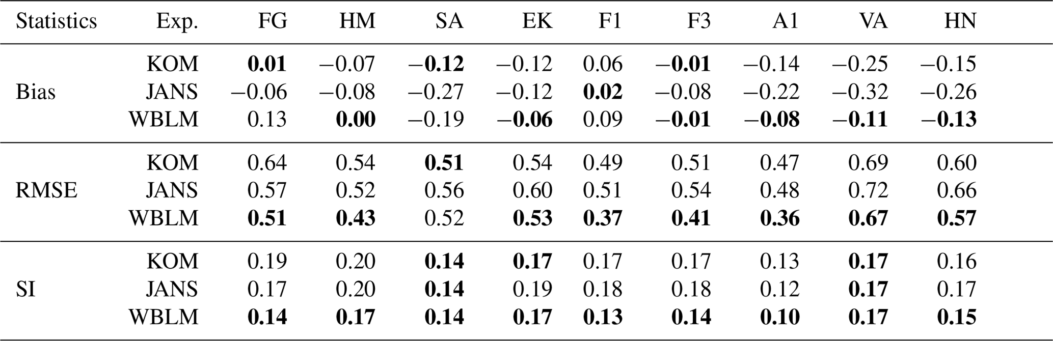
The time series of H_m0 at another nine measurement sites, including Fjaltring (FG), Hanstholm (HM), A121 (A1), Väderöarna (VA), Heligoland north (HN), Fino-1 (F1), Fino-3 (F3), Sleipner-A (SA), and Ekofisk (EK) in the North Sea during the two storm simulations, are shown in Fig. 7. The relative statistics are listed in Table 6. Considering the statistics of mean difference (bias), root mean square error (RMSE), and scatter index (SI), WBLM generally gives better H_m0 than KOM and JANS for most of the sites. However, in contrast to RUNE, WBLM tends to underestimate the largest waves during storm peaks in the open-ocean sites, e.g., the storm peak at A121 (Fig. 7c), Sleipner-A (Fig. 7g), and Ekofisk (Fig. 7i).

The one-dimensional wave spectrum during the whole simulation period at the RUNE site is presented in Fig. 8. The colored lines in Fig. 8a show the data from buoy measurements, and the black envelope lines are used to mark the upper and lower bounds of the measurement data. The colored lines in Fig. 8b, c, d are from SWAN simulations using KOM, JANS, and WBLM source terms, and the black envelope lines are the same as those in Fig. 8a. The three simulations generally capture the shape of the measured spectrum. In comparison to the measurements, KOM and JANS tend to overestimate the energy around the spectral peak, while WBLM gives better energy estimation around the spectral peak. Both KOM and JANS show a leveling off of energy at frequencies higher than about 0.3 Hz, while the measurement and WBLM do not, which may explain the failure of KOM and JANS in simulating T_m01. However, seemingly WBLM tends to overestimate the energy at frequencies higher than the peak, which needs further investigation.