2.1 Ensemble model simulation

Our example application is based on a $\mathrm{1}/\mathrm{4}{}^{\circ }$ resolution model of the North Atlantic and the Nordic Seas. We used the oceanic model NEMO (Madec, 2008) version 3.6, with the CREG4 configuration as part of the CMEMS project. NEMO, used by a large community, is developed by European institutes and is used by the majority of the CMEMS stakeholders. It is a primitive equation model which computes the following prognostic variables: 3-D velocities, sea surface height, salinity and temperature. ERA-Interim reanalysis data, produced at ECMWF (Dee et al., 2011), are used for the atmospheric forcing. CREG4 is a realistic configuration for the North Atlantic and the Nordic Seas at the $\mathrm{1}/\mathrm{4}{}^{\circ }$ horizontal resolution. This configuration is described in the work of Dupont et al. (2015), except that we use a $\mathrm{1}/\mathrm{4}{}^{\circ }$ version instead of the nominal $\mathrm{1}/\mathrm{12}{}^{\circ }$ resolution. It has been developed by Environment Canada and coupled with Mercator Océan's SAM2 data assimilation system. The aim was to build a realistic description of the mean state and variability in the North Atlantic and the Nordic Seas. The CREG4 configuration is currently used by Mercator Océan and its resolution is sufficient to evaluate the multiscale assimilation algorithm; therefore, we use it for our study.

Uncertainties in the model are explicitly simulated using the standard NEMO stochastic parameterisation module developed by Brankart et al. (2015). The aim is to produce an ensemble with a sufficient spread for all variables, especially for the observed variables, all over the domain. This technique has been used to simulate six different kinds of uncertainties in the model as described in Table 1. Concerning the equation of state, we used the stochastic parameterisation proposed in Brankart (2013). The two standard deviation values given in the table correspond to the standard deviation of the random walks in the horizontal and the vertical directions. Uncertainties in air–sea fluxes are parameterised using a multiplicative noise (with gamma pdf to make it positive) applied to the turbulent exchange coefficients simulated by NEMO following the algorithm from Large and Yeager (2009) extended to other parameters (and evaluated by Mercator Océan). Ice uncertainties are parameterised using stochastic processes representing uncertainties in ice strength, ice albedo, ice/sea and ice/air drag coefficients.

Table 1Simulation of model uncertainties to perform the 70-member ensemble. It follows the working configuration used at Mercator Océan to perform ensembles for research and development in the context of CMEMS systems.

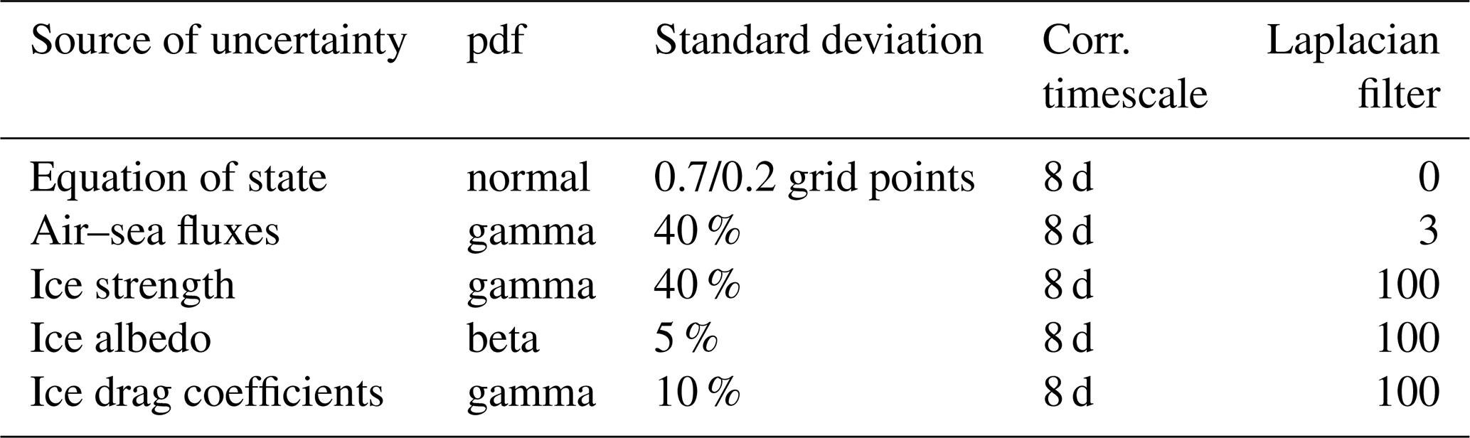
The standard deviation of the equation of state is defined according to longitude and latitude.

Download Print Version | Download XLSX

With this stochastic modelling system, a 70-member ensemble simulation, without assimilation, is performed for the 8-month period between mid-January and mid-September 2011. It will be used to perform the analyses in the present paper. This ensemble simulation yields a probability distribution for the evolution of the system, in particular the ensemble mean, hereafter 〈x_f〉, where 〈⋅〉 indicates an ensemble mean over the members of the ensemble and the background error covariance matrix of the prior ensemble, P_f. Figure 1a and b show, respectively, the ensemble mean (〈x_f〉) and the standard deviation of the prior ensemble. This ensemble is appropriate to illustrate the multiscale analysis in our study. Indeed, as will be shown later, the spread of the ensemble spans a wide range of scales from basin scale to mesoscale. Large scales as well as small structures are well represented, which will allow us to evaluate our separation scale algorithm. Nevertheless, the standard deviation is too small in the regions of strong eddy activity such as the Gulf Stream. This is mainly due to the model configuration (CREG4), which causes an excessive dissipation of the turbulent kinetic energy. Moreover, the variability is too large close to the East Siberian Sea. However, since we are using twin experiments, the simulation does not need to be perfectly realistic to evaluate our approach (providing that the multiscale nature of the problem remains). These characteristics are thus not likely to affect the evaluation of the multiscale algorithm that is performed in this study.

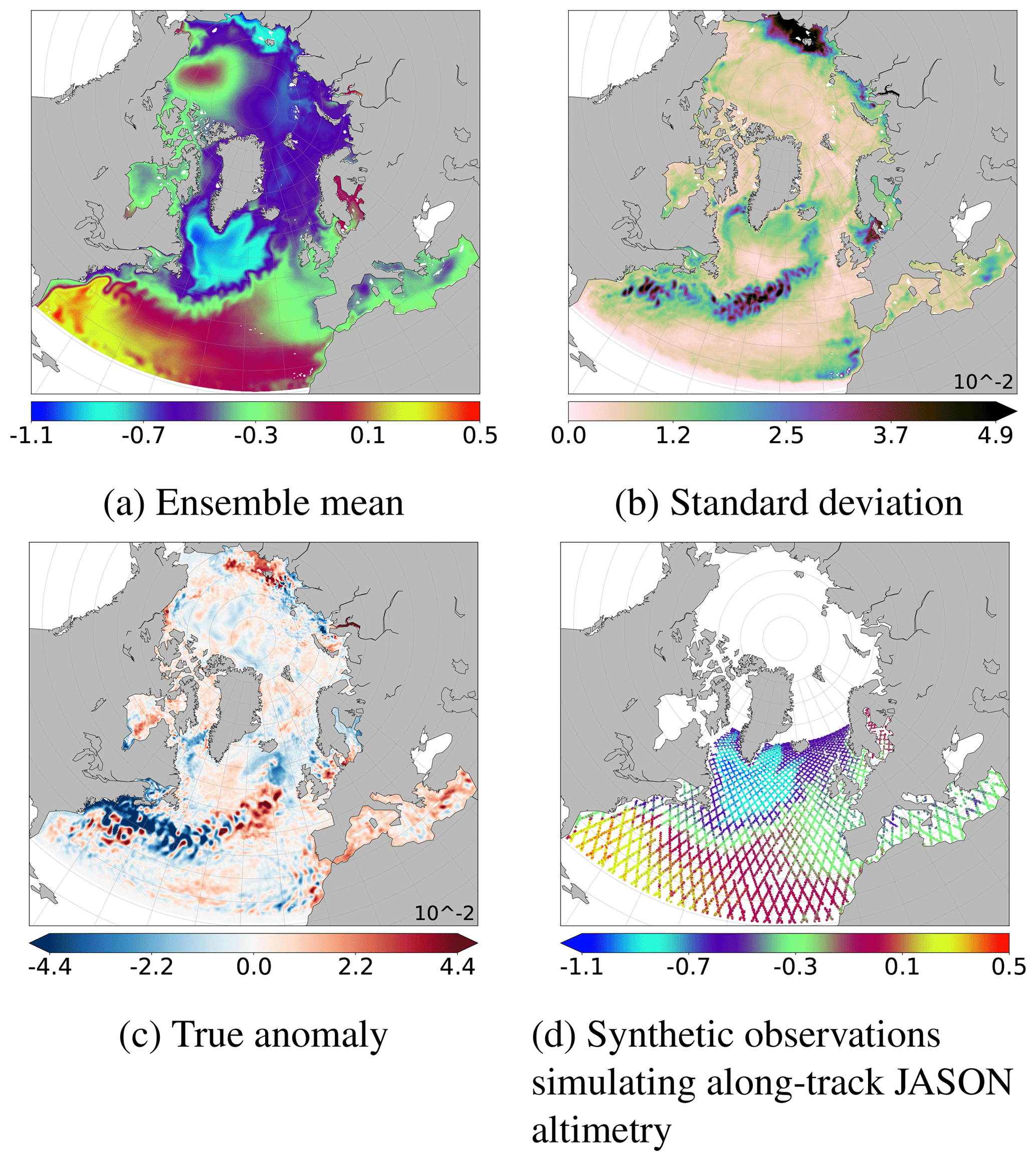
Figure 1SSH (in metres). Ensemble mean (a) and standard deviation (b) of the prior ensemble (N=69 members). The true anomaly (c) is defined as the difference between the true member (computed as an additional independent member of the ensemble) and the ensemble mean (a). Synthetic observations simulating along-track Jason altimetry (d) correspond to the true member along the track of the Jason altimeter plus a noise, following Eq. (1).

Download

2.2 Definition of the twin experiments

The assimilation problem investigated in this study is based on twin experiments with altimetry. In this kind of experiment, the true state is known and synthetic observations are built from this true state. It is generated by the same model to which data assimilation is applied. This method has the advantage that the effectiveness of the different algorithms can be directly evaluated thanks to the known true state. One member of the ensemble simulation is left apart to be used as a reference (the simulated truth) from which the observations will be simulated: x_true. The prior ensemble (indicated thereafter by the subscript f as forecast during an assimilation step) used in the experiments is thus a 69-member ensemble.

In this study, to illustrate the behaviour of the multiscale algorithm, we will concentrate on studying the observational update of the prior ensemble on 30 August 2011. Figure 1c shows the true anomaly: x_true−〈x_f〉. This true anomaly will be used as a reference to evaluate the effectiveness of the different localisation schemes and of the multiscale analysis. Synthetic observations are simulated by adding a simulated observational noise (ϵ: a Gaussian noise with 5 cm standard deviation) to the true state (x_true) with the observation operator (H) along the track of the Jason altimeter:

In this experiment, a 10 d observation window is chosen to have the best coverage provided by Jason. Figure 1d shows the resulting synthetic observation of the sea surface height (SSH). The Jason altimeter does not provide any observation above 66^∘ N latitude. In our example, there is thus no available observation to correct, during the analysis step, the large ensemble variance observed close to the East Siberian Sea (Fig. 1b). This is something that the multiscale approach will have to cope with.

The observational update of the prior ensemble will be performed with a square root algorithm. The analysis scheme used at Mercator Océan is derived from the singular evolutive extended Kalman filter (SEEK) (Pham et al., 1998; Brasseur and Verron, 2006), which is similar to that used in the ensemble transform Kalman filter (ETKF) (Bishop et al., 2001). It can be applied indifferently in the spatial domain as well as in the spectral domain. In the assimilation system, the observational update is usually applied to all model variables. In this paper, however, the effect of the multiscale approach will mainly be evaluated by the update of SSH, which is the observed variable, and by the update of temperature and salinity to illustrate the application of the method to non-observed variables. In the multiscale algorithm developed in this study, nothing will be changed in the core of the square root algorithm: the only novelty is that a spectral transformation is applied before the observational update to allow spectral localisation rather than spatial localisation. A spatial localisation scheme has been already developed and evaluated (Testut et al., 2003; Brankart et al., 2011). For this study, it has been adapted to be used in the spectral domain.

2.3 Ensemble correlation structure

The 69-member ensemble correlation structure (without the true state, which has been left apart) is illustrated in Fig. 2a and b. It has been computed according to two arbitrary reference points: one in the Gulf Stream and the other in the north-east Atlantic Ocean off the coast of Portugal. Ensemble correlation structure shows how the assimilation of an observation at this reference point will influence the other regions during the analysis step. For N=69 members, the correlation coefficient is significant at 95 % if it is larger in absolute value than 0.2367. In both examples, the most important and significant values, i.e. where the observation will have an impact, are mostly confined around the reference point. Some significant correlations are observed further, but their values are lower and not reliable enough to be used during an assimilation step. The usual solution to avoid the spurious effect of non-significant ensemble correlations is to perform a spatial localisation during the analysis step. It consists in completing the correlation structure provided by the ensemble by the assumption that only local correlations are significant and usable (Houtekamer and Mitchell, 1998; Hamill et al., 2001). The long-range correlations are thus assumed to be zero to perform the analysis step.

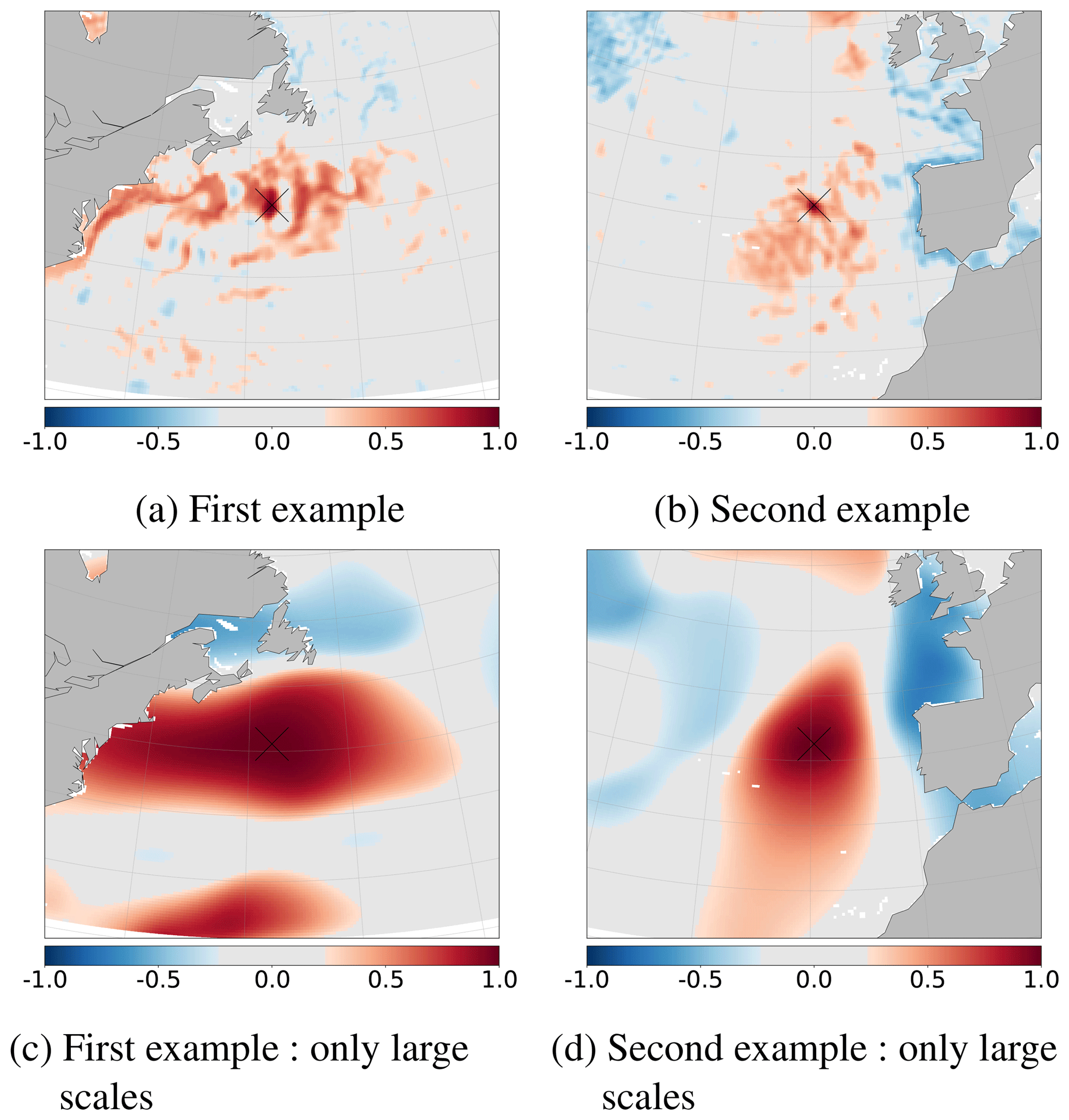
Figure 2Two examples of ensemble correlation for the prior ensemble (SSH), according to two different reference points indicated by black crosses, computed for the full spectrum (a, b) and for the large scales (c, d, $l\in \left[\mathrm{0};l_{\mathrm{c}}\right]$, with l_c=34 following Eqs. 2 and 3, which corresponds to a characteristic scale larger than L≈187 km). Light grey colour corresponds to non-significant values of ensemble correlations for an ensemble of N=69 members (smaller in absolute value than 0.2367 with significance threshold at 95 %).

Download

However, if we look at the same correlation structure (from the same ensemble) for the large-scale component of the signal (characteristic scale larger than L≈187 km), as illustrated in Fig. 2c–d, we see that there are significant correlations over a much larger range. Hence, significant information of the large-scale signal is available even if the size of the ensemble is small. But these are usually masked by the presence of the small-scale signal. In the standard spatial localisation, these large-scale correlations structures are heavily suppressed and thus a part of the large-scale information is not used during the analysis step. The goal is now to find a way to correctly exploit these correlations in the assimilation scheme to better estimate the large-scale signal.

It seems difficult to explicitly control all scales of the system without separating the different spectral components of the signal. In this study, the main idea is to do a spectral transformation of all variables of the system in order to do the analysis in the spectral domain before going back in the spatial domain to do the next steps of the assimilation scheme.

3.1 Forward transformation: projection on the spherical harmonics

The forward transformation step involves transforming each input parameter used for the analysis into the spectral domain, namely each member of the prior ensemble, but also observations and observational errors. A full two-dimensional signal in spherical coordinates, f(θ, ϕ), can be projected on spherical harmonics Y_lm(θ, ϕ) by the following spectral transformation (ST):

where l and m are the degree and order of each spherical harmonics, with l∈ℕ and $\left|m\right|\le l$. In principle, the integral in Eq. (2) extends over the whole sphere Ω. However, in the assimilation system, all fields f(θ, ϕ) that need to be transformed are anomalies with respect to the ensemble mean. In practice, it is thus possible to extend f(θ, ϕ) with zeroes outside the available domain ($f\left(\mathit{\theta },\mathit{\varphi }\right)=\mathrm{0}$ on continents and outside the model domain) in order to compute the integral over the whole sphere. For a multivariate three-dimensional variable, this transformation can be applied to each vertical level of each model variable.

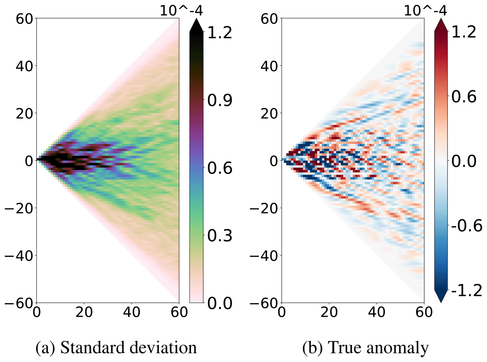
This spectral transformation provides a new point of view on the ensemble because it separates scales. Each degree l of the spherical harmonic indeed corresponds to a wavelength of a spherical harmonic $\mathit{\lambda }=\frac{\mathrm{2}\mathit{\pi }{R}_c}{l}$, with R_c the Earth's radius, and thus to a characteristic scale $L=\frac{\mathit{\lambda }}{\mathrm{2}\mathit{\pi }}$. This reversible spectral transformation preserves the information for each degree l. The coefficients f_lm of the spherical harmonics decomposition can be computed for each degree l up to a selected degree l=l_max. This transformed field contains the same information, until l_max, as shown in the spatial domain in Fig. 1. The coefficients f_lm of each member of the prior ensemble have been computed for the SSH until the degree l_max=60, which corresponds to a wavelength λ≈667 km and a characteristic length L≈106 km. Figure 3a shows the standard deviation of this prior ensemble in the spectral domain. Figure 3b shows the result of the spectral transformation applied to the true SSH anomaly, i.e. the coefficients f_lm of the true SSH anomaly. Similar patterns have been observed by Wunsch and Stammer (1995) from early altimetric observations. Most of the variability is concentrated at large scales (small l). The variance becomes weak for meridional structures, i.e. for $\mid m\mid \to l$.

Figure 3Standard deviation (a) of the prior ensemble and true anomaly (b) in the spectral domain (SSH), according to the degrees $l\in [\mathrm{0},\mathrm{60}]$ in the abscissa and m in the ordinate; see Eq. (2), which corresponds to a characteristic scale larger than L≈106 km.

Download

3.2 Backward transformation: scale separation

From the spectrum f_lm, the field $f_{l_{\min }}^{l_{\max }}\left(\mathit{\theta },\mathit{\varphi }\right)$ can be reconstructed using the inverse transformation:

This inversion can be constrained to specific scales by choosing the values of l_min and l_max. The full field can be reconstructed since $f\left(\mathit{\theta },\mathit{\varphi }\right)=f_{\mathrm{0}}^{\mathrm{\infty }}\left(\mathit{\theta },\mathit{\varphi }\right)$. This is how the method separates scales.

Any spectral band can thus be extracted by choosing the range [l_min; l_max] appropriately. Figure 4 shows the result of the extraction of the large scales applied to each member of the ensemble and to the true anomaly to keep only the large scales. In this case, l_min=0 and l_max=34, which corresponds to a wavelength λ≈1177 km and a characteristic scale L≈187 km. Small-scale structures have been properly removed and only large-scale structures remain visible on the figure.

Figure 4Ensemble mean (a), standard deviation (b) of the prior ensemble and true anomaly (c) for the SSH (in metres), after extraction of the large scales ($l\in \left[\mathrm{0};l_{\mathrm{c}}\right]$, with l_c=34, which corresponds to a characteristic scale larger than L≈187 km; see Eq. 3).

Download

The use of spherical harmonics is not the most natural way to separate scales for fields that do not extend over the whole sphere. In principle, it would, for instance, be better to use the eigenfunctions of the Laplacian operator defined for the model domain. They would account for the land barriers and would display a better relation to the system dynamics. However, they would also be much more expensive to compute than the spherical harmonics and would need to be stored and then loaded each time they are needed to separate scales. This is why we preferred using spherical harmonics in this study: they make the method numerically efficient and they are sufficient to obtain a relevant spectral decomposition of the input signal.

3.3 Transformation of the observations

In theory, transformation of observations is not needed to separate scales in the assimilation system. It should be sufficient to introduce the scale separation operator in the observation operator of the existing algorithm. However, for practical reasons, the algorithm that we are proposing requires a preprocessing of the observations to separate scales. This is done to keep the algorithm easy to implement in an existing system: nothing new needs to be implemented except the scale separation operator and to keep the resulting algorithm efficient enough to be applicable to a large-size assimilation system.

In this section, we show how this transformation of observations can be performed by regression of the observations on the spherical harmonics (see Sect. 3.3.1) and how the statistics of the observational errors can be transformed accordingly (see Sect. 3.3.2).

3.4 Transformed correlation structure

We need to study the main dependencies and correlations between the different spectral components of the ocean fields in order to determine whether and how the scale separation could be used in the data assimilation scheme. Figure 5 shows two examples of ensemble correlation maps between spectral amplitudes. It is comparable to Fig. 2 but in the spectral domain (amplitudes f_lm of Eq. 2). Ensemble correlation structure is computed according to reference points in the spectral domain and indicated by crosses in Fig. 5. It shows how the assimilation of the signal of an observation at these reference points will impact the other scales during the spectral analysis step. Similarly to Fig. 2, the significant and maximum area is confined near the reference points. Most correlations between very different scales are weak and might thus be neglected by data assimilation. This is the basic property allowing to introduce scale separation in the data assimilation scheme with a reasonable cost. However, it is true that there are also significant correlations for remote scales, and that neglecting these correlations corresponds to losing potentially useful information. This is however similar to what happens with spatial localisation: in Fig. 2, there also exists significant correlations far from the reference location. The question is then which correlations is it better to neglect to preserve the meaningful structures contained in the ensemble. This is the question that we will try to elucidate with our example application.

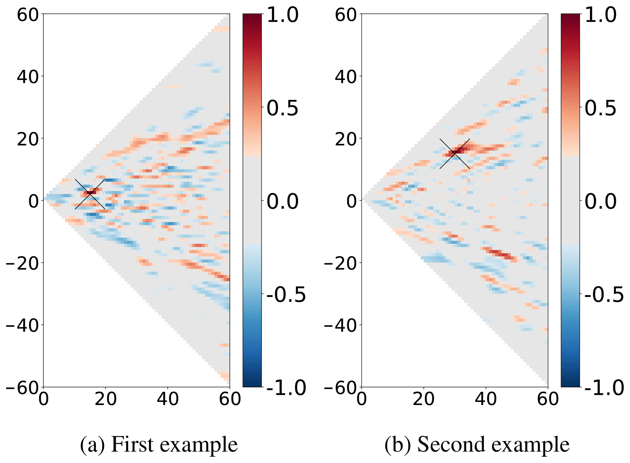
Figure 5Two examples of ensemble correlation for the prior ensemble (SSH) in the spectral domain, according to the degrees $l\in [\mathrm{0},\mathrm{60}]$ in the abscissa and m in the ordinate; see Eq. (2). The two different reference points are indicated by black crosses. Light grey colour corresponds to non-significant values of ensemble correlations for an ensemble of N=69 members (smaller in absolute value than 0.2367 with significance threshold at 95 %).

Download

To exploit this property of weak correlations between very different scales, a spectral analysis thus also requires to be localised, at least for the large scales in our study. The method of spectral localisation is the same as that usually used in the spatial domain. For the same reasons, each localisation window will contain a number of degrees of freedom sufficiently low to be controlled with an ensemble of moderate size.

4.1 Multiscale observational update algorithm

We propose an algorithm for the multiscale analysis based on a combination of a spectral analysis with spectral localisation for the large scales (described by Eq. 7) and a spatial analysis with spatial localisation for the residual scales (described by Eq. 6). The large scales are defined by the critical scale l_c. The full algorithm is explained by Eqs. (8) to (12). For this new method, we need to combine an algorithm to perform the observational update (OU) of the ensemble with the forward (ST) and backward (ST⁻¹) spectral transformations previously defined by Eqs. (2) and (3). Any observational update algorithm can be chosen provided that it allows localisation, for instance, the SEEK observational update (Brasseur and Verron, 2006) or the ETKF observational update (Bishop et al., 2001). This localisation will be applied in our case in the spectral domain (OU_spectral) or in the spatial domain (OU_spatial) depending on the context.

4.2 Comparison of localisation schemes

The relevance of implementing a multiscale analysis rather than the usual spatial localisation is only validated if spectral localisation better retrieves large-scale patterns of the signal than spatial localisation. To verify the validity of this assumption, we perform two different analyses in the context of the twin experiments described in Sect. 2.2. The first analysis is carried out with a spatial localisation only following Eq. (6), hereinafter called spatial localisation, whereas the second analysis uses a spectral localisation only following Eq. (7), hereinafter called spectral localisation. Spatial and spectral localisation radius have been optimised to obtain the best results in both experiments. The spatial localisation radius corresponds to a wavelength of spherical harmonic about 139 km at the Equator, while that of spectral localisation is a rectangle of 3 in ordinate l number and 1 in m number. They have been deduced from the correlation ensemble (see, for instance, Fig. 2a and b for spatial localisation, and Fig. 5a and b for spectral localisation). The localisation radius is chosen small enough to avoid non-significant correlations. In order to evaluate these localisation algorithms, they are compared for the large scales. As justified later in Sect. 4.3, we choose to define large scales as the range of scales $l\in \left[\mathrm{0};\mathrm{34}\right]$.

Each scale of spatial and spectral analysis increments has to be as close as possible to the corresponding scale of the true anomaly. The large-scale part of this spatial analysis increment ($\mathit{\delta }{\mathit{x}}_a^i$ of Eq. 6) can be directly compared to the spectral analysis increment obtained from the large scale of the prior ensemble ($\mathit{\delta }{\mathit{x}}_a^{i,\mathrm{LS}}$ of Eq. 7). It can be extracted, following Eqs. (2) and (3), to obtain the corresponding large scales of the spatial analysis increment:

Simultaneously, the obtained spectral analysis increment (Eq. 7) is back into the spatial domain (applying ST⁻¹, following Eq. 3) to be directly comparable to the large scales of the spatial analysis increment (Eq. 13). Figure 6a and b show, respectively, the large scale of the mean ensemble of analysis increments obtained, respectively, with spatial localisation or spectral localisation (see Sect. 4.1.1). Hence, they have to be as similar as possible to the large-scale part of the true anomaly shown in Fig. 4c.

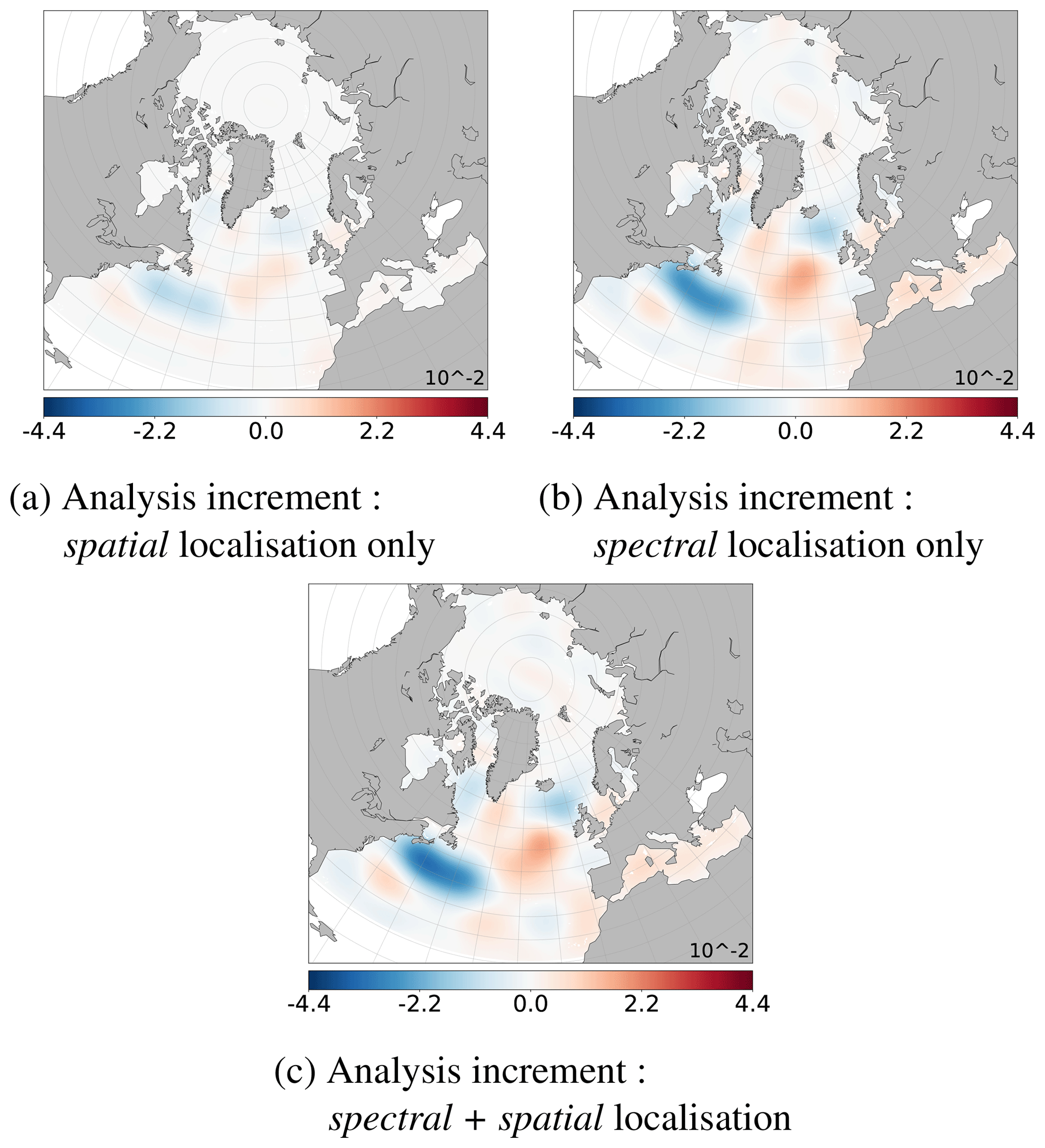
Figure 6Ensemble mean of large-scale part of the analysis increments (SSH in metres), with $l\in \left[\mathrm{0},l_{\mathrm{c}}\right]$, l_c=34: (a) obtained after spatial localisation only and then filtered; see Eqs. (6) and (3); (b) obtained after spectral localisation following Eq. (7); (c) obtained after multiscale analysis (spectral + spatial localisation; see Sect. 4.1.2) (to be compared to the large-scale true anomaly, Fig. 4c).

Download

Spectral localisation recovers large scales much better than spatial localisation; see Fig. 6 vs. Fig. 4c. In all cases, the analysis increment is significant only where Jason data are available (see Fig. 1d). The analysis and the type of localisation thus have no significant impact on the north of the model domain. This result reinforces the idea of a multiscale analysis with spectral localisation for the large scale. It is now necessary to determine the critical scale, l_c, from which the spatial localisation will be preferred.

4.3 Determining the critical scale

On average, spectral localisation only gives better results than spatial localisation for the large scales, but we need to check that this affirmation remains valid at each scale or that there exists a critical scale, l_c, from which this tendency is no longer true. To determine l_c, a classic score is computed for the spatial localisation and the spectral localisation. It shows the improvement of the RMSE after/before the analysis by averaging sums over the whole model domain:

where $\stackrel{\mathrm{‾}}{\cdot }$ is the mean over the domain. Each member of this equation is then computed for all specific degree l, following Eqs. (2) and (3) with $l_{\min }=l_{\max }=l$. During an analysis step, the RMSE of the observed variable will be reduced. The ratio thus allows to evaluate the accuracy of the analysis for each scale. Figure 7 shows this score for each degree l until 100 for the spatial analysis only and until 60 for the spectral analysis only.

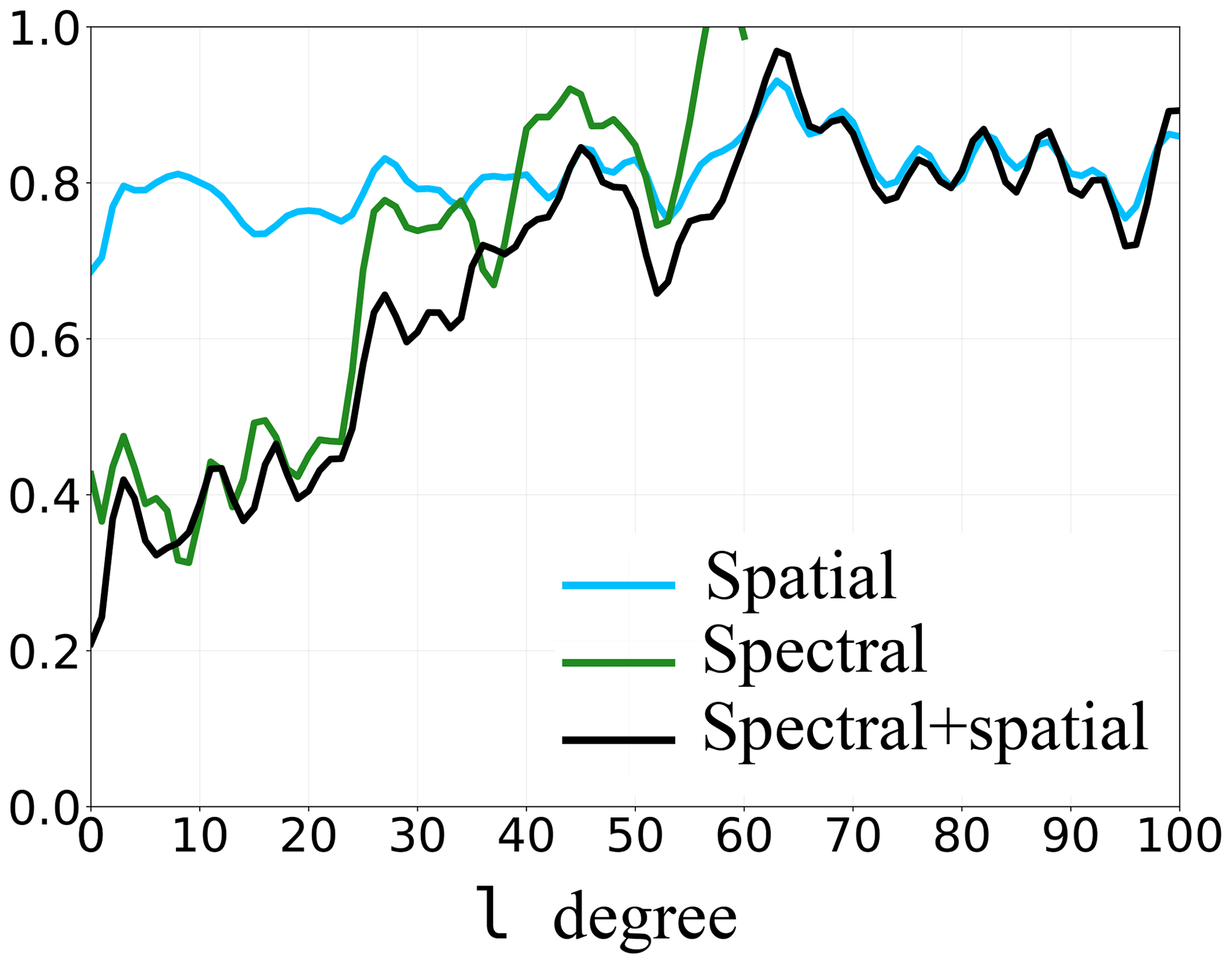
Figure 7Reduction of spatial RMSE for each degree for the SSH, computed using Eq. (14). The blue curve (spatial) refers to the spatially updated ensemble, the green curve (spectral) to the spectrally updated ensemble and the black curve (spectral + spatial) to the multiscale updated ensemble.

Download

This gives a new point of view to evaluate the results of an analysis, giving the efficiency of the spatial or spectral analysis at each scale and no longer only for the full field. Spatial localisation deals with all scales at the same time. The score is almost the same at each scale: around 0.8. In contrast, this score of the spectral localisation is very sensitive to the scale. It is almost up to 2 times smaller than the one of the spatial localisation for the large scales. It increases with the degree until it becomes similar and exceeds the spatial localisation score. The spectral observational error used for the spectral localisation has not been computed exactly from l≈50. This led to important values close to l=60, which impact the score shown in Fig. 7. However, if observational error has been computed exactly until larger degrees, the trend would follow a similar pattern.

Until around l≈34, spectral localisation further reduces the spatial RMSE more than spatial localisation, which is consistent with the study of analysis increments in Fig. 6, while, for larger degrees l, this trend tends to reverse. The critical value, l_c, does not need to be very precise for the multiscale analysis. Indeed, the scores of spatial and spectral localisations are close on a range of degrees (here around 30 and 50, for instance). A variation of a few degrees on l_c will not have any major impact on the final results of the multiscale analysis. In this twin experiment and for all these reasons, the critical scale l_c is now fixed to l_c=34.

5.1 Error reduction at each wavelength

On average, the updated ensemble produced with the multiscale analysis should better approach the true state than those obtained with the spatial localisation only. To evaluate the efficiency of the multiscale analysis, the error has been computed in two ways: at each scale in the spectral domain, following Eq. (14), and in the spatial domain for the full spectrum, with a comparison of the analysis increments and the true state.

5.1.2 Spatial global point of view: analysis increment

The analysis increments obtained with spatial localisation (Fig. 8a) or with multiscale analysis (spectral + spatial localisation; Fig. 8b) can be directly compared to the full spectrum of the true anomaly shown in Fig. 1c. The multiscale analysis allows to recover a part of the large-scale pattern unlike the spatial localisation. It keeps advantages of the spatial localisation for the residual scales.

Figure 8Same as Fig. 6a and c but keeping the full spectrum (no extraction of the large scales): (a) obtained after spatial localisation only, following Eq. (6); (b) obtained after multiscale analysis (spectral + spatial localisation) following Sect. 4.1.2 (to be compared with Fig. 1c).

Download

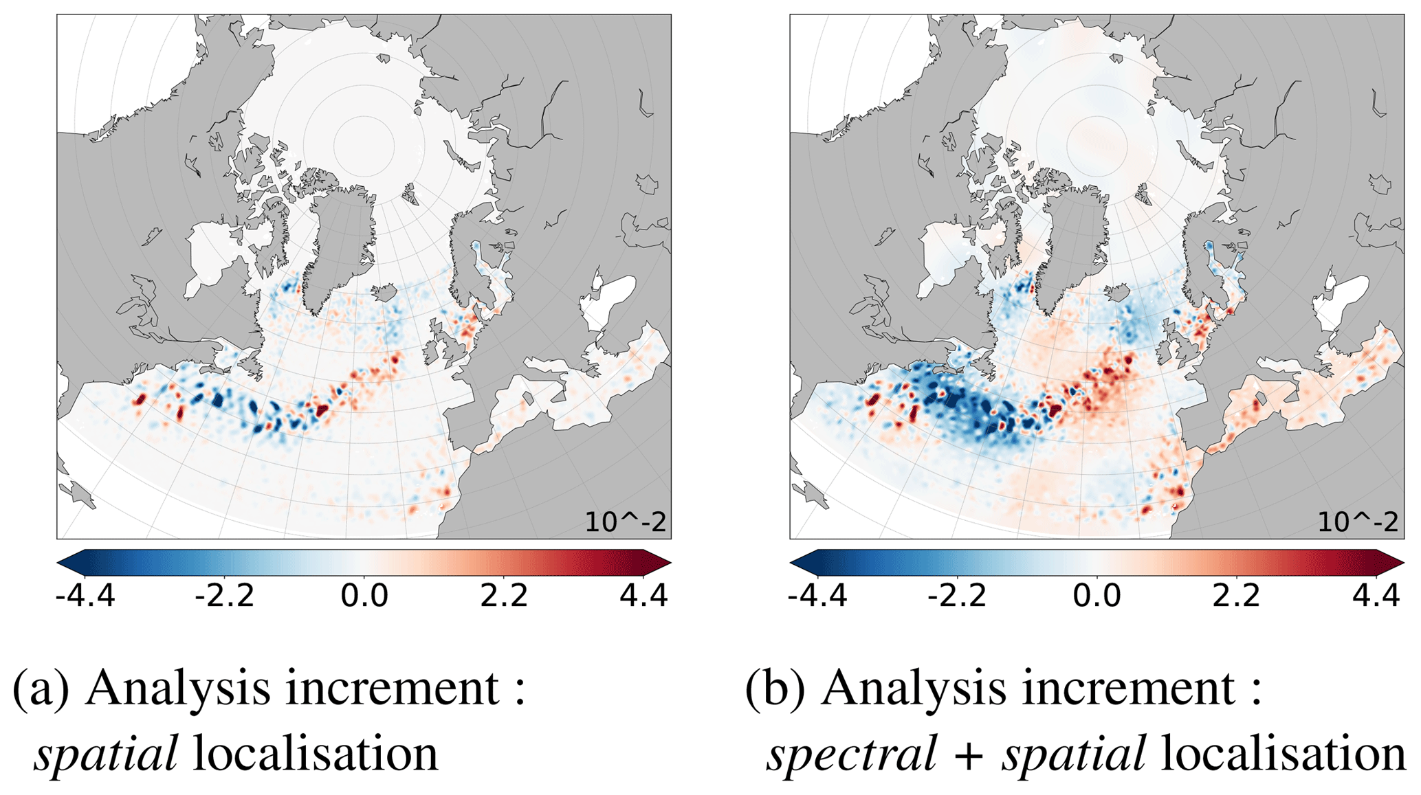
These analysis increments can be evaluated at each scale. Figures 6a and c show the large scales ($l\in \left[\mathrm{0};\mathrm{34}\right]$) of these analysis increments, respectively, for spatial localisation or multiscale analysis. They have been obtained from their respective full fields (Fig. 8a and b) following Eqs. (2) and (3). Small structures have been well removed from the full spectrum. They have to be as close as possible to the large scales of the true anomaly shown Fig. 4c, which have been extracted from its full field shown in Fig. 1c. Multiscale analysis and spectral localisation give similar results for the large scales and are better than the spatial localisation. This is consistent with observed reduction of spatial RMSE at each large scale, shown in Fig. 7.

5.2 Reliability of the updated ensemble

The updated ensemble should be reliable in the spatial domain but also in the spectral domain. This involves checking the coherence between the assumed probabilities and the observed statistics when the ensemble is compared to the verification data (the true state in our twin experiment, or observation in a real system). To check ensemble reliability, ranks are traditionally computed in the spatial domain and summarised in a rank histogram. They show the distribution of observations with respect to the ensemble (Anderson, 1996; Talagrand et al., 1997). In our context of twin experiments, the prior ensemble is reliable by construction. Indeed, the true state originates from the same ensemble simulation as the other members. The reliability of the updated ensemble will be evaluated by comparing the rank histogram of the updated ensemble with the rank histogram of the prior ensemble. Hence, a flat rank histogram indicates a reliable ensemble, whereas a U-shaped rank histogram indicates a lack of spread in the ensemble: the uncertainty is underestimated (Anderson, 1996; Hamill, 2001). Alternatively, we propose a new point of view of these ranks, computing them in the spectral domain. The interpretation of these new ranks has to corroborate the conclusions obtained in the spatial domain.

5.2.1 Spatial rank histograms

Rank histograms have been computed, with respect to the true state, from spatial maps limited to the Jason domain for the prior ensemble, the spatially updated ensemble and the multiscale updated ensemble. Figure 9b shows the rank histograms for the large scales ($l\in \left[\mathrm{0};l_{\mathrm{c}}\right]$) for the same ensembles but also for the spectrally updated ensemble presented in the previous section.

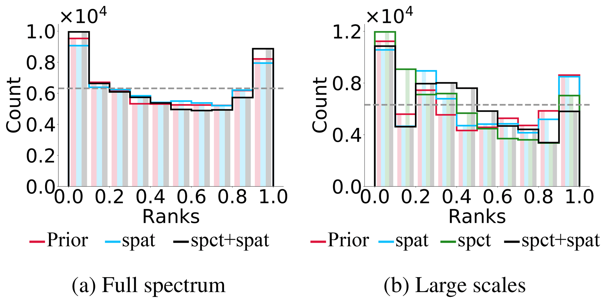
Figure 9Spatial rank histogram on the Jason domain for the SSH. “Prior” (in red), “spat” (in blue), “spct” (in green) and “spct + spat” (in black) correspond, respectively, to the prior ensemble, spatially updated ensemble, spectrally updated ensemble and the multiscale updated ensemble. (a) Full spectrum; (b) after extraction of the large scales: $l\in \left[\mathrm{0};l_{\mathrm{c}}\right]$, with l_c=34.

Download

Rank histograms show that all these updated ensembles can be considered as reliable as the prior ensemble, both for the full spectrum and for the large scales. Indeed, the prior ensemble looks somewhat underdispersed but can be considered reliable because the true member originates from the ensemble itself. The rank histograms of the updated ensembles are of the same order of magnitude as that of the prior ensemble. Thus, the small underdispersion of the prior ensemble (which can only result from the limited size of the sample) has not increased during the analysis step. These consistent rank histograms confirm that the observational error has been properly evaluated.

5.2.2 A new point of view: ranks map in the spectral domain

Reliability of all updated ensemble (spatial localisation only and multiscale analysis) is now tested for degrees $l\in \left[\mathrm{0};\mathrm{60}\right]$ by calculating ranks in the spectral domain with respect to the true state. Ranks are computed following the same procedure as in the spatial domain but the members and the true state are previously transformed into the spectral domain following Eq. (2). Figure 10 shows the maps of ranks in the spectral domain for the prior ensemble, the spatially updated ensemble and the multiscale updated ensemble. The maps of ranks for the spectrally updated ensemble are not shown due to similar results to the multiscale updated ensemble. This new point of view allows to diagnose the behaviour of the system for each scale.

Figure 10Maps of ranks in the spectral domain for the SSH, according to the degrees $l\in [\mathrm{0},\mathrm{60}]$ in the abscissa and m in the ordinate; see Eq. (2). (a) Prior ensemble; (b, c) updated ensembles, respectively, obtained after spatial localisation only (see Eq. 6) or after the multiscale analysis (spectral + spatial localisation; see Sect. 4.1.2).

Download

Ranks maps in the spectral domain provide additional indication that all algorithms provide reliable updated ensembles. Observational error has been consistently evaluated. The ranks are computed for each spectral coordinate (l, m) and have been normalised by the total number of data points to have numbers between 0 and 1. For a perfectly reliable ensemble, ranks would be evenly and randomly distributed over the entire spectral domain. For our study, when degrees tend toward l=m, which corresponds to meridional signal, ranks are not all represented even for the prior ensemble. However, these spectral regions correspond to extremely weak standard deviation of the ensemble in the spectral domain (see Fig. 3a): there is no meridional signal in the prior ensemble. They do not have an important impact on the spatial field. For the other degrees, ranks show that the prior ensemble is reliable. The spatially updated ensemble and the multiscale updated ensemble also remain reliable even if the latter seems to be somewhat less dispersed.

5.3 Resolution of the updated ensemble

The spread, or variance, of the prior and the updated ensemble (with N=69 members) has been computed to check the resolution of the updated ensemble. For instance, for the prior ensemble, x_f,

The reliability of the ensemble has been checked previously with the rank histograms. Then, the smaller the spread after the analysis, the better the analysis. Figures 11 and 12 show the spread of the prior ensemble, the updated ensemble after spatial localisation and the updated ensemble after a multiscale analysis (spectral + spatial localisation), respectively, for the full spectrum and after extraction of the large scales ($l\in \left[\mathrm{0},l_{\mathrm{c}}\right]$, with l_c=34).

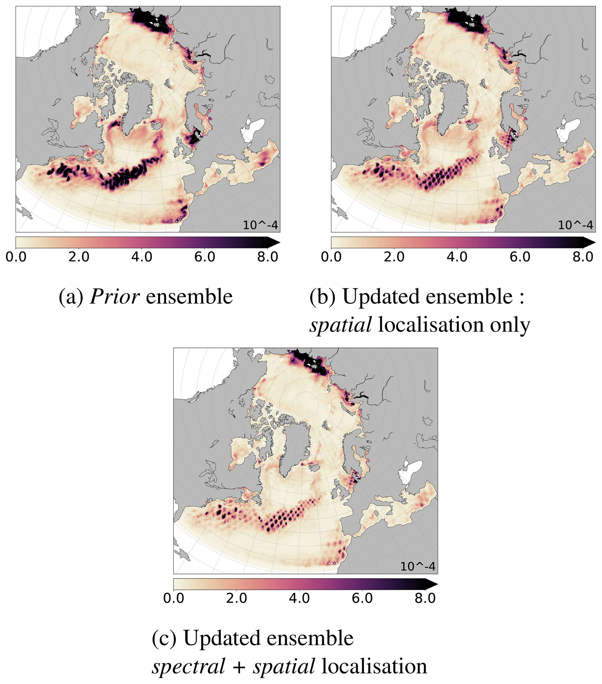
Figure 11Ensemble spread of the prior (a), the updated ensembles obtained with (a) the spatial localisation only or with (c) the multiscale analysis (spectral + spatial localisation), according to Eq. (15) (full spectrum) for the SSH.

Download

The multiscale analysis allows to decrease the ensemble spread more than the spatial localisation. The spread is much more reduced along Jason tracks; see Fig. 11c. This decrease is especially important for the large scales; see Fig. 12c. For the large scales, the spread of the updated ensemble by spectral localisation is not shown due to similar results to those of multiscale analysis. Thus, knowing that all these ensembles are reliable, the more efficient algorithm is the multiscale analysis because it has further reduced the spread of the ensemble and is the closest to the true state.

Figure 12Same as Fig. 11 but after extraction of the large scales ($l\in \left[\mathrm{0};l_{\mathrm{c}}\right]$, with l_c=34; see Eqs. 2 and 3).

Download

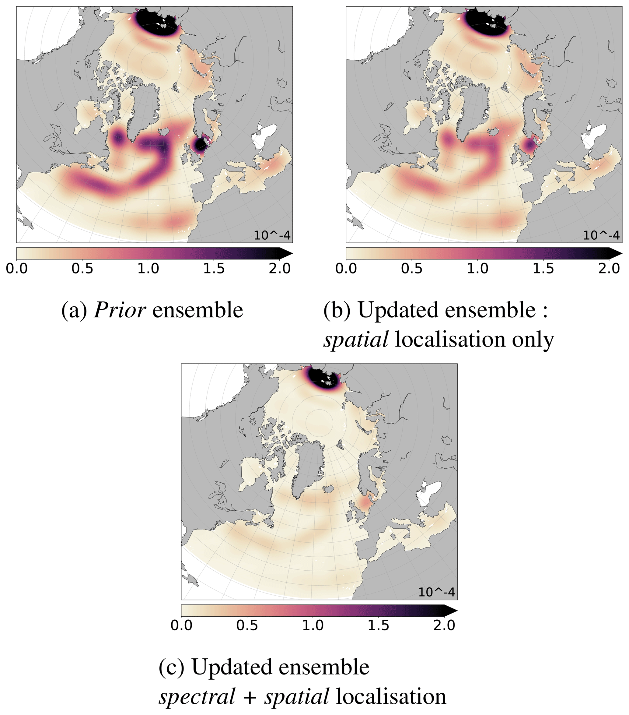
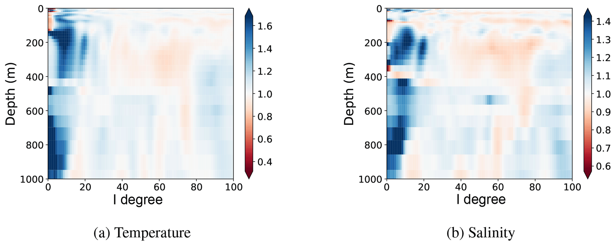
Figure 13Improvement obtained by the multiscale analysis for temperature (a) and salinity (b). This improvement is measured by comparison to spatial localisation only using the ratio in Eq. (16). Blue (respectively red) colour corresponds to a better (respectively worse) correction of the error using the multiscale analysis as compared to spatial localisation only.

Download

5.4 Multivariate analysis

Multivariate analysis consists in extending the observational update to non-observed variables, like temperature and salinity, in the state vector during the analysis. The experimental setup remains the same. The aim is to evaluate the impact of the multiscale analysis on these non-observed variables and to check that it does not introduce more error than the spatial localisation. These errors could increase during the next forecast and cause some unrealistic values. For this purpose, we compute the score defined by Eq. (14) for each degree for the spatial localisation (spat) and for the multiscale analysis (spct+spat). Then, we compute, for each level and each degree, the ratio of these scores, following Eq. (16).

Figure 13 shows these results for the temperature and salinity. Each depth in this figure thus corresponds to the ratio of the blue and black curves of Fig. 7, no longer for the SSH but for the temperature or salinity instead of SSH.

On average, below and around the critical degree l_c=34, the multiscale analysis further reduces the error as compared to the spatial localisation only. In a few cases, at basin scales, multiscale analysis appears to produce poorer results than spatial localisation. However, this effect is small as compared to the improvement made at the other depths and large scales. For smaller scales, these two analyses give similar results. It is consistent with the fact that a similar spatial localisation is done for the both analyses and with the results obtained for SSH (see Fig. 7).