2.1 The Hybrid Coordinate Ocean Model

The Hybrid Coordinate Ocean Model (HYCOM) is a primitive equation ocean model that was developed from the Miami Isopycnic Coordinate Ocean Model (MICOM) (Smith et al., 1990). HYCOM combines the optimal features of isopycnic coordinates and fixed-grid ocean circulation models into one framework (Bleck, 2002) and uses the hybrid layers to change the vertical coordinates depending on the stratification of the water column. The model makes a dynamically smooth transition between the vertical coordinate types via the continuity equation using the hybrid coordinate generator (Chassignet et al., 2007). Well-mixed surface layers use z-level coordinates, ρ coordinates are utilized between the surface and bottom layers in a well-stratified ocean, and the bottom layers apply σ coordinates following bottom topography. Adjusting the vertical spacing between the hybrid coordinate layers in HYCOM simplifies the numerical implementation of several physical processes without affecting the efficient vertical resolution, and thus combines the advantages of the different coordinate types in optimally simulating coastal and open-ocean circulation features (Chassignet et al., 2007).

This study used output from a one-way nested 1∕10^∘ model of the greater Agulhas Current system (AGULHAS) (Backeberg et al., 2008, 2009, 2014). The regional nested model, AGULHAS, received boundary conditions from the basin-scale model of the Indian Ocean and Southern Ocean (INDIA) (George et al., 2010) every 6 h. The boundary conditions were relaxed towards the outer model over a 20 grid cell sponge layer. The nested model covered the region from the Mozambique Channel to the Agulhas retroflection region and the Agulhas return current, geographically extending from approximately 0 to 60^∘ E and from 10 to 50^∘ S, with a horizontal resolution of ∼10 km that adequately resolved mesoscale dynamics to the order of the first baroclinic Rossby radius estimated to be about 30 km (Chelton et al., 1998). AGULHAS has 30 hybrid layers and targeted densities ranging from 23.6 to 27.6 kg m⁻³.

AGULHAS was initialized from a balanced field of the parent model interpolated to the high-resolution grid and ran from 1980 to 2014 using interannual forcing from ERA40 (Uppala et al., 2005) and ERA-Interim (Dee et al., 2011). Version 2.2 of the HYCOM source code has been used in this model and, together with the second-order advection scheme, provides an adequate representation of the Agulhas Current (Backeberg et al., 2014). However, limitations of the free-running model include high levels of sea surface height (SSH) variability south of Madagascar and offshore of the Agulhas Current, suggesting that eddy trajectories may be too regular in the model (Backeberg et al., 2014). The data available for this study were a weekly output of the regional HYCOM simulation of the Agulhas region from 1980 to 2014.

2.2 The Agulhas Current Time-series Experiment

The ACT was established to obtain a multi-decadal proxy of Agulhas Current transport using satellite altimeter data. The first phase of the experiment was the in situ phase where the ACT mooring array was deployed in the Agulhas Current, near 34^∘ S, for a period of 3 years from 2010 to 2013 (Beal et al., 2015) (Fig. 1). From the data collected, Beal et al. (2015) provided two volume transport estimates: (1) a box or boundary layer transport (T_box) and (2) a western boundary jet transport (T_jet). T_box is the net transport within a fixed distance from the coast, while T_jet is a stream-dependent transport that is calculated by changing the boundaries of integration at each time step depending on the strength and cross-sectional area of the southwestward jet. The western boundary jet transport algorithm was developed to specifically exclude the northeastward transport during meander events, occurring inshore of the meander (Beal et al., 2015). During the second phase of the ACT, Beal and Elipot (2016) built a 22-year transport proxy by regressing the 3 years of in situ transport measurements (obtained from phase 1 against along-track satellite altimeter data spanning the years 1993–2015.

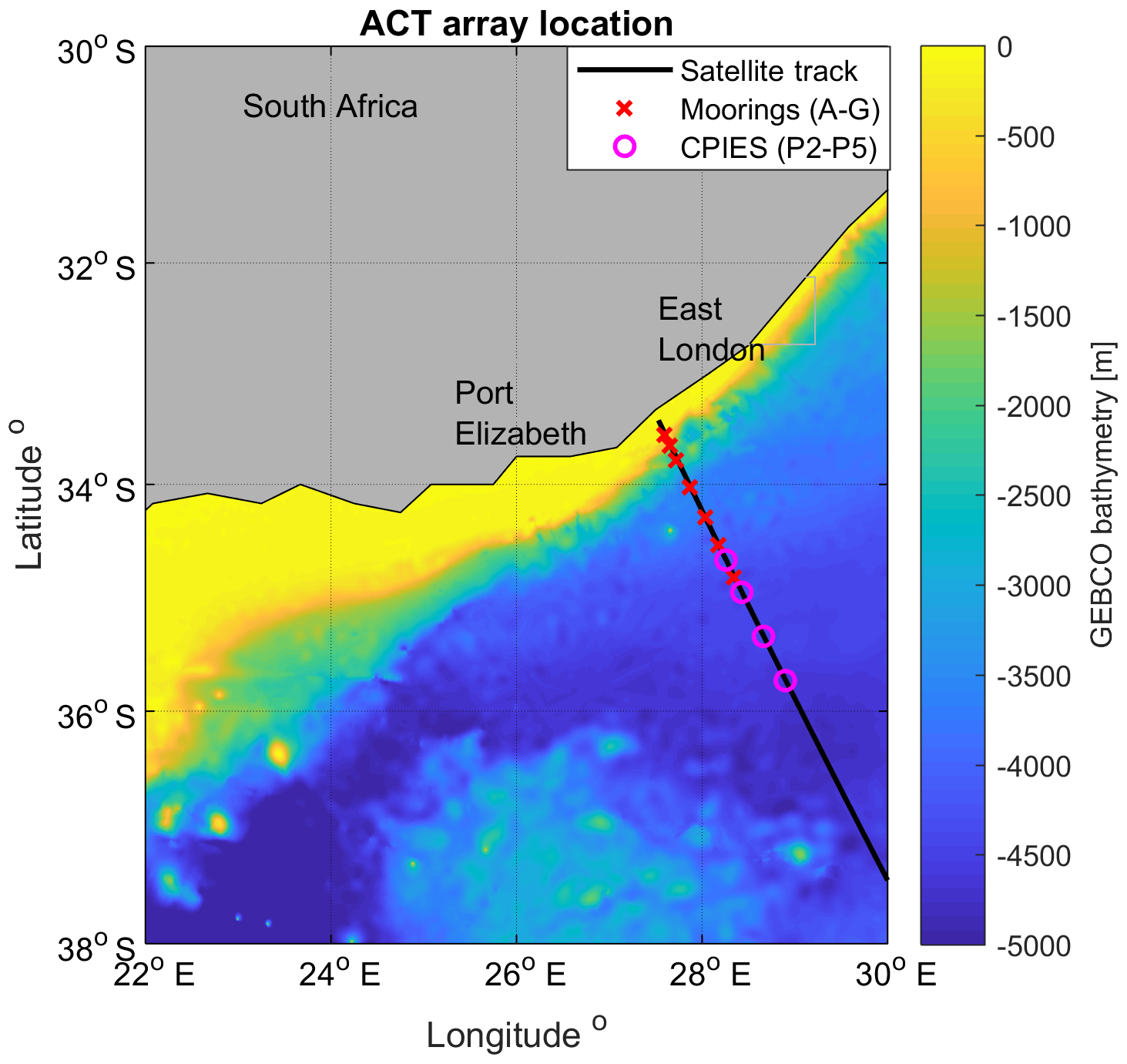
Figure 1Geographical location of the ACT array with the mooring (red crosses) and CPIES (magenta circles) stations relative to the T/P, Jason-1,2,3 satellite track #96 (black line). Colour shading illustrates bathymetry (metres) obtained from GEBCO (General Bathymetric Chart of the Oceans).

Download

2.3 Development of the Agulhas transport proxy

Previous analyses have shown that the vertical structure of the Agulhas Current is barotropic (Elipot and Beal, 2015), implying that the relationship between surface geostrophic velocity and full depth transport should be strong, despite the presence of the Agulhas Undercurrent (Beal and Elipot, 2016) (Fig. 2). Access to the data from the ACT allowed us to validate the velocity cross section in HYCOM (Fig. 2). Beal et al. (2015) defined the Agulhas Current to be 219 km wide and 3000 m deep on average, as is reflected in the vertical section of the in situ ACT observations (Fig. 2a). In HYCOM the current is wider, weaker, and further offshore than the observed current, on average the current is 254 km wide and extends deeper down to ∼3500 m, particularly inshore with a less pronounced undercurrent (Fig. 2b).

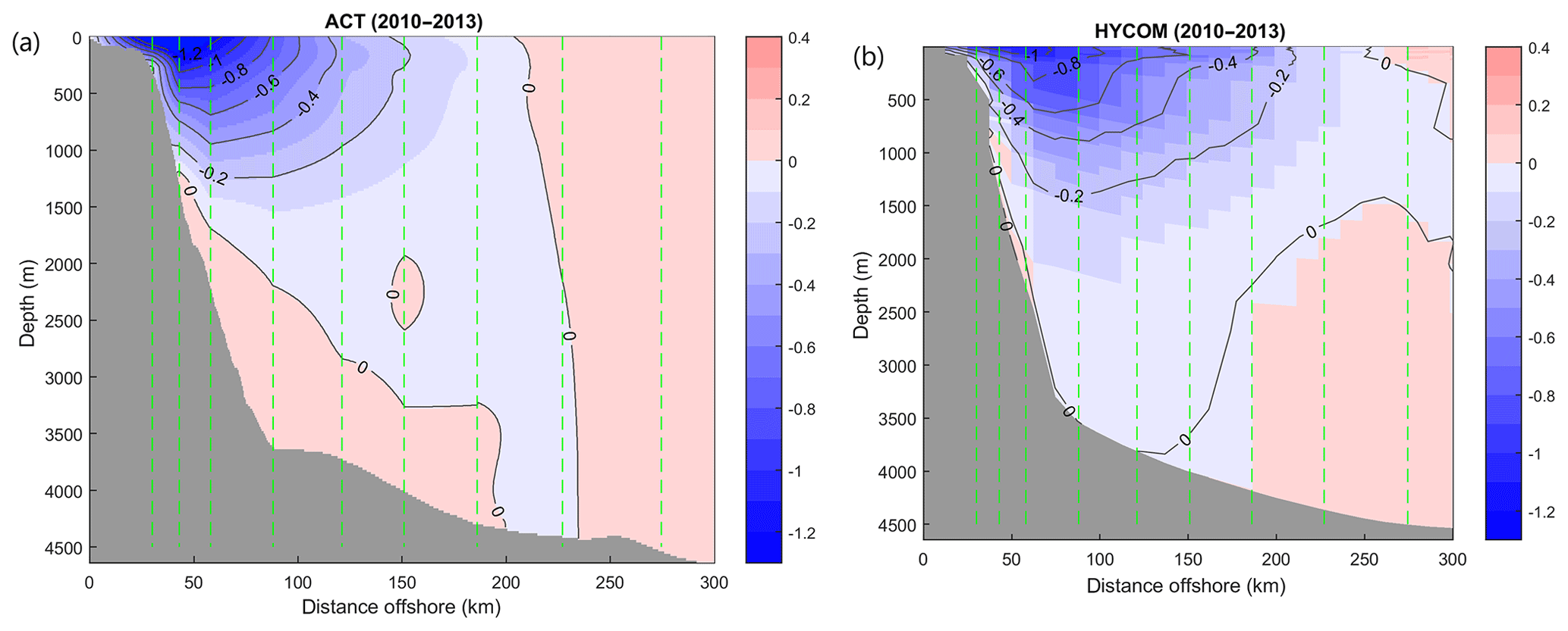
Figure 2Time mean cross section of the velocity structure of the Agulhas Current across the ACT array (m s⁻¹) during the in situ ACT period (2010–2013) from (a) the ACT observations and (b) the HYCOM. Blue shading represents the negative, southwest current flow and pink shading represents the positive, northeast current flow. Contours are every 0.2 m s⁻¹. Dashed green vertical lines represent the nine locations of the mooring and CPIES pairs, the first line representing mooring A and CPIES pair P4P5 furthest offshore.

Download

The transport proxy created by Beal and Elipot (2016) was initially developed by finding a linear relationship between transport and sea surface slope across the entire length of the ACT array, a common method used in previous studies (Imawaki et al., 2001; van Sebille et al., 2010; Sprintall and Revelard, 2014; Yan and Sun, 2015). However, this method led to uncertainty in the linear regression due to the strong, co-varying sea surface height across the current. The preferred method was therefore to build nine individual linear regression models, one for each mooring position and CPIES pairs along the ACT array, which locally related transport to sea surface slope (Beal and Elipot, 2016). It is important to note that the regression models assumed a constant, linear relationship between sea surface slope and transport over the 3-year in situ period. The transport variable in the regression models was defined as transport per unit distance, i.e. the vertically integrated velocity with units in square metre per second (m² s⁻¹), where Tx represents the net component of the current flow and Txsw the southwestward component of the flow. The total transports, T_box and T_jet in cubic metre per second (m³ s⁻¹), were calculated by integrating the Tx and Txsw estimates, predicted from the regression models, to the respective current boundaries.

2.4 Recreating the Agulhas transport proxy in HYCOM

In order to recreate the Agulhas Current proxy in HYCOM, data corresponding to the measurements collected from the ACT mooring array were extracted from the model. To build the regression models, the transport per unit distance and sea surface slope for each of the nine mooring locations were calculated using the model data (hereafter CPIES pairs P3–P4 and P4–P5 were included as mooring positions 8 and 9).

2.4.3 Building the regression models

Nine linear regression models were developed to estimate the transport per unit distance (Tx and Txsw) from the HYCOM sea surface slope during the same 3-year period over which the ACT proxy was developed (April 2010–February 2013). The 3-year time period is hitherto referred to as the reference period.

To calculate the total transport across the ACT array required continuous Tx estimates across the current. This was achieved as in Beal and Elipot (2016) by fitting a piecewise cubic Hermite interpolating polynomial function to obtain transport estimates at 1 km intervals from the coast to the end of the array (Fig. 3). Fitting the transport function to the coast and equating it to zero would be equivalent to implementing a no-slip boundary condition in the model. Before calculating the total transport the current boundaries needed to be defined. The box transport (T_box) was calculated by integrating Tx horizontally to 230 km offshore, the 3-year mean width of the current in HYCOM. The jet transport (T_jet) was calculated using the algorithm developed by Beal et al. (2015) by integrating Txsw, the southwestward transport component, to the first maximum of Tx beyond the half-width of the current (115 km in HYCOM) at each time step (Fig. 3).

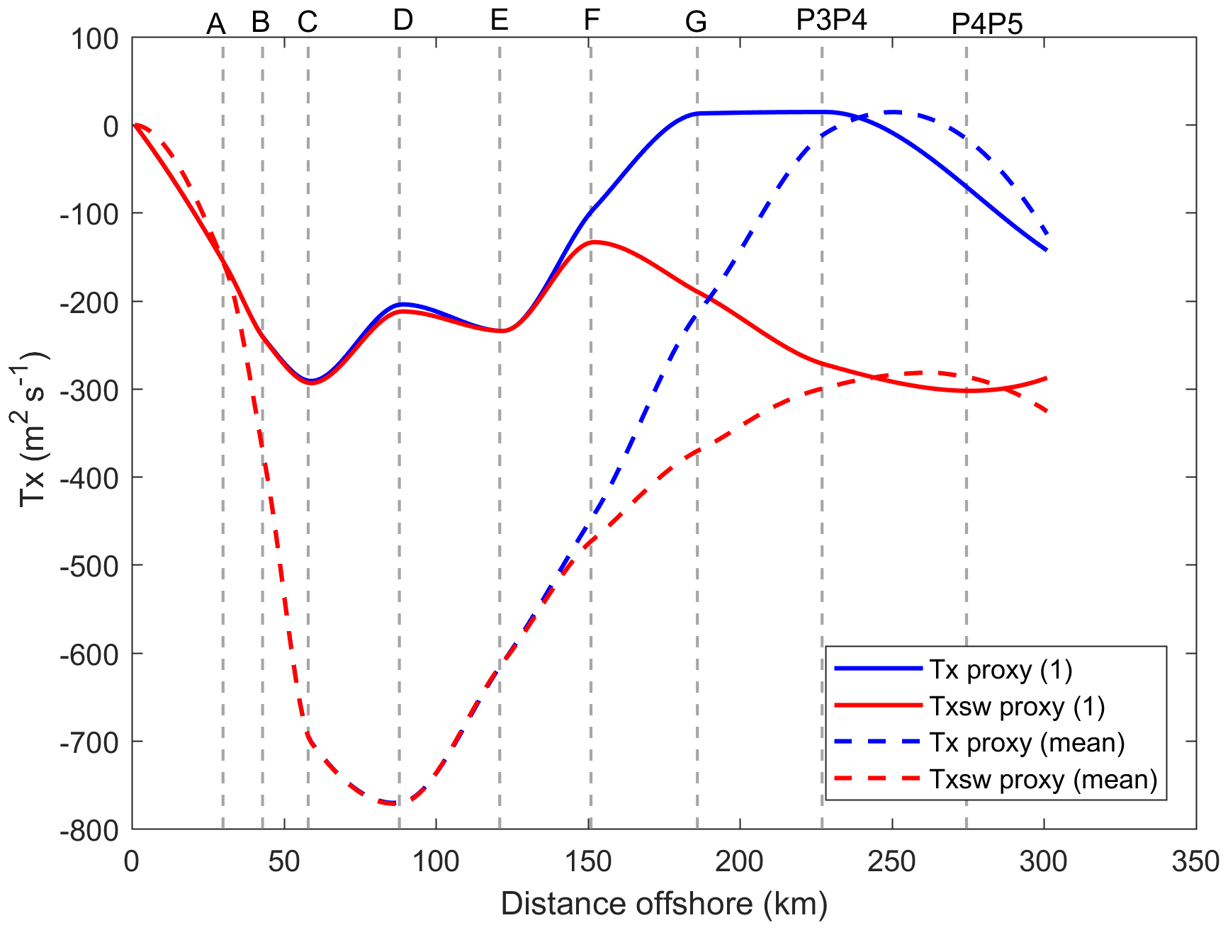
Figure 3HYCOM transport per unit distance proxy (m² s⁻¹) for Tx (blue) and Txsw (red) at 1 km intervals at the first model time step (solid lines) and for the ACT reference period (2010–2013, dashed lines). The dashed grey lines represent the positions of moorings and offshore CPIES pairs.

Download

Assuming that the 3-year linear relationship between SSH slope and transport per unit distance (Tx and Txsw) from 2010–2013 remains constant, the regression models were applied to the entire 34-year SSH model data. Thereafter, the 34-year transports were calculated by applying the same methods that were used to calculate the 3-year transport time series; firstly, obtaining Tx and Txsw estimates at 1 km intervals along the array and secondly integrating horizontally to obtain T_box and T_jet.

2.5 Comparison of the transport proxy to actual model transports

The simulated model transports were calculated using the full-depth velocity fields across the array. If the relationship between SSH slope and transport is strong, there would be good agreement between the proxy and the actual model transports. To quantify this, correlations and transport statistics for the model and proxy were calculated from the two time series (Table 2). These provided insight into which processes the proxy may have failed to capture, which were then further investigated in HYCOM. Statistics are deemed significant at the 95 % significance level.

Eddy kinetic energy (EKE) was calculated to show the surface variability of the current coincident with averaged SSH contours used to represent the mean surface structure (Fig. 6). EKE was calculated over the 3-year mean reference period, and over the highest and lowest correlated years. In order to evaluate the subsurface current structure along the ACT array, vertical velocity profiles were analysed for each mooring and CPIES pair over the 3-year mean reference period as well as over the highest and lowest correlated years.

Transport variability in HYCOM was analysed by investigating the current structure during the residual transport events in the least- and best-performing regression models. Residual transport events were identified as the outlying residual transport values above and below 2 standard deviations of the estimated transport.

where e is the estimated residuals, Txi is the HYCOM transport per unit distance value and $\stackrel{\mathrm{‾}}{\mathrm{Txi}}$ is the estimated transport per unit distance value according to the linear regression models (i.e. the transport proxy).

To investigate the current structure during these residual events, composite averages of the cross-track velocity structure were analysed. The cross-track velocity at each depth layer in HYCOM was extracted at 12 km intervals from 0 to 400 km offshore for the 34-year model period. Although the ACT array only reached 300 km offshore, analysis of the current structure in HYCOM was extended further offshore. Previous analyses have shown increased levels of offshore variability in this HYCOM simulation (Backeberg et al., 2009, 2014), which therefore made it interesting to study the subsurface structure during the offshore current meanders and the influence these could have on the transport proxy. To further investigate the effect of the residual transport values on the transport proxy, all corresponding transport events exceeding plus or minus 2 standard deviations were removed from each linear regression model during development of the proxy (Fig. 4).

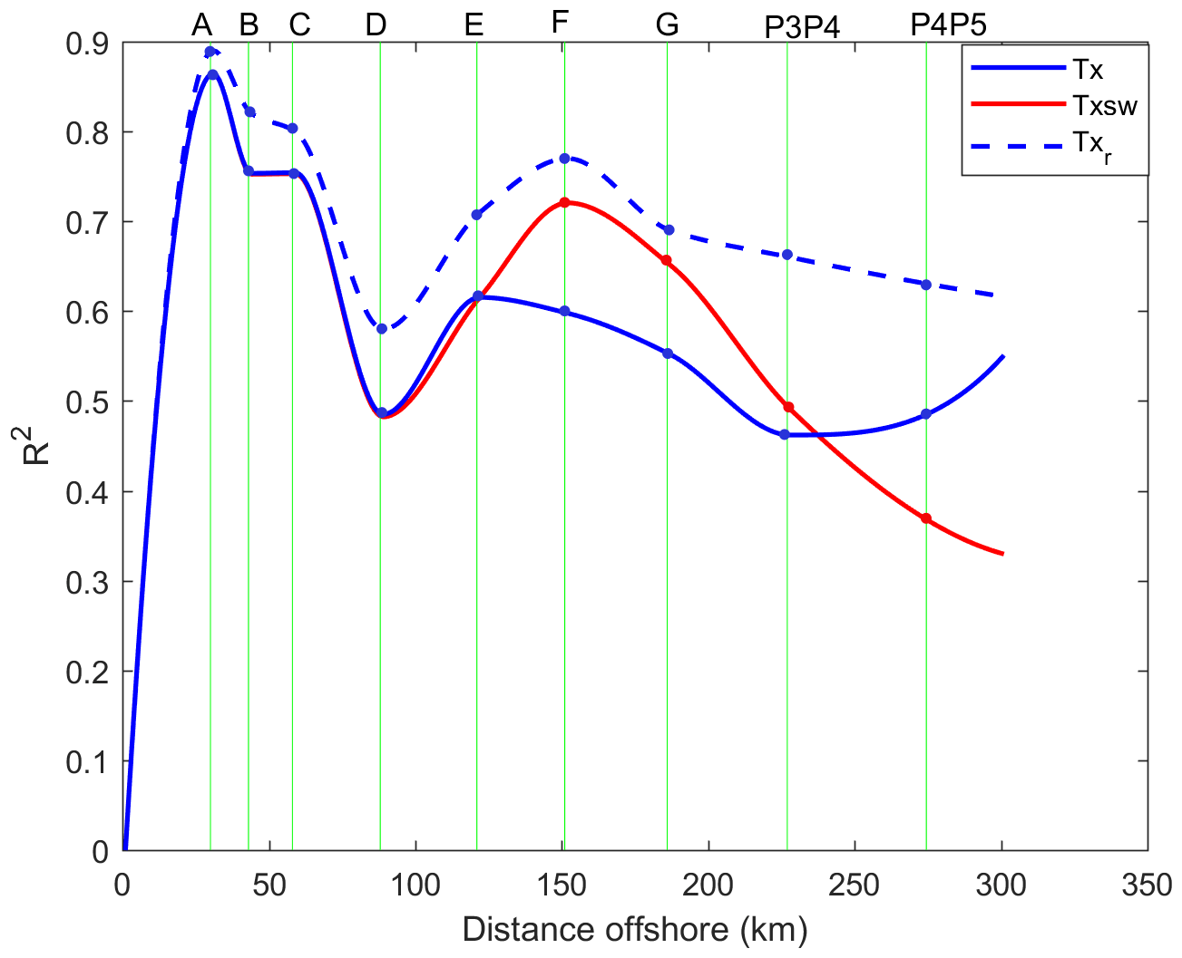
Figure 4R² statistics from the linear regression models showing the relationship between HYCOM SSH slope and HYCOM transport per unit distance for each mooring (A–G) and CPIES pair (P3P4 and P4P5) over the 3-year reference period (2010–2013). Tx is represented by the solid blue line and Txsw by the solid red line. The dashed blue line represents the results of Tx after the removal of the residual transport events (see Sect. 3.4). Sites A to CPIES pair P4P5 are shown by the faint green lines.

Download

2.6 Sensitivity tests

Sensitivity experiments were performed in HYCOM to test how many years of mooring data is needed to create an accurate proxy of Agulhas Current transport. With 34 years of model data the linear relationship could be tested over much longer or shorter periods.

Using the method described in Sect. 2.4.3, the proxy regression models were built using 1, 6, 12, 18, and 34 years of HYCOM data. In addition, the proxies were calculated over two arbitrary 3-year periods to test the sensitivity of the proxy to current dynamics over different years. Lastly, the regression models were calculated over the maximum and minimum annual transport years in HYCOM, as well as during the years the HYCOM transport standard deviation was the largest and the smallest. Table 1 shows the time range over which the sensitivity experiments were performed.

Table 1Sensitivity experiment time periods.

^*Corresponds to the two additional 3-year periods.

Download Print Version | Download XLSX

3.1 HYCOM linear regression models

The coefficients of determination (R²) from the regression models highlight how well the linear relationship predicts the transport in HYCOM (Fig. 4). R² ranged from 0.86 at mooring A (30 km offshore) to 0.49 at the last CPIES pair P4P5 (275 km offshore) for Tx and 0.86 at mooring A to 0.37 at P4P5 for Txsw (P values $<{\mathrm{10}}^{-\mathrm{3}}$). Results from Beal and Elipot (2016) showed an increase in the R² statistics in the regression models ranging from 0.51 at mooring A and 0.81 for CPIES pair P4P5 for Tx, indicating that the in situ observation-based regression models had poorer skill inshore, whereas in HYCOM the regression models have poorer skill offshore. The results from the Txsw regression models in HYCOM showed similar results to Beal and Elipot (2016) for the inshore mooring locations (A, B, C, E) with slightly higher correlations for offshore moorings F, G, and CPIES pair P3P4 but a lower correlation for D and the furthest CPIES pair P4P5.

3.2 Proxy validation

Two transport types, the box transport (T_box) and the jet transport (T_jet), were extracted from HYCOM in order to validate the relative proxies. The T_box (T_jet) proxy explained 57 % (14 %) of transport variance during the 3-year reference period (2010–2013) (Table 2b). Using 34 years of model data (1980–2014), assuming the fixed 3-year relationship between SSH slope and transport, T_box (T_jet) explained 52 % (26 %) of the transport variance (Table 2b). Results from Beal and Elipot (2016) also showed that T_box explained a higher percentage of variance (61 %) during the ACT period than the jet transport proxy (T_jet: 55 %).

Table 2(a) Summary of the transport statistics of the ACT observations over the 3-year in situ period and the HYCOM model transports and HYCOM proxy transports over the 3-year and extended 34-year time periods. Negative values denote transport in the southwest direction. 1 Sv =10⁶ m³ s⁻¹ (sverdrup). (b) Correlations between the HYCOM model transport and HYCOM proxy transport for the box transport and jet transport with the percentage of variance shown in brackets. All correlations were significant.

Download Print Version | Download XLSX

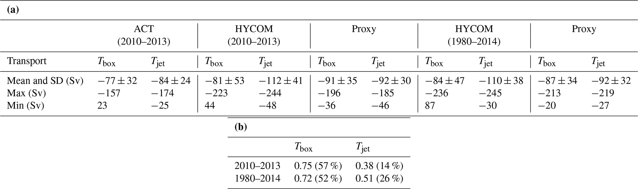
The 34-year mean transport and standard deviation from HYCOM for T_box and T_jet were $-\mathrm{84}\pm \mathrm{47}$ Sv and $-\mathrm{110}\pm \mathrm{38}$ Sv, respectively (Table 2a). The proxy T_box and T_jet were $-\mathrm{87}\pm \mathrm{34}$ Sv and $-\mathrm{92}\pm \mathrm{31}$ Sv, respectively (Table 2a). According to the ACT observations, the mean transport and standard deviation were $-\mathrm{77}\pm \mathrm{32}$ Sv for T_box and $-\mathrm{84}\pm \mathrm{24}$ Sv for T_jet. A higher jet transport was expected considering it excludes northeast counterflows that decrease the box transport (Beal et al., 2015). The differences between the standard deviations of HYCOM and the proxy indicate that transport in HYCOM experiences more variability compared to the proxy. The proxies only capture a portion of the transport estimate from HYCOM, suggesting it also only captures a portion of the model variability. The positive minimum transport values for T_box during both time periods also appear to be peculiar, suggesting a current reversal during those events (Table 2a).

The T_jet annual correlation varies greatly from year to year with a significant maximum correlation of 0.82 (2014) and a minimum correlation of 0.00 (2003) (Fig. 5). In contrast, the correlations for T_box vary much less and are always significant with a maximum correlation of 0.88 (1988) and minimum correlation of 0.50 (1994) (Fig. 5). The box transport has higher correlations for most of the 34-year time period except during two single years where the jet transport has a higher correlation, 0.78 versus 0.70 during 1991 and 0.54 versus 0.50 during 1994. These results indicate that the proxy is generally better suited in HYCOM to estimate the box transport rather than the jet transport.

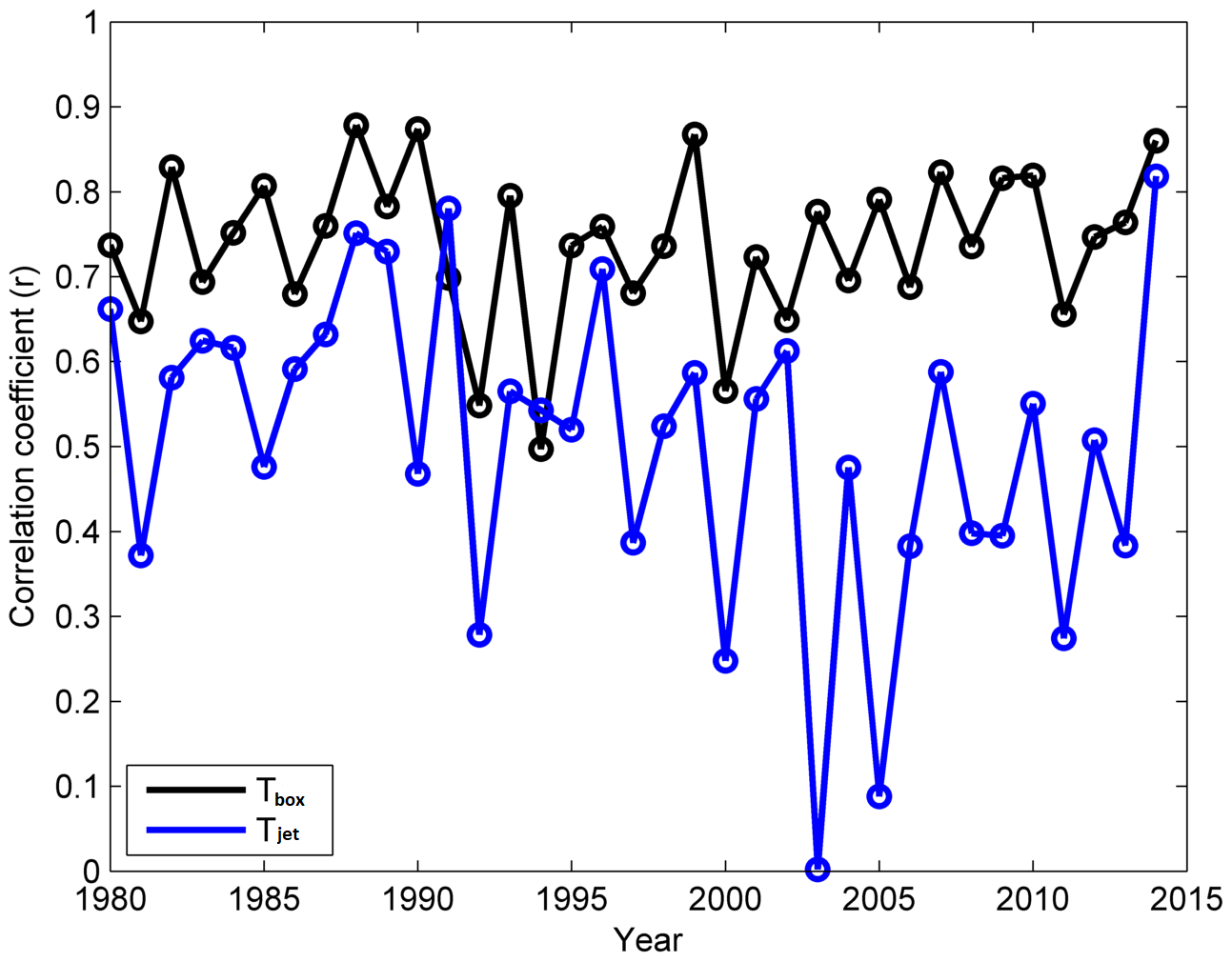
Figure 5This 34-year annual correlations between the box (black) and jet (blue) transport proxies against the box and jet transports extracted from HYCOM.

Download

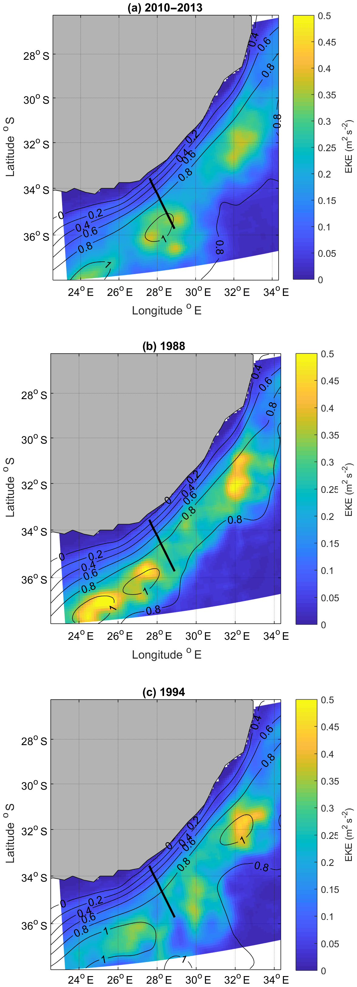
Figure 6Eddy kinetic energy (EKE in m² s⁻²) and sea surface height (SSH in metres) contours during (a) the reference period (2010–2013) (b) the highest (1988), and (c) lowest (1994) correlated years. The black line representing the ACT array.

Download

The jet transport proxy by Beal and Elipot (2016) was developed to estimate the transport of the Agulhas Current during mesoscale meander events, which generally causes the current to manifest as a full-depth, surface intensified, cyclonic circulation out to 150 km from the coast with anticyclonic circulation farther offshore (Elipot and Beal, 2015). The Agulhas meanders in the HYCOM simulation occur in association with large anticyclonic eddies predominantly located at the offshore edge of the current, with a narrow, southwest stream close to the coast (Backeberg et al., 2009). In some instances anticyclonic eddies span the length of the entire array. Therefore, considering that the model is unable to resolve the dynamics associated with meander events, for which the jet transport algorithm was specifically developed, further analysis only focuses on the box transport proxy.

3.3 Evaluating the box transport proxy

The strengths and weaknesses of the box proxy are further investigated by selecting the highest and lowest correlated years from the 34-year annual correlations (Fig. 5), and evaluated by plotting the current structure in the model over the respective years (Figs. 6 and 7).

During the year with maximum correlation (1988) the current is stable and inshore, whereas during the lowest correlated year (1994) and during the proxy reference period (2010–2013) the current is meandering and it appears that a large portion of the energy of the current has been shifted offshore (Fig. 6). The narrow spacing of the SSH contours for all three periods indicates a strong gradient inshore and hence a strong mean geostrophic current; however, the wide spacing between the SSH contours offshore suggests that the variability in the model is confined to the offshore side of the current. It is assumed that high levels of mesoscale variability in the model could bias the current position and hence the transport estimate. However, based on the analysis there were approximately five anticyclonic eddies during the highest correlated year (1988) and approximately seven anticyclonic eddies during the lowest correlated year (1994) which does not explain the difference in the accuracy of the proxy for those years.

The model cross-track velocity changes direction with depth, specifically for offshore mooring G and CPIES pairs P3P4 and P4P5 at the depth of ∼2000 m (Fig. 7), thereby defining the depth of the Agulhas jet. During the 3-year reference period the velocity changes direction at moorings B and G (∼1200 and ∼2000 m, respectively) and at sites P3P4 (∼2000 m) and P4P5 (∼300, ∼2000 m). During 1988, sites F–P4P5 experience a change in direction (≳2000 m). Lastly, during 1994 mooring G and sites P3P4 and P4P5 exhibited a change in direction (≳2000 m). An explanation for the offshore subsurface countercurrents may be due to the impinging baroclinic eddies continuously propagating downstream (Backeberg et al., 2009), affecting the entire water column by changing the direction of flow at certain depths. This directly impacts the accuracy of the proxy and explains why the transport proxy fails to capture current reversals (Table 2), because the SSH slope does not capture the subsurface countercurrents associated with the impinging baroclinic eddies.

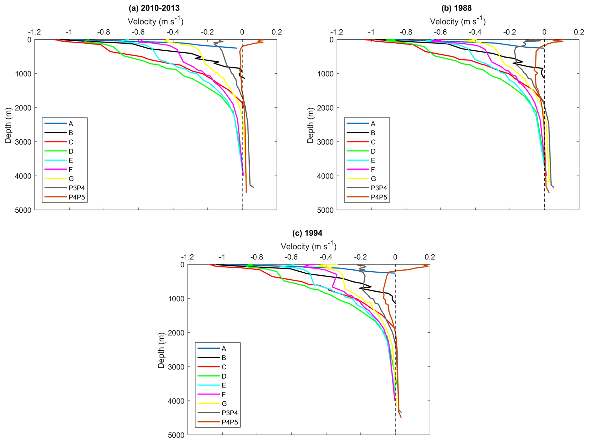
Figure 7Mean cross-track velocity profiles (m s⁻¹) during (a) the 3-year reference period (2010–2013), (b) during the highest correlated year (1988), and (c) the lowest correlated year (1994). Each colour represents the different moorings (A–G) and CPIES pairs (P3P4 and P4P5). Negative values indicate southwestward flow.

Download

3.4 Investigating the transport variability

As shown previously, the performance of the linear regression models weakened moving offshore (Fig. 4). Regression model RM8 (CPIES pair P3P4, Fig. 8a) captured the least transport variance at 46 % and RM 1 (mooring A, Fig. 8b) explained the most transport variance at 86 %. According to our methods, a negative SSH slope in HYCOM corresponds to a negative (southwestward) surface velocity; and if the current structure were barotropic, a negative (southwestward) transport and vice versa.

As shown in RM 1 (Fig. 8b), all the data points are clustered such that the negative SSH slope relates to a negative Tx value, in the absence of northeast counterflows. Careful analyses of RM 8 indicates that eight of the nine residual transport events violate the proportional relationship between SSH slope and Tx (Fig. 8a). Some of which have a negative SSH slope relating to a positive Tx value where others show a positive SSH slope with negative Tx value. Therefore the SSH slope does not always reflect the direction of flow at depth, and thus the correct sign for Tx.

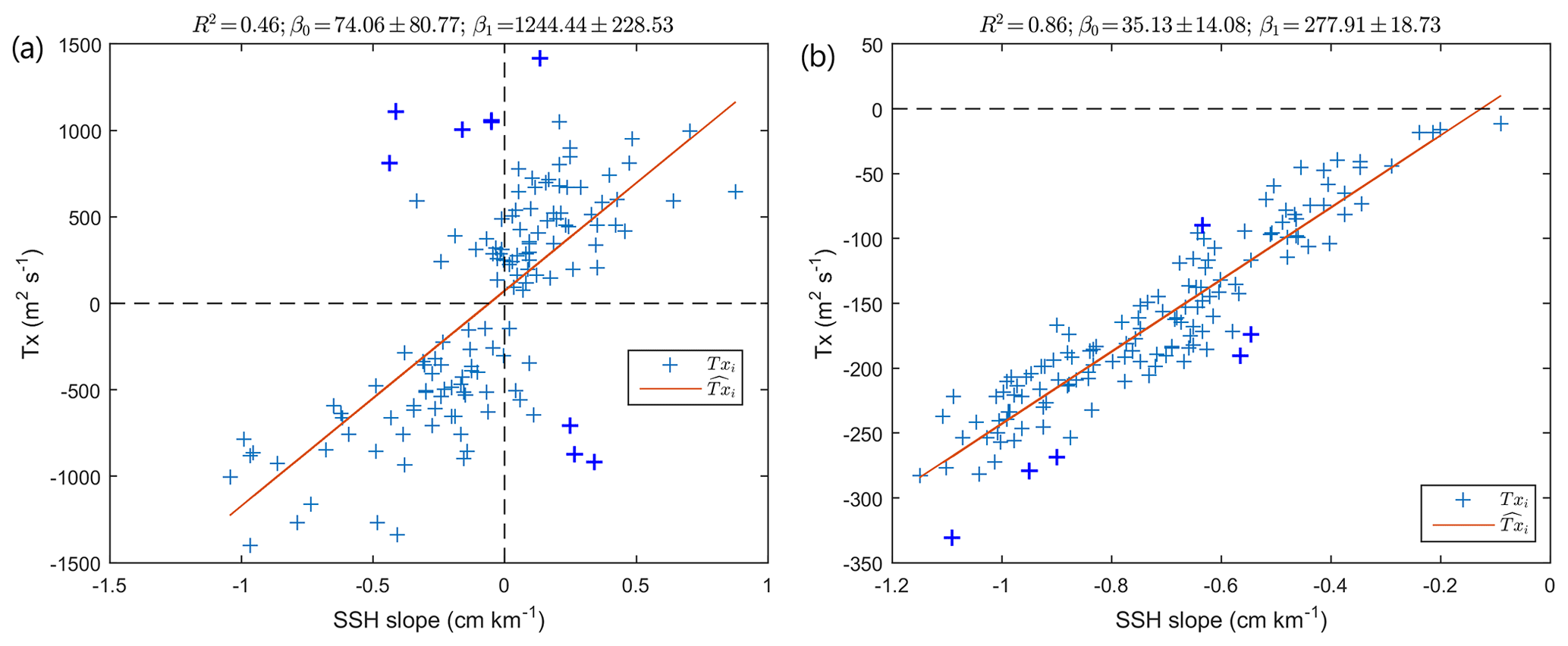
Figure 8Linear regression models showing the relationship between HYCOM SSH and transport per unit distance (Tx) for (a) RM 8, capturing the least transport variance (46 %), and (b) RM 1, capturing the most transport variance (86 %). Txi (blue crosses) represent the Tx values from HYCOM and $\stackrel{\mathrm{‾}}{\mathrm{Txi}}$ (red line) represents the Tx estimates from the linear regression model. The bold crosses highlight the residual transport events with transport values greater or less than 2 standard deviations of the transport estimate. The coefficient of determination (R²) quantifies the amount of variance explained by the regression model; β₀ is the slope coefficient and β₁ the intercept with 95 % confidence intervals. Note the different scaling on the x and y axes.

Download

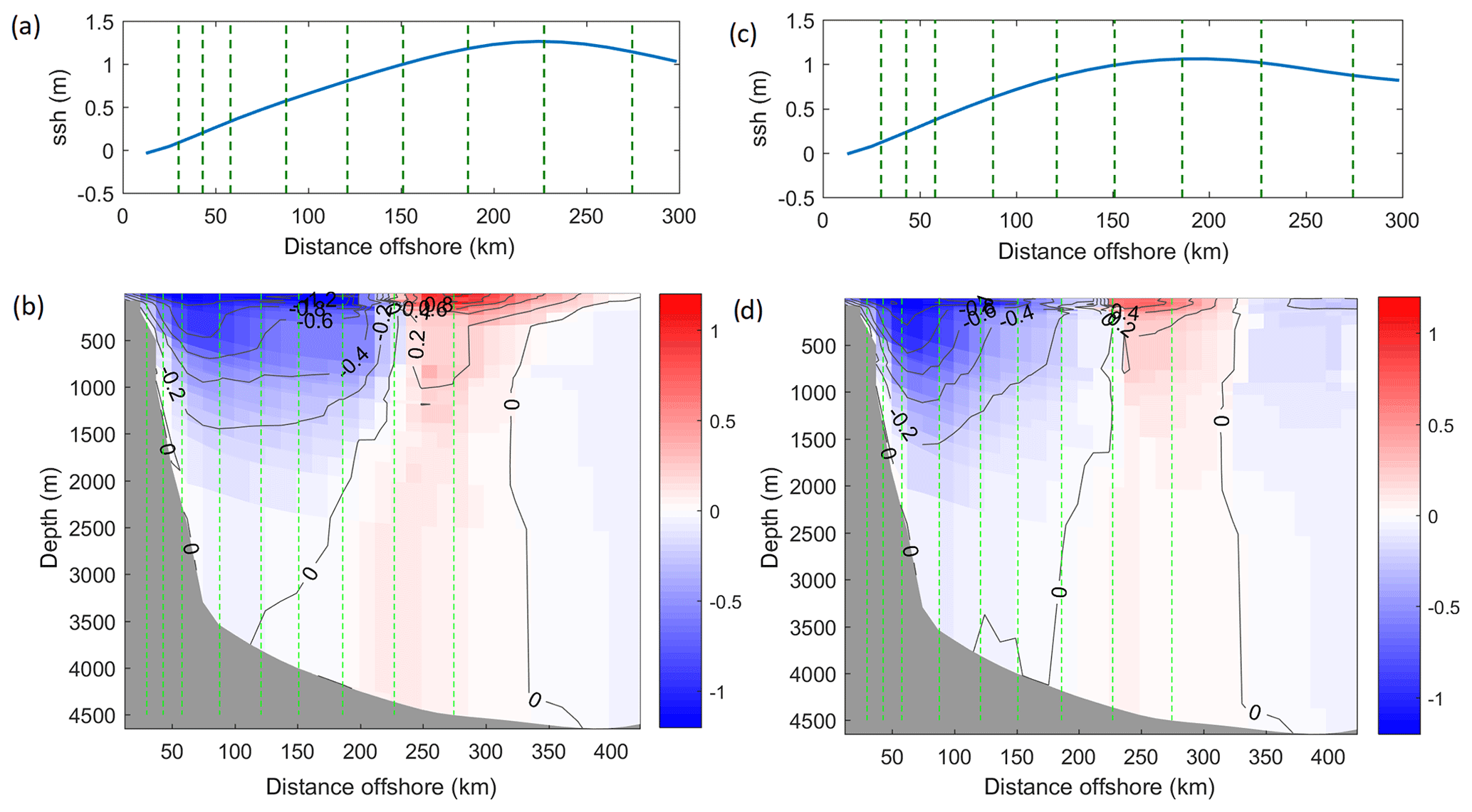
Figure 9Mean SSH (metres, m) and composite cross-track velocity structure (metres per second, m s⁻¹) of the residual transport events from RM 8 (a, b) and RM 1 (c, d). Blue shading represents the negative, southwest current flow and red represents the positive, northeast current flow. Contours are every 0.2 m s⁻¹. Dashed vertical lines represents the nine locations of the mooring and CPIES pairs, the first line representing mooring A and CPIES pair P4P5 furthest offshore.

Download

It was expected that removing the outlying transport events (outliers larger than ±2 standard deviations) would increase the statistical performance of the linear regression models (Fig. 4). However, it is noteworthy that the improvement was remarkably better for the offshore regression models since the baroclinic eddies responsible for breaking down the linear relationship between SSH slope and transport frequently effected the offshore edge of the current.

Examination of the composite cross-track velocity structure of the residual transport events (Fig. 9) shows that there is a change in the direction of velocity in the bottom layers at the location of RM 8 (CPIES pair P3P4). The cross-track flow in the surface layers (∼0–700 m) of the current is southwestward, whereas below ∼700 m the flow is northeastward. Therefore, the vertically integrated flow (Tx) is positive (northeastward) and in the opposite direction implied by the SSH slope. In contrast, at mooring A (RM 1), the composite velocity field is always southwestward, consistent with the SSH slope.

3.5 Sensitivity tests

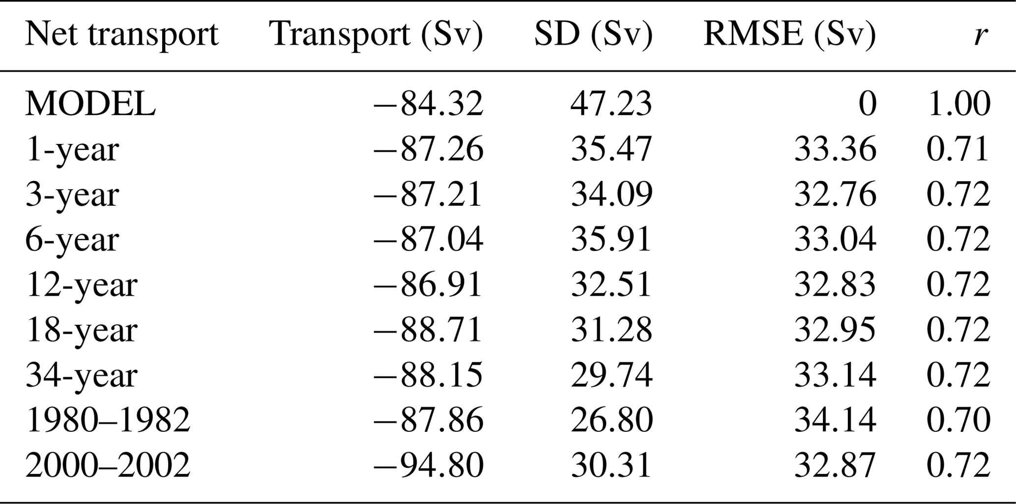
The 34-year Agulhas transport proxy under analysis thus far was based on regression models built using only 3 years of HYCOM model data. The statistics in Table 3 show the results obtained from building the linear regression models and deriving the transport proxy using 1, 3, 6, 12, 18, and 34 years of model data. We find that the correlation between proxy box transport and model box transport is not improved by using more years of model data to build the proxy. Using data from 2010 to 2013 the correlation of 0.72 changes by no more than 0.01 when extending the number of years of model data (Table 3). Similarly, building the proxy with 1 year of model data decreases the correlation by only 0.01 (Table 3). The only difference was the decrease in standard deviation.

The sensitivity of the box transport proxy was also tested using two arbitrary 3-year periods. In comparison to the correlation obtained during 2010–2013 the correlation decreased by 0.02 during 1980–1982 and remained the same during 2000–2002. The results obtained from calculating the T_box proxy during the maximum (minimum) transport and standard deviation years in HYCOM showed no improvement or decrease in the skill of the proxy either.

Table 3Transport statistics and correlation results obtained from calculating the box transport proxy over a range of time periods.

Download Print Version | Download XLSX