the Creative Commons Attribution 4.0 License.
the Creative Commons Attribution 4.0 License.
 | 05 Jun 2019
The long-term variability of extreme sea levels in the German Bight
Andreas Lang
Uwe Mikolajewicz
Extreme high sea levels (ESLs) caused by storm floods constitute a major hazard for coastal regions. We here quantify their long-term variability in the southern German Bight using simulations covering the last 1000 years. To this end, global earth system model simulations from the PMIP3 past1000 project are dynamically scaled down with a regionally coupled climate system model focusing on the North Sea. This approach provides an unprecedented long high-resolution data record that can extend the knowledge of ESL variability based on observations, and allows for the identification of associated large-scale forcing mechanisms in the climate system.
While the statistics of simulated ESLs compare well with observations from the tide gauge record at Cuxhaven, we find that simulated ESLs show large variations on interannual to centennial timescales without preferred oscillation periods. As a result of this high internal variability, ESL variations appear to a large extent decoupled from those of the background sea level, and mask any potential signals from solar or volcanic forcing. Comparison with large-scale climate variability shows that periods of high ESL are associated with a sea level pressure dipole between northeastern Scandinavia and the Gulf of Biscay. While this large-scale circulation regime applies to enhanced ESL in the wider region, it differs from the North Atlantic Oscillation pattern that has often been linked to periods of elevated background sea level.
The high internal variability with large multidecadal to centennial variations emphasizes the inherent uncertainties related to traditional extreme value estimates based on short data subsets, which fail to account for such long-term variations. We conclude that ESL variations as well as existing estimates of future changes are likely to be dominated by internal variability rather than climate change signals. Thus, larger ensemble simulations will be required to assess future flood risks.
- Article
(3206 KB) -
Supplement
(1080 KB) - BibTeX
- EndNote


Inundation due to storm floods is one of the major geophysical risks in coastal regions and bears high damage potential for coastal environments, in both natural and socioeconomic terms. This is especially important for low-lying regions such as coasts and estuaries of the southern North Sea and, in particular, the German Bight. Situated between Denmark to the north and the Netherlands to the west, the German Bight is a shallow shelf sea under the influence of the major northern hemispheric storm-track paths. At the same time, the shallow water depths of under approximately 40 m (see Fig. 1) in combination with the basin's geometry lead to relatively strong tides, with a maximum tidal range of around 4.5 m. Thus, storms can generate particularly high floods in this region. The region has seen many devastating storm floods in the past: one of the most severe, the great storm flood “Grosse Manndrenke” (the Great Drowning of Men) in 1362, resulted in death tolls of tens of thousands, the destruction of numerous settlements including the disappearance of the legendary town “Rungholdt” (Heimreich, 1819), and shifts in the Wadden Sea coastline (Hadler et al., 2018). More recently, the great flood in 1962 resulted in a high death toll and vast economic loss along the coastal regions of Germany and in particular the city of Hamburg. Disasters like these have driven extensive research in the field; yet, most studies focused on individual events, on the observed trend during the last couple of decades, or a projection of future storm flood exposure. Variations on longer timescales and their underlying mechanisms have received less attention. However, a deeper understanding of the long-term variability of strength and occurrence of extreme storm floods can be of great importance for coastal planning and risk assessment. Here we assess the longer-term variability of high sea level extremes in the German Bight using a novel regionally coupled model approach over a 1000-year-long simulation period.
Following Pugh and Woodworth (2014), the sea level at a certain point and time can be decomposed into three factors: meteorological surge, astronomical tide, and background sea level (BSL). The surge is the “dynamic response of the sea surface to forcing by the atmosphere” (Mawdsley and Haigh, 2016) and can consist of (i) the local wind surge that pushes water against the coast, (ii) an external surge generated in the North Atlantic by fast bypassing cyclones and air pressure variations that travel as a Kelvin wave counterclockwise in the North Sea (Gönnert and Sossidi, 2011), and (iii) the direct effect of air pressure acting on the water surface (the inverse barometric effect). The total sea level is thus a product of interactions between the surge component, the astronomical tide, and the underlying longer-term change in BSL, the latter of which depends on various oceanographic and atmospheric processes such as coastally trapped waves, local steric effects, or alongshore winds (Dangendorf et al., 2014a; Sturges and Douglas, 2011; Calafat et al., 2012). Extreme sea levels particularly arise when these components are in superposition, e.g. if a strong wind surge occurs concomitantly with a tidal maximum, or – as a result of the tide-surge interaction – a few hours before on the rising tide (Horsburgh and Wilson, 2007). Topographic features, such as water depth, sand bars, or reefs can further affect their height locally. These components interact nonlinearly (e.g., Kauker and von Storch, 2000; Plüß, 2004) and are nonstationary, with variations occurring on multiple timescales. Long-term changes in any of those components, e.g. due to internal variability or external climate change, may substantially alter the risk associated with sea level extremes. Since we are solely interested in high water extremes, we refer to them with the term extreme sea level (ESL) but only to the upper end of the distribution.

Figure 1Bathymetry of the North Sea (a) and the German Bight (b; the main study location, Cuxhaven, is marked by the black square) as represented in MPIOM. The model's land mask is shown in white and the present-day coastline is shown in black.
Many studies have investigated the recent dynamics of ESL both regionally and globally using data from tide gauges (e.g., Tsimplis and Woodworth, 1994; von Storch and Reichardt, 1997; Woodworth and Blackman, 2004; Marcos et al., 2009; Menéndez and Woodworth, 2010; Mudersbach et al., 2013; Weisse et al., 2014; Wahl and Chambers, 2015) or using barotropic surge models for hindcasts of storm surges (e.g., Kauker and von Storch, 2000; Langenberg et al., 1999; Woth, 2005; Weisse and Plüß, 2006). For a review of past storm surge statistics and projected changes in the North Sea region see Weisse et al. (2012). While most studies agreed on an overall increase in storm surge activity along the German Bight since the 1960s (e.g., WASA-group, 1998; Weisse and Plüß, 2006; von Storch and Woth, 2008; Mudersbach et al., 2013), both observations and hindcast simulations over a longer time span have set this recent trend into the perspective of a marked multidecadal variability during the last century (e.g., WASA-group, 1998; Dangendorf et al., 2013b; Mudersbach et al., 2013; Weisse and Plüß, 2006) with higher values at the beginning and end of the century.
The data record, though, is limited and only few high-frequency tide gauge records (e.g. Cuxhaven) date back more than a couple of decades. Thus, conclusions on multidecadal to centennial variability as well as the separation of longer-term fluctuations from the transient sea level rise are difficult from a statistical point of view. Concerning the latter, different studies on German Bight sea level reported similar ESL and BSL trends (e.g. Kauker and Langenberg, 2000) or trends at rather different rates (e.g., Mudersbach et al., 2013; Dangendorf et al., 2014b) – a question of great importance for estimations of future ESL behavior on top of a gradual sea level rise. Furthermore, as ESLs are by definition rare, the attribution to modes of climate variability, which often operate on similar or even longer timescales, is hampered by the short instrumental record. While many studies have related mean sea level variations to modes of climate variability – especially the North Atlantic Oscillation (NAO) (e.g., Wakelin et al., 2003; Dangendorf et al., 2012; Ezer et al., 2015), the dominant pattern of atmospheric variability over the North Atlantic (Hurrell, 1995), which showed coherent trends during the last decades – only a few have set this into context with ESL variations (Woodworth and Blackman, 2004; Woodworth et al., 2007; Marcos et al., 2009; Marcos and Woodworth, 2017). Finally, such long-term ESL fluctuations can also have important implications for storm flood protection measures. The design of coastal defense structures in Germany is based on deterministic or statistical approaches (e.g. Ministerium für ländliche Räume des Landes Schleswig-Holstein, 2012). For the latter, water levels with assigned return periods are needed, which are typically based on parametric extreme value analysis of observed sea level data. Yet, due to the relatively short tide gauge records, the quality of the estimation of return periods longer than the investigated sea level data series depends on the type of extreme value distribution and its goodness of fit to the data. Additionally, any longer-term variability in ESLs further complicates the estimation of high return levels, as they depend on the state of long-term variability during the underlying baseline period. Here we argue that significant centennial variations in high-impact return levels entail a large source of uncertainty for parametric ESL estimates. The standard approach using a typically short baseline period for such sea level estimates thus fails to reflect the possible range of most extreme events that happen only once or twice during that period.
A longer, frequent data series as obtained from a climate simulation can offer a statistically more robust assessment of these problems, as the full time series can be treated as an ensemble of data series comparable in size to the observational record. However, currently available long-term climate simulations do not include tides and have an insufficient resolution to realistically represent storm surges in the North Sea. Dynamical surge models or regional climate models, driven by global climate model simulations, can provide a better representation of small-scale processes, topographic influences, and land–sea contrasts, and are thus better suited for the simulation of extreme events. Due to their open lateral boundaries, however, they cannot account for a consistent propagation of external signals into the study region, which has been shown to affect North Sea sea level variability (e.g., Chen et al., 2014). Here we employ a global ocean model with regionally high horizontal resolution, which allows a consistent simulation of signals propagating from the open Atlantic onto the northwest European Shelf, coupled to an atmospheric regional model to dynamically downscale the climate variations from a Last Millennium simulation from MPI-ESM (Jungclaus et al., 2014; Moreno-Chamarro et al., 2017). With a long-term simulation, this study allows for a nonparametric approach in estimating such high return levels and can thus give insight into the uncertainties in extreme value analysis when based on short records. The goal is to describe and understand the (multi)decadal variability of ESL in the German Bight as well as their relationship with BSL and large-scale climate variability, which to our knowledge has not yet been investigated in a model study over such long timescales.
This article is structured as follows: Sect. 2 introduces the model system and experimental setup. In Sect. 3, we present results on ESL variability, including the validation of the model with respect to observations from tide gauges (Sect. 3.1), the relation to BSL (Sect. 3.2), and climate variability (Sect. 3.3). The results on ESL variability as well as some implications for observation-based extreme value estimates are discussed in Sect. 4. Finally, in Sect. 5 we close with a summary and conclusions for coastal defense measures.
2.1 Model system and experimental design
This study employs a regionally coupled climate system model, consisting of the global ocean model MPIOM (Marsland et al., 2004; Jungclaus et al., 2013) and the regional atmospheric model REMO (Jacob and Podzun, 1997). Both models are interactively coupled over the wider EURO-CORDEX domain (e.g., Jacob et al., 2014) with the coupler OASIS-3 (Valcke, 2013). The coupled model system has been described in Mikolajewicz et al. (2005); Elizalde et al. (2014); and Sein et al. (2015); a sketch is shown in Fig. 2.
REMO is run with a 0.44∘ setup, corresponding to approx. 50 km grid spacing, and with 27 vertical levels covering Europe, northern Africa, and the northeast Atlantic. MPIOM is run on a stretched grid configuration with a nominal horizontal grid resolution of 1.5∘ and 30 vertical layers. In order to maximize the grid resolution in the study focus area, the model's poles are shifted to central Europe and North America, respectively. This results in a maximum grid resolution of under 10 km in the German Bight and thus enables a more realistic simulation of small-scale shelf processes. Furthermore, it includes the full lunisolar tidal potential according to Thomas et al. (2001). At the same time, the ocean model's global domain without lateral boundaries allows for the full simulation of signals propagating from the open Atlantic into the North Sea. In order to prevent ocean grid points falling dry due to strong tidal sea level variations, e.g., in the English Channel, MPIOM's uppermost layer thickness is set to 16 m. This model setup is identical to the one used in Mathis et al. (2018).

We employ this model setup to downscale transient coupled climate simulations performed with the paleo version of the global earth system model MPI-ESM (Max-Planck-Institute Earth System Model) in its low-resolution (LR) version (Giorgetta et al., 2012), corresponding to 1.875∘ or approx. 200 km grid spacing in the atmosphere. The parent global simulations cover the period 900–2000 CE and comprise parts of the PMIP3 simulation Last Millennium (850–1850 CE; Jungclaus et al., 2014; Moreno-Chamarro et al., 2017), extended with the corresponding CMIP5 “historical” simulation (1850–2005 CE Taylor et al., 2012), including all relevant transient forcings. Greenhouse gases (GHGs) follow the PMIP3 protocol (Schmidt et al., 2012), solar irradiance is prescribed after Wang et al. (2005), and volcanic eruptions in terms of radiation imbalance after Crowley et al. (2008) (see Supplement Fig. S3). six-hourly atmospheric forcing derived from the atmosphere component of the driving general circulation model (GCM) is used as lateral boundary conditions for REMO, or as surface forcing for MPIOM outside the coupling domain. Topography and coastlines as well as ice sheets are immutable, and thus transient sea level modulations due to ice sheet melt or changes in coastal morphology including land sinking or lifting are not accounted for. Furthermore, as a Boussinesq model, MPIOM conserves volume rather than mass and therefore does not explicitly represent the thermosteric sea level rise.
The downscaling was performed as one continuous run with hourly coupling started in year 900 CE, the first 100 years are used as a spin-up. Sea level and selected atmospheric fields are stored at hourly resolution. Additionally, in order to quantify the variability from the downscaling process, as well as the contributions of natural variability and external forcing, we performed two further downscalings: one of the same global realization and one of another ensemble member of the global Last Millennium simulations, each starting in 1400 CE, with the first 100 years again used as spin-up (see the Supplement S3). The implications of these additional downscalings are discussed in the respective sections; yet, for simplicity, we only show results from the 1000-year continuous downscaling.
2.2 Extreme value sampling
Several techniques have been used to characterize extreme sea level, e.g. the use of high percentiles (e.g., Woodworth and Blackman, 2004; Dangendorf et al., 2013a), the selection of r-largest maxima over a block of time (e.g., Araújo and Pugh, 2008; Méndez et al., 2007; Marcos et al., 2009), and the selection of peaks over a certain threshold (POT) (e.g., Méndez et al., 2006). While the choice of the respective percentile, threshold, block length, or number of block maxima is essentially arbitrary, the resulting events are sensitive to the choice of extreme value sampling index which represents a trade-off between bias (too high r or too low threshold) and variance (too low r or too high threshold) of the estimates.
Here, we have chosen the annual maximum sea level as an index representing ESL. Due to its relative definition of what constitutes an extreme, it is robust to temporal variations. The use of a “direct” method for ESL (instead of, for example, surge residual or skew surge) is chosen in order to avoid a decomposition between tidal and surge parts and their nonlinear interaction. Since storm floods primarily occur in winter, annual statistics are computed for years defined as starting in July and ending in June in order to not split up one storm flood season. If not specified otherwise, these definitions are used when referring to ESL in the text.
For the design of coastal defense structures, policy makers and adaptation planners often require statistics of water levels of a certain assigned return period (e.g. Ministerium für ländliche Räume des Landes Schleswig-Holstein, 2012), especially those of high impact but low probability, i.e. the upper tail. The return periods and associated exceedance probabilities are typically estimated based on parametric extreme value analysis of the available instrumental data record. As data records rarely date back more than a couple of decades, this implies a substantial extrapolation of the data. That is, in order to obtain estimates for large return periods, different extreme value distributions are fitted to the comparably short data series. The choice of extreme value distribution depends on the considered extreme value sampling method and ultimately represents a trade-off between bias and variance of selected extremes. While the POT method is linked to the generalized Pareto distribution, the r-largest samples follow approximately a three-parameter generalized extreme value (GEV) distribution (e.g., Coles et al., 2001). Its cumulative distribution function is
where F is the probability that a water level z will not be exceeded, while μ, σ, and k are the location, scale, and shape parameters, respectively. The special cases for k=0, k<0, and k>0 represent three extreme value families, namely the Gumbel (type I), Weibull (type II) and Fréchet (type III) distributions (Coles et al., 2001). From Eq. (1), the probability of exceedance is , where E(z) represents the expected frequency of events exceeding z. The expected time interval between events of level z or greater, the return period (RP), is
The advantage of our long simulation period is that it allows us to infer high-end extreme value statistics without the use of parametric methods. These nonparametric estimates have been inferred by first ranking the data points of the sea level time series and associating a cumulative probability to each value. The probability of exceedance is , where m is the rank of N observations ordered in decreasing order. Following Eq. (2), return periods are again defined as the reciprocal of the respective probability of exceedance.
The simulated times series of ESL at Cuxhaven (see Fig. 1) over the last 1000 years is shown in Fig. 3 (black curve). For comparison, we show the frequency of storm floods as events binned per decade (blue), following the storm surge definition from the Federal Maritime and Hydrographic Agency (BSH) (Müller-Navarra et al., 2003). Heavy (extreme) storm floods correspond to elevations above 2.5 (3.5) m relative to the long-term mean high water level (MHW). The BSL as a reference in terms of winter median is shown in green. Sea level is given in meters above the long-term mean and the model location of Cuxhaven refers to its nearest grid point.
Simulated ESLs range between 2 and 5.5 m above the long-term mean. With a standard deviation of 50 cm and a maximum year-to-year amplitude of roughly 3 m, ESLs exhibit large interannual variations and pronounced variability on various timescales. Yet, the highest events occur without pronounced clustering throughout the full 1000 years. This variability is analyzed in more detail below.

Figure 3Simulated ESL (black), winter median sea level (green) and number of heavy (blue bars) and extreme (dark blue bars) storm surges per decade at Cuxhaven. Thick lines denote the 11-year running mean.
3.1 Validation of simulated storm surge statistics
As the reality can be viewed as only one realization of the climate system one should not compare individual historic events in simulation and observation, but rather their statistics. To validate the model's performance considering storm flood statistics, we compare the simulated ESLs with observations from the tide gauge record in the German Bight (data from the AMSeL project, see Jensen et al., 2011; Wahl et al., 2011), and specifically show results at Cuxhaven which, starting in 1900, marks one of the longest reaching records of the German Bight tide gauge stations. The long-term (linear) trend in the tide gauge data has been removed.
While the general North Sea tidal oscillations are well-reflected in the model, the tidal range is underrepresented at Cuxhaven (see Fig. S1 for a comparison of the broader highest water level from observations and model simulation). Accordingly, this results in a lower long-term MHW (defined as the temporal mean over tidal maximum values). Relative to the respective long-term MHW, however, simulated and observed ESLs compare well (see the quantile plot in Fig. 4 for ten 100-year-long segments of the simulation against the Cuxhaven tide gauge record.), and we therefore express ESL in such relative terms in the remainder of the study.
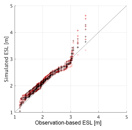
Figure 4Quantile–quantile plot of simulated sea level at Cuxhaven against the 100-year-long ESLs from the tide gauge record. Colors following the gradient from light red to black represent ascending 100-year segments from 1000–2000.
Figure 5 shows return values of ESL compared to the Cuxhaven tide gauge record. In order to better compare the different data record lengths, the simulated 1000 years of data are again split into ten 100 year-long segments, roughly the length of the Cuxhaven tide gauge record. Both slope and magnitude above MHW are well-captured; the return values inferred from observations lie within the spread of the model simulation at all periods. Yet, other than in the simulation, observations tend to level off for return periods above 20 years, before they rise again for return periods higher than 50 years, while simulated return levels rather increase steadily. As a consequence, the 100-year return levels (RL100) in all but the 11th century exceed the corresponding return water level inferred from the instrumental record. The large scatter of about 1.2 m between the highest simulated sea levels of each century has important implications for extreme value analysis (see Sect. 4).
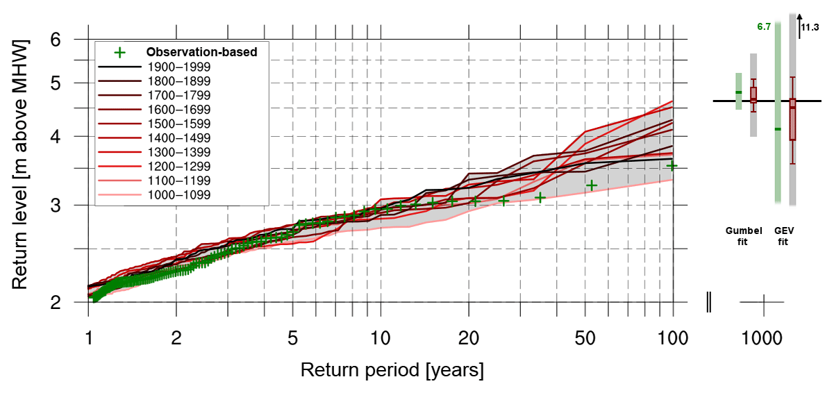
Figure 5Return value plot using nonparametric plotting positions of simulated sea level at Cuxhaven (colored lines represent 100-year-long subsets of the full 1000 years) against observations from tide gauges (green crosses). The bars on the right mark the corresponding RL1000 estimates using a Gumbel (left) and GEV (right) fit to the observations (dark green, 95 % confidence interval in light green) and to each 100-year subset of the simulation (red box-whiskers, range of the 95 % confidence intervals in grey). The horizontal black line shows the RL1000 directly inferred from the full simulation.
The spatial structure of simulated return values (Fig. 6) shows lowest values for open waters which increase towards the coast, especially the inner German Bight. Most points along the German Bight coast (circles represent Cuxhaven; Husum; Norderney; and Delfzijl, Netherlands) compare well with the respective tide gauge records. Yet, while the return values at Cuxhaven lie slightly higher than the observed ones, ESLs along the coastline of Lower Saxony and the Netherlands are rather low compared to the observation-based estimates. Furthermore, the model's uppermost layer thickness is 16 m well above the shallow shorelines of the Wadden Sea (see Fig. 1) and thus likely leads to lower surge heights. Note that for Husum and Norderney the observational record does not date back the full 100 years, so these points are only shown for the 50-year return period.

Figure 6Gridded 50- and 100-year return levels and the corresponding water values from tide gauge observations at selected locations (circles). All values given in meters above mean high water.
The seasonality is well-captured, with strongest and most frequent storm floods in winter (Fig. S2), especially in the months of October–January. However, the distribution is slightly shifted towards autumn and early winter.
In agreement with observational studies (Gerber et al., 2016), simulated storm floods at Cuxhaven stem from predominantly west-northwesterly directions, while their associated daily pressure anomaly patterns (not shown) are similar to observations of storm flood weather situations (Donat et al., 2010; Dangendorf et al., 2014c).
We thus conclude that the model reasonably reproduces storm flood physics and statistics. Due to the good skill in reproducing storm surge statistics as well as the comparability owing to its relatively long instrumental record, the remainder of this study will focus on Cuxhaven only. However, the temporal variability in other grid points along the German Bight is similar (see Fig. S6) and the results discussed here qualitatively agree irrespective of the exact location.
3.2 Relation to the background state
An important question concerning ESL variability as well as future ESL projections is the relation to time-averaged sea levels, i.e. the background state. Separation into the different components of extreme water levels, such as the subtraction of mean and tide are useful methods to investigate this question (e.g. Woodworth and Blackman, 2004). Reviewing literature on recent ESL trends globally, Woodworth et al. (2011) concluded that the majority of studies suggest an increase over the last century, but at rates comparable to those observed in BSL at most locations. However, analyzing tide gauge records in the German Bight, Mudersbach et al. (2013) found differences in linear trends in high sea level percentiles from those in mean sea level. Are these differences representative for this period only or can the finding be extended to a general statement?
Figure 3 shows both ESL in terms of annual maxima (black) and BSL in terms of winter median sea level (green), and their respective 11-year running mean. We choose the median instead of the more simple mean in order to avoid a skewed value due to an exaggerated influence of the tails of the distribution. As the predominant storm surge season, we only average over an extended winter period (October–March). Neither ESL nor BSL exhibit long-term trends, but show high interannual to multidecadal variability. Yet, their modulations are not always coherent: as the histogram at the bottom of Fig. 3 shows, years with one extreme storm surge do not necessarily coincide with a greater occurrence of more moderate heavy storm floods or elevated BSL. The correlation between BSL and ESL is comparably low (r=0.36) and highly variable over time (see black curve in Fig. 7 for a 100-year running correlation), while the different magnitudes of variances lead to a low explained variance (R2=0.12). While there are periods of significant positive correlation between BSL and ESL after 1400, lower insignificant correlations are prevailing during the first-half of the last millennium. That is, the coherent behavior between mean and upper-end extreme sea level states varies on decadal to centennial timescales. After subtraction of the annual median from the ESL, the correlation between the resulting atmospheric surge residual and BSL further reduces and is insignificant over a large fraction of the last 1000 years (blue curve in Fig. 7, r=0.10, R2=0.01). In fact, significant coherence only applies in the 15th century and towards the end of the past millennium on timescales of several decades. This further indicates that the similar trends between ESL and BSL during the last century that have often been described (Kauker and Langenberg, 2000; Menéndez and Woodworth, 2010) might merely be an unusual state if compared to a longer time horizon as obtained from our long-term simulation.
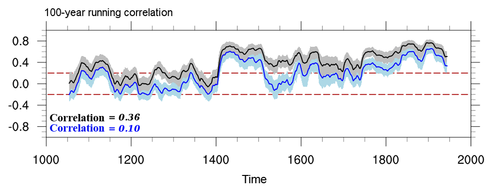
Figure 7100-year running correlation between BSL and ESL (black) and between BSL and median-reduced ESL (blue) with shading marking the uncertainty of the correlation using bootstrapping. Time series have been smoothed with an 11-year moving window prior to calculating the running correlations. Dashed red lines mark significant correlation on the 95th percentile confidence level. The long-term correlation is given in the bottom left corner.
Are the temporal modulations of coherent behavior between ESL and BSL due to different modes of variability and are there any systematic variations in ESLs? Spectral analysis (Fig. 8a) shows that ESLs exhibit white power spectra across all resolved periods (p=0.57 in Ljung–Box Q test) and do not – except for a minor spectral peak around 8 years – show preferred modes of variability (Fig. 8a). There is no significant difference between sites located along the coast of Lower Saxony and on sites at the coast of Schleswig-Holstein (not shown). On the other hand, BSL in terms of annual median sea level (Fig. 8b, separately shown for both winter and summer seasons) exhibits a red spectrum with more power on multidecadal and centennial timescales. The predominance of lower frequencies in the power spectrum stresses the influence of the ocean which carries the “memory” of the system. In summer and further off the coast (not shown), the high-frequency variability is reduced and thus lower frequencies are dominating the power spectrum. In winter, the higher frequencies are not as damped and the spectrum appears flatter as the wind stress effect on the water surface is more pronounced during winter when winds are strongest. Coherent variability of BSL and ESL is only visible on multidecadal timescales; at higher frequencies the random ESL variations outweigh the BSL ones and thus do not result in coherent variations for periods shorter than several decades (Fig. S7).
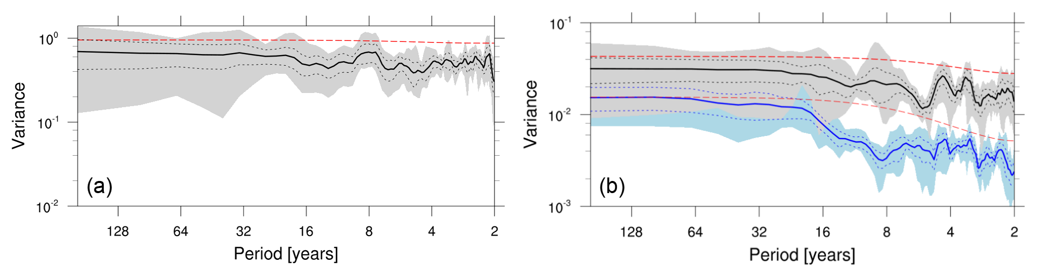
Figure 8Power spectrum of sea level at Cuxhaven: annual maximum sea level (a) and annual median sea level (b) split into winter (black) and summer season (blue). Spectra have been smoothed over 7 spectral estimates using a Daniell window (Daniell, 1946). The thick lines correspond to an average over nine overlapping 200-year subsets of the full time series, the shadings mark their range. Red lines indicate the 95 % confidence bounds using a theoretical Markov spectrum (red noise) and dashed black lines the 95 % confidence bounds derived from the nine realizations.
3.3 Relation to climate variability
Several mechanisms have been related to sea level variations, which mainly focused on those of the mean state. These range from large-scale atmospheric circulation patterns (e.g., Wakelin et al., 2003; Woodworth and Blackman, 2004; Chafik et al., 2017), over alongshore winds and resulting Kelvin waves (Sturges and Douglas, 2011; Calafat et al., 2012), to steric variations due to temperature oscillations (Frankcombe and Dijkstra, 2009). Mechanisms leading to longer-term ESL variations, however, remain more uncertain as data is limited, which challenges the robustness of statistical relationships between sea level extremes and other variables in the climate system. Yet, the patterns of large-scale climate variability over the North Atlantic that potentially influence ESLs may be different to those responsible for BSL variations. In order to investigate large-scale climate patterns associated with enhanced storm surge activity, we relate such periods with multidecadal climate variability, both internally generated as well as externally forced.
3.3.1 Internal variability
The NAO has often been linked to BSL variations in the North Sea (e.g., Wakelin et al., 2003; Woodworth and Blackman, 2004; Dangendorf et al., 2012), both through baroclinic as well as barotropic processes (Chen et al., 2014). When correlating observed ESLs from tide gauges with climate reanalysis data, some authors found the same large-scale patterns responsible for high ESLs as the pattern persists after removing the annual median (e.g., Woodworth et al., 2007; Marcos and Woodworth, 2017). Yet, the standard NAO is not necessarily the most indicative index: Kolker and Hameed (2007) have shown that the location of the centers of action comprising the NAO is affecting observed mean sea level trends and variability. Introducing a “tailored NAO index”, Dangendorf et al. (2014c) showed that slightly different pressure constellations than the standard NAO can better describe the observed ESL variability in the German Bight. Additionally, other teleconnection patterns such as the East Atlantic Pattern (EAP) or the Scandinavian pattern (SCA) have been shown to exert some influence on North Sea storminess (Seierstad et al., 2007) and mean sea level (Chafik et al., 2017). However, as some of the modes of climate variability are operating on similar timescales as the high-resolution instrumental sea level record, it is difficult to obtain robust conclusions.
As an indicator of the large-scale circulation, we compute positive composite maps of winter (October–March) mean sea level pressure (SLP) during times of high sea level at Cuxhaven, both in terms of ESL and, for comparison, BSL. Composites have been calculated as the average over periods where the simulated sea level time series at Cuxhaven exceeds its mean μ plus 1.5 times its standard deviation σ. The choice of the threshold is arbitrary, but the character of the pattern remains robust to minor changes in its value, specifically the range of ±0.25σ around the chosen threshold, especially for the BSL case. In the case of the ESL composites, the spatial variability of associated SLP patterns is large and single years can differ in shape and magnitude. The broader spatial character of the averaged anomaly pattern, however, is less affected. Again, we restrict the analysis to the extended winter season as storm surges primarily occur during these months. Furthermore, SLP has been low-pass filtered with a 3-year moving average to better investigate variability on longer timescales but to still be able to account for the slightly pronounced variations with periods of around 8 years.
The SLP pattern associated with enhanced BSL (Fig. 9a) deviates from the long-term winter mean pattern as the meridional pressure gradient over the North Atlantic is strengthened, comprising a negative SLP anomaly east of Iceland and a positive one over the Iberian Peninsula. This dipole with a meridional axis is similar to a positive NAO. The resulting correlation coefficients between (i) associated SLP index and NAO and (ii) the BSL time series and the NAO, computed as the leading principal component of the North Atlantic SLP, are significant (r=0.9 and 0.5, respectively), marking a qualitative agreement with the literature outlined above.
The SLP constellation favoring high ESL (Fig. 9b), however, differs slightly. As for BSL, it comprises a dipole over the northeast Atlantic, yet its centers of action are shifted to northeastern Scandinavia and the Gulf of Biscay, leading to a further eastward-stretching Icelandic Low and a clockwise-turned dipole favoring a more northwesterly wind component. This pattern is different from the meridional NAO-like dipole as in the case of elevated BSL. Due to the large ESL variability and the considerable noise in the extreme value time series, the composite pattern is pronounced weaker than the one associated with high BSL and exhibits a higher variance. Yet, despite this large spatial variance, there is an overall tendency towards a more zonal axis of the associated SLP anomaly pattern. Note that the SLP composites are averaged over the winter season while the ESL time series is based on winter maximum values; the SLP pattern, therefore, does not represent the situation during individual extreme storm floods but rather reflects a general circulation pattern during times of enhanced storm surge activity. The anomaly structure resembles the dipole described by Dangendorf et al. (2014b) for cross-correlations of SLP with observations of daily wind surges at Cuxhaven and agrees well with the mean weather situation triggering strong storm surges found by Heyen et al. (1996) in the wider region using statistical downscaling. Its spatial structure points to an influence of the Scandinavian Pattern in its negative phase (SCA−) onto the NAO centers of action, such as described by Chafik et al. (2017) for North Sea sea level variability. The pattern is also in agreement with a complementary analysis performed on the 2–6 d band-pass-filtered pressure variance (not shown), which indicates enhanced storm-track activity over the northeast Atlantic and North Sea.
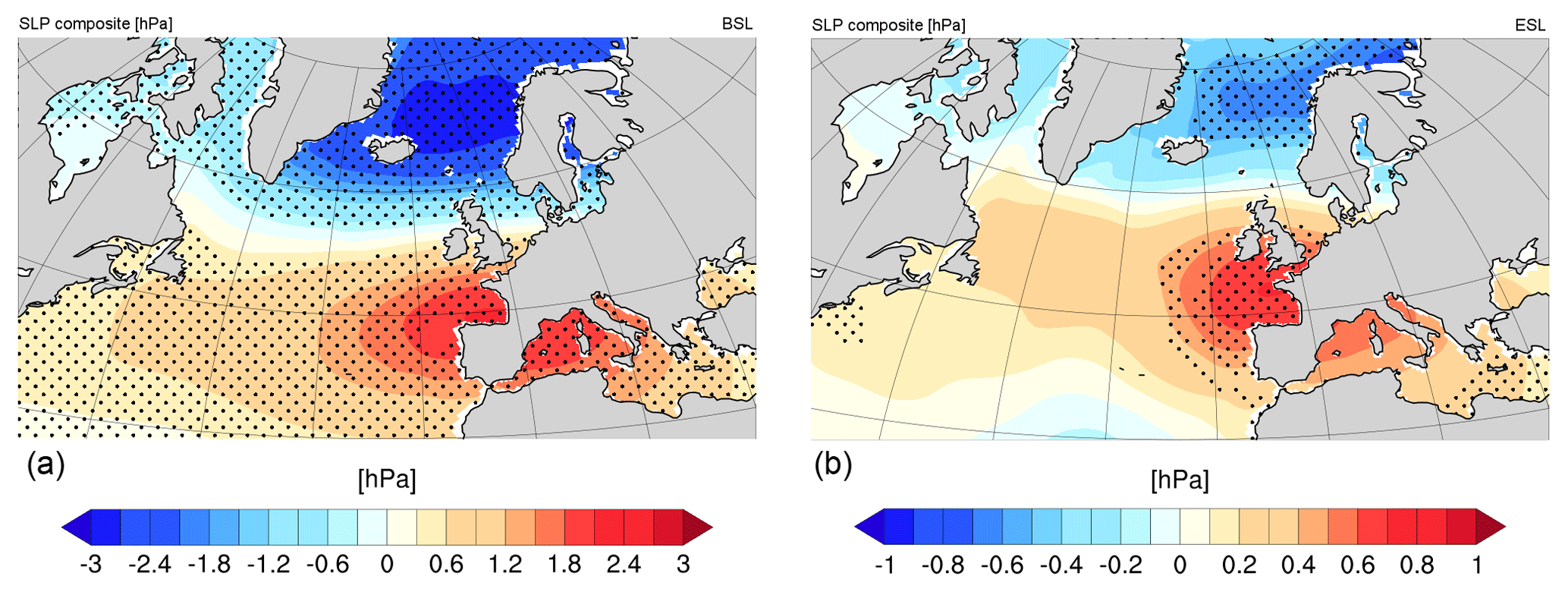
Figure 9Composite gridded winter SLP anomaly for periods of high BSL (a) and ESL (b) at Cuxhaven. Stippling marks areas significant at the 5 % confidence level.
As the SLP pattern associated with enhanced storm surge activity at Cuxhaven differs from the NAO, we use the shifted centers of action (Biscay – Northeast Scandinavia) to define a SLP index based on the normalized SLP difference between those points of the dipole to directly investigate the influence of this circulation pattern on storm surge activity in the wider region. Compared to the pattern associated with high BSL (correlation with NAO of r=0.9), this SLP pattern has a lower correlation with the NAO (r=0.67). As a result, the ESL time series at Cuxhaven also shows a weaker correlation with the NAO (r=0.19) than with the newly defined SLP pattern (r=0.31). Only towards the end of the millennium, BSL- and ESL-related SLP patterns evolve rather coherently. This feature may also explain why ESL and BSL show a higher coherency (see Fig. 7) during the last centuries. Regressing the time series of this SLP index onto the ESL field shows highest values not only in the German Bight (Fig. 10a), but also in the southern Baltic Sea where the regressed annual maximum sea levels are of similar magnitude. This suggests that periods of enhanced ESL activity in both the German Bight as well as the southern Baltic Sea are linked via the same large-scale circulation pattern. The spatial coherence of long-term ESL variations (see also Fig. S6) is in agreement with the study by Marcos et al. (2015) using data from tide gauges globally. The wavelet coherence – which can illustrate both timescales and timing of coherent behavior of both data series – between this index and ESLs at Cuxhaven shows that this relationship acts mainly on multidecadal to centennial timescales (Fig. 10b).
Figure 10(a) Pointwise regression of the SLP index derived from Fig. 9 onto annual maximum sea level (color shading, meters per unit of SLP index). (b) Wavelet coherence and cospectrum between annual maximum sea level at Cuxhaven and the tailored SLP index. Arrows to the right (left) indicate a positive (negative) correlation and upward (downward) arrows indicate a lag (lead) of ESL at Cuxhaven. Thick contours designate the 5 % significance level against red noise; the cone of influence is shown in a lighter shade.
The second downscaling (1500–2000) of the same GCM simulation yields a similar spatiotemporal variability. This indicates that the large-scale pattern responsible for high ESL activity is also a feature of the parent global simulation, which determines the temporal ESL variability on larger scales; the regionalization, however, can give added value in the development of dynamic systems such as atmospheric blocking and is more important for the specific surge heights and finer regional differences that are related to the exact wind direction and strength.
3.3.2 External forcing
It has been suggested that external influence, such as solar variations or large volcanic eruptions, can have an impact on magnitude and phasing of various climate phenomena such as the Atlantic Multidecadal Oscillation (AMO) (Otterå et al., 2010; Knudsen et al., 2014), longer-term anomalous temperature regimes (e.g., Miller et al., 2012), or atmospheric variability patterns such as the NAO (Swingedouw et al., 2011; Zanchettin et al., 2013), and can even trigger periods of enhanced storminess and coastal flooding (Barriopedro et al., 2010; Kaniewski et al., 2016; Martínez-Asensio et al., 2016). For instance, using geological proxy data of the central Mediterranean Sea, Kaniewski et al. (2016) argue for long-term correlations on cycles of around 2200 years and 230 years between storminess and solar activity; periods of lower solar activity will intensify the risk of frequent flooding in coastal areas. For the same region, Barriopedro et al. (2010) and Martínez-Asensio et al. (2016) also found coherent decadal changes in solar activity and autumn sea level extremes from tide gauges linked to the 11-year solar cycle through modulation of the atmospheric variability, namely a large-scale wave train pattern, implying an indirect role of solar activity in the decadal modulation of storm flood frequency.
The last millennium has seen substantial variations in solar irradiation, which have affected surface temperatures and lead to various longer-term temperature regimes such as the Late Maunder Minimum (1675–1710) or Dalton Minimum (1790–1840). Additionally, volcanic eruptions can alter the radiation balance substantially for a shorter time and clearly outweigh the variations of solar irradiance alone (see Fig. S3). Due to the different timescales, magnitude, and expected lag of a potential response to these external variations, it can be useful to separately investigate both forcings and their potential relationship with ESL variations through atmospheric variability.
However, a relation to extreme storm surge activity in the German Bight is not evident in our simulations. Wavelet coherence between total solar irradiance and ESL at Cuxhaven (Fig. S8a) and a “superposed epoch” analysis between volcanic eruptions and ESL (Fig. S8b) do not show a consistent significant relationship. Furthermore, the different temporal variations of ESL found in the downscalings of the two different global Last Millennium simulations (Fig. S4) stresses the dominance of natural variability in the timing of ESL variations. Due to the high internal variability of ESL, any signal from a potential external influence is masked and there is no evidence of coherent variability between German Bight storm surge activity and insolation variations – with or without the inclusion of volcanic forcing – during the last millennium. That is, extreme storm floods have occurred independently of major changes in forcing mechanisms or resulting long-term anomalous temperature regimes. This is in agreement with the findings by Fischer-Bruns et al. (2005) for multi-century simulations of midlatitude storms. The abovementioned link to atmospheric modes rather stresses the internal component of storm flood variability; this is in accordance with Gómez-Navarro and Zorita (2013), who have shown that the decadal variability of atmospheric modes such as the wintertime NAO is mainly unforced in CMIP5 Last Millennium simulations.
3.4 Relation to ESL components
Which components are governing ESL variability? As described above, the high-end extreme sea levels arise as a combination of three components: the tide, longer-term base level variations, and the surge residual, comprising all faster meteorological and oceanographic influences from both local as well as remote forcing. Following Woodworth and Blackman (2004), we investigate the surge residual via removal of the two other components, namely tide and background state in terms of the winter median. Removal of tides (using MATLAB program “t-tide”; Pawlowicz et al., 2002) alters the extreme storm surge time series by up to 1 m, depending on the tidal phase during the storm surge. Yet, after removal of tides and median, the general features of variability and spectra remains similar (not shown), stressing that the variability of extreme storm surges mainly stems from the atmosphere. This may not be surprising, as wind stress is expected to be the most important factor in shallow seas. The unchanged variability also implies that the absolute ESL index using annual maxima is a reasonable indicator of storm flood variability. Furthermore, the large-scale circulation pattern associated with high ESL qualitatively persists if the annual median is subtracted, although weaker. The comparably large spatial variance in the ESL pattern, however, leads to slight shifts in the location of the centers of action of the corresponding SLP dipole; yet, both ESL and ESL–BSL share a tendency towards a more zonal character of the associated SLP patterns. This similarity emphasizes that the SLP pattern associated with high ESL is linked to the surge residual variations. BSL variations are of much smaller amplitude than ESL variations and thus become marginal amid the strong variability of the latter. This is in accordance with findings by Woodworth and Blackman (2004) and Marcos and Woodworth (2017), who concluded that relationships with larger-scale climate variability, and specifically the NAO, remain even after removal of the other storm surge components.
The pronounced ESL variability on various timescales found in our simulation has important implications for the interpretation of the instrumental record, including trends as well as estimates of present and future storm floods. With a single realization of limited length, such as the instrumental ESL record, statements about potential correlation with BSL, climate variability, or alleged trends are statistically problematic and should therefore be treated with caution. For instance, setting recent ESL trends from the observational record (5.7±4.3 cm decade−1 for the 99.9th percentile of hourly sea level at Cuxhaven from 1953 to 2008; see Mudersbach et al., 2013) into context with the simulated ESL variability shows that the trends lie within the internal variability obtained from the long-term simulation: using a running trend with a window length similar to the aforementioned observational data (55 years) over the 1000 years of simulated data, a trend of the same or higher magnitude occurs in roughly 10 % of the segments. A trend higher than the given upper uncertainty limit (10 cm decade−1) still occurs 10 times during the 1000 years, or in around 1 % of the segments.
Furthermore, the large variations in high return values (around 1 m for RL100) illustrate the problem of using the standard approach of estimating extreme sea levels for flood protection standards. Typically, such estimates are based on parametric extreme value theory which is based on only a couple of decades of data (typically 30–50 years), be it the observational record or simulated data at the end of the century. The effect of fitting different extreme value distributions onto the same baseline period alone can be significant: a recent study by Wahl et al. (2017) quantified the uncertainties related to different extreme value estimates and showed that the “high-impact-low-probability” sea level states can vary substantially depending on both extreme value distribution and sampling technique. If, for example, a GEV distribution is fitted to a sample with more weight on more moderate extremes it might lead to a mismatch in higher return levels. For instance, Arns et al. (2013) have shown that for Cuxhaven, the use of r-largest order statistics with r>1 values per year leads to an overestimation of return water levels.
Together with the considerable spread of high-impact return level statistics, however, this results in even larger uncertainties: the error bars in Fig. 5 illustrate the uncertainties related to extrapolation from shorter subsets. The 1000-year return level (RL1000) estimated from the 100-year-long instrumental record yields error bars of 0.8 (3.2) m for a Gumbel (GEV) fit using maximum-likelihood estimation. The uncertainty is further stressed by the ensemble of ten 100-year-long segments, which in itself scatter around 1.2 m for 100-year return levels. This means in turn that a flood protection standard based on the highest observed sea level from a 100-year data set could as well correspond to a 30-year return level, only if another 100-year period were considered. That is, the observational record is not necessarily representative of the distribution and likelihood of the uppermost ESLs. The spread of the simulated RL100 from the 10 subsets is around twice as large as the 95 % confidence interval of the estimated RL1000 using a Gumbel distribution fit onto the observed 100-year data (green bar). This uncertainty range of the Gumbel fit doubles though if the spread in RL100 is taken into account (grey bar). The nonparametrically obtained RL1000 lies with 3.7 m within both distribution ranges, but closer to the median of the Gumbel distribution fits. Considering the large variations and corresponding uncertainties it is obvious that high-impact return levels (or flood protection standards for that matter) cannot reliably be inferred from short time series. The sample size considered as a base for parametric extreme value analysis affects not only the likely range of high-impact return events, but may also lead to a problematic negligence of potential scenarios.
How the data record combined with the choice of extreme value distribution impacts the estimation of high-impact return levels illustrated in Fig. 11. For this, we fit the GEV distribution and its special case of a Gumbel distribution to shorter subsets (33×30 and 16×60 year segments, respectively) of the full 1000 annual maximum sea levels and compare the RL100 estimates to the nonparametrically obtained RL100 (Fig. 11). A doubling of the data length from 30 to 60 years, for instance, roughly reduces the range of the RL100 from each segment's distribution fit to half and the uncertainty range to 1∕3 (GEV fit) or 2∕3 (Gumbel fit), respectively. The flexible GEV distribution gives more weight to the strongly varying tails of the distribution and results in a larger range of estimated RL100, which is mostly due to the variations in the shape parameter k, which strongly depends on the respective subset. If k is held constant (which is often assumed in nonstationary extreme value analysis; e.g. in Mudersbach and Jensen, 2010), the uncertainty range reduces considerably. In contrast, the Gumbel fit with a constant zero shape parameter leads to a narrower estimate of RL100. Yet, both distribution fits tend to favor the lower end of simulated 100-year return levels, although the RL100 inferred nonparametrically from the full simulation (green bar) lies within the interquartile range of both distribution estimates. This discrepancy can also manifest itself in the temporal variations: the parametric return value estimates can further exhibit different temporal behavior in comparison to the nonparametric plotting positions of the full simulation, and may even lie outside the associated uncertainty range. That is, even such a nonstationary extreme value analysis (e.g. Méndez et al., 2007; Mudersbach and Jensen, 2010) does not necessarily reflect the real variations in high return levels.
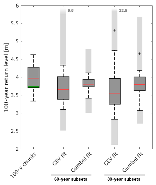
Figure 11Box-and-whisker plots of RL100 nonparametrically obtained from 10×100-year segments of the full simulation against RL100 estimates based on GEV and Gumbel distributions fitted to 60- and 30-year subsets using maximum likelihood. The range of the dashed whiskers represents the total range of the fits and light grey shading represents the maximum range of the 95 % confidence limits of the respective fits. The red lines indicate the median of the realizations, the green lines mark the RL100 directly inferred from the full 1000-year-long simulation.
Thus, existing ESL estimates based on limited data lengths do not reflect the full range of ESL variability, e.g. if data stem from a period of unusual state of a driving mechanism such as the SLP dipole outlined above.
Putting these findings into the context of climate change, mean sea level rise will – following a shift of the entire distribution – accordingly translate into a higher probability of occurrence of a particular level and lower return periods. However, while the probability distribution shifts to the right, the large noise level in the simulated ESL time series and the low explained variance by BSL imply that in the short term, German Bight ESLs might in reality show a much stronger or even a reversed trend.
Yet, in addition to a simple shift, a change in the shape of the distribution with increasing atmospheric GHG concentrations can further complicate the picture. Such a change may arise from changes in storm surge climate (e.g. due to an intensification and poleward shift of storm activity; e.g., Yin, 2005; Fischer-Bruns et al., 2005), or from a damping effect on the wind surge in a deeper sea; although this effect has been found to be comparably small (Lowe et al., 2001). This uncertainty in future storm surge projections is expressed by different findings in existing studies that show a spectrum from no (e.g., Sterl et al., 2009), over little (e.g., Langenberg et al., 1999; Woth, 2005), to considerable change (Lowe and Gregory, 2005). As the variations in ESL are of 1 order of magnitude higher than the corresponding BSL ones (see Fig.3), the variance explained by the latter is low and the detection of changes in the distribution difficult from a statistical point of view. With the strong, but random, fluctuations of ESL on timescales of years to decades, we expect existing estimates of ESL changes to be dominated by natural variability rather than climate change signals. Large ensemble simulations will be necessary to detect any significant change in ESL statistics in the presence of the high natural variability found in our simulation. Sterl et al. (2009) have already addressed this issue by using a large ensemble (17 members) of climate change scenario run with a regional storm surge model and found no signal from climate change on RL10 000 along the Dutch coast. Yet, most studies evaluating future storm risks on data shorter than the estimated return periods, either from observations or from scenario simulations, do not account for such large ensembles and thus systematically disregard ESL variability on timescales longer than the baseline periods. The ESL variation can be substantial, as the large spread of simulated upper-end return levels during the last millennium has shown. For instance, assuming a sea level rise of 0.5 m until the end of the century and given the quantified ESL variability, more than roughly 200 (350) years of data would be necessary for RL100 estimates (95 % confidence bounds) using a Gumbel fit to range over less than the estimated signal. Without using large ensembles, ESL projections may be biased by the respective baseline period for extreme value analysis; and even worse, with a small ensemble size or one realization only (e.g. the instrumental record) we cannot say whether they are biased or not. On the other hand, the high internal variability which is essentially irreducible (Fischer et al., 2013) also implies that even perfect models cannot provide well-constrained information on local ESL changes from one realization that might be desirable for adaptation planners.
A couple of caveats that may have an influence on our results are worth discussing. Simulated ESLs are – relative to the long-term mean – biased low, which is most likely related to an underrepresentation of the tidal range in the German Bight (see Fig. S1) and to simplifications in the model bathymetry: the ocean model's uppermost layer thickness of 16 m exceeds the real depth of the shallow waters in many coastal areas of the German Bight and thus may lead to lower wind surges than observed. At Cuxhaven, this effect should be smaller than at points along the flatter Wadden Sea where the tidal oscillations and the shallow waters lead to coastline changes which cannot be represented here. The influence of the bottom topography is expected to play a subordinate role compared to the rather complex horizontal coastline geometry. Yet, in terms relative to mean high waters, simulated ESL statistics agree well with observations, and the temporal variability is not affected by this.
Additionally, the model does not allow for changes in bathymetry, shoreline, or coastal management that may influence relative sea levels. This may benefit the homogeneity of the simulated sea level variations but may hamper the comparability to observations. Processes such as changes in local bathymetry, wave interference at ports, or simply inconsistencies in the data record can obstruct the homogeneity of observations from tide gauge records. Additionally, discrepancies between the exact tide gauge position and the nearest-neighbor grid box can further complicate the picture. A direct comparison between simulated and observed sea levels should therefore be treated with caution. Furthermore, a transient sea level rise due to melting of ice sheets, postglacial isostatic rebound, or the thermosteric effect is not accounted for in the model and a potential increase in ESL with a gradual rise in the BSL base could not be investigated. Such transient sea level changes can further impact ESLs on longer timescales, since the sea level distribution shifts with changes in BSL and may potentially also change in shape.
Finally, the results were obtained by downscaling simulations from one GCM only. Potential biases in the parent GCM can thus feed into the downscaled results. For instance, both northern hemispheric storm tracks as well as the North Atlantic Current have been found to be too zonal in ECHAM and MPIOM, respectively (Sidorenko et al., 2015; Jungclaus et al., 2013).
As the downscaling of another ensemble member of the parent GCM simulations has shown, the temporal ESL variations of the two different downscalings differ significantly (see Fig. S4), albeit their long-term statistics are comparable. That is, any external influence on long-term ESL variability is negligible and it is the natural variability of the parent GCM which determines the temporal variability on a larger scale. The regionalization, however, can offer more detailed dynamical patterns such as atmospheric blocking. With more precise wind speeds and directions as well as the consideration of regional shelf dynamics, it is thus more important for individual surge heights and finer regional differences. The variability due to the downscaling has been addressed by performing an additional downscaling of the same global simulation which has yielded similar spatiotemporal variability (see Fig. S5), indicating that the temporal ESL variability directly linked to the downscaling is negligible. This is in accordance with Woth et al. (2006), who, comparing a number of regional climate models, concluded that the added uncertainty from the downscaling step of ESL variations from global to regional models was comparably small.
Our study has provided the first coupled downscaling simulation focusing on storm surges and sea level evolution, which gives an unprecedentedly long high-resolution data record that can extend the knowledge of long-term ESL variability based on observations from tide gauge data which are limited in time and space. This simulation renders nonparametric extreme value analysis possible and has the advantage of not relying on extreme value distributions that are typically applied to short data series to provide information about return periods longer than the original time series, as well as their associated uncertainties. The special setup of coupling a high-resolution regional atmospheric model to a global ocean model including tides combines their respective advantages of (i) a consistent simulation of signals both inside and outside the region of interest and (ii) a sufficiently high resolution in the region of interest to properly account for regional ocean–atmosphere dynamics and other shelf processes. At the same time, the continuous global simulation allows for setting the ESL variability into the context of simulated climate states.
The variability of extreme storm floods has been investigated through the means of annual maximum sea levels at Cuxhaven; the results obtained from different extreme value indices and other grid points along the German Bight coastline, however, do not differ significantly, suggesting that the qualitative behavior and variability are robust and do not depend on the extreme value sampling method or exact location.
Our results suggest the following.
-
The model reproduces observed storm surge statistics at Cuxhaven both in terms of seasonality as well as magnitude above mean high waters.
-
ESL variations are large but operate on a white spectrum and do not exhibit significant oscillatory modes beyond the seasonal cycle.
-
High-impact extreme events vary substantially on timescales longer than the typically available base period for return period estimates. Estimates of ESL obtained via the standard parametric approach based on short data records are therefore not representative for the full ESL variations.
-
Long-term ESL variations in the German Bight are regionally consistent, indicating a common large-scale forcing. Large-scale circulation regimes that favor periods of enhanced ESL in the German Bight are similar to those associated with elevated BSL, but the location of the respective centers of action of the governing SLP dipole differs. While BSL variations correlate well with the wintertime NAO, ESL variations are rather associated with a shifted pressure pattern like NAO+ or SCA−, leading to a stronger local northwesterly wind component.
-
Any potential links to BSL fluctuations as well as external influence through solar variability or volcanic activity are masked by the strong internal variability of ESL. This is in accordance with the findings by Fischer-Bruns et al. (2005), who, using coupled Last Millennium simulations of the last five centuries, concluded that the natural variability of midlatitude storms is not related to solar, volcanic, or GHG forcing nor to anomalous climate states such as the Maunder Minimum. Similar conclusions have been made for North Atlantic summer storm tracks over Europe by combining observations, simulations, and reconstructions of the last millennium (Gagen et al., 2016).
We thus conclude that the magnitude of ESL and existing estimates of changes are dominated by natural variability rather than forced signals. Given the large variability from our simulation, large ensemble simulations are required to detect a potential future change in ESL statistics with respect to climate-change-induced BSL.
Nevertheless, the obtained information on the statistics of ESL variability together with the established links to large-scale climate variability may be used to better explore future pathways of extreme sea levels. Owing to the large ESL variability, a responsible adaptation strategy should therefore reflect the range of possible developments rather than solely being designed to a forced signal. At the end, uncertainties in both sea level rise projections as well as ESL estimates need to be better understood and combined to fully assess potential impacts and required adaptation measures.
Primary data and scripts used in the analysis that may be useful in reproducing the work are archived by the Max Planck Institute for Meteorology and can be obtained by contacting publications@mpimet.mpg.de.
The supplement related to this article is available online at: https://doi.org/10.5194/os-15-651-2019-supplement.
UM came up with the idea for the paper and developed the model code. AL and UM jointly designed the experiments; simulation and analysis were carried out by AL. The paper was written by AL with contributions from UM.
The authors declare that they have no conflict of interest.
The research was supported by the Max Planck Society and by the German Research Foundation (DFG) funded project SEASTORM under the umbrella of the Priority Programme SPP-1889 “Regional Sea Level Change and Society” (grant no. MI 603/5-1). The authors acknowledge Eduardo Moreno-Chamorro and Johann Jungclaus for producing the past1000 global simulations and Sönke Dangendorf and Wilfried Wiechmann for providing the observational data from selected tide gauges. We thank Johann Jungclaus and Moritz Mathis, as well as editor Markus Meier and three anonymous reviewers, for their constructive comments and remarks which helped to improve this paper. We further acknowledge the German Climate Computing Center (DKRZ) for providing the necessary computational resources.
This research has been supported by the German Research Foundation (DFG) (grant no. MI 603/5-1).
The article processing charges for this open-access
publication were covered by the Max Planck Society.
This paper was edited by Markus Meier and reviewed by three anonymous referees.
Araújo, I. B. and Pugh, D. T.: Sea levels at Newlyn 1915–2005: analysis of trends for future flooding risks, J. Coast. Res., 24, 203–212, 2008. a
Arns, A., Wahl, T., Haigh, I., Jensen, J., and Pattiaratchi, C.: Estimating extreme water level probabilities: A comparison of the direct methods and recommendations for best practise, Coast. Engin., 81, 51–66, 2013. a
Barriopedro, D., García-Herrera, R., Lionello, P., and Pino, C.: A discussion of the links between solar variability and high-storm-surge events in Venice, J. Geophys. Res.-Atmos., 115, D13101, https://doi.org/10.1029/2009JD013114, 2010. a, b
Calafat, F., Chambers, D., and Tsimplis, M.: Mechanisms of decadal sea level variability in the eastern North Atlantic and the Mediterranean Sea, J. Geophys. Res.-Ocean., 117, C09022, https://doi.org/10.1029/2012JC008285, 2012. a, b
Chafik, L., Nilsen, J. E. Ø., and Dangendorf, S.: Impact of North Atlantic teleconnection patterns on Northern European sea level, J. Mar. Sci. Eng., 5, 43, 32 pp., 2017. a, b, c
Chen, X., Dangendorf, S., Narayan, N., O'Driscoll, K., Tsimplis, M. N., Su, J., Mayer, B., and Pohlmann, T.: On sea level change in the North Sea influenced by the North Atlantic Oscillation: local and remote steric effects, Estuarine, Coas. Shelf Sci., 151, 186–195, 2014. a, b
Coles, S., Bawa, J., Trenner, L., and Dorazio, P.: An introduction to statistical modeling of extreme values, Springer, Vol. 208, 208 pp., 2001. a, b
Crowley, T. J., Zielinski, G., Vinther, B., Udisti, R., Kreutz, K., Cole-Dai, J., and Castellano, E.: Volcanism and the little ice age, PAGES news, 16, 22–23, 2008. a
Dangendorf, S., Wahl, T., Hein, H., Jensen, J., Mai, S., and Mudersbach, C.: Mean sea level variability and influence of the North Atlantic Oscillation on long-term trends in the German Bight, Water, 4, 170–195, 2012. a, b
Dangendorf, S., Mudersbach, C., Jensen, J., Anette, G., and Heinrich, H.: Seasonal to decadal forcing of high water level percentiles in the German Bight throughout the last century, Ocean Dynam., 63, 533–548, 2013a. a
Dangendorf, S., Mudersbach, C., Wahl, T., and Jensen, J.: Characteristics of intra-, inter-annual and decadal sea-level variability and the role of meteorological forcing: the long record of Cuxhaven, Ocean Dynam., 63, 209–224, 2013b. a
Dangendorf, S., Calafat, F. M., Arns, A., Wahl, T., Haigh, I. D., and Jensen, J.: Mean sea level variability in the North Sea: Processes and implications, J. Geophys. Res.-Ocean., 119, 6820–6841, https://doi.org/10.1002/2014JC009901, 2014a. a
Dangendorf, S., Müller-Navarra, S., Jensen, J., Schenk, F., Wahl, T., and Weisse, R.: North Sea storminess from a novel storm surge record since AD 1843, J. Clim., 27, 3582–3595, 2014b. a, b
Dangendorf, S., Wahl, T., Nilson, E., Klein, B., and Jensen, J.: A new atmospheric proxy for sea level variability in the southeastern North Sea: observations and future ensemble projections, Clim. Dynam., 43, 447–467, 2014c. a, b
Daniell, P.: Discussion on Symposium on autocorrelation in time series, J. Roy. Stat. Soc., 8, 88–90, 1946. a
Donat, M. G., Leckebusch, G. C., Pinto, J. G., and Ulbrich, U.: Examination of wind storms over Central Europe with respect to circulation weather types and NAO phases, Int. J. Climatol., 30, 1289–1300, 2010. a
Elizalde, A., Gröger, M., Mathis, M., MIkOLAJEw-ICZ, U., BüLOw, K., Hüttl-Kabus, S., Klein, B., and GANSkE, A.: MPIOM-REMO A Coupled Regional Model for the North Sea, KLIWAS-Schriftenreihe KLIWAS-58/2014, 10, 2014. a
Ezer, T., Haigh, I. D., and Woodworth, P. L.: Nonlinear sea-level trends and long-term variability on Western European Coasts, J. Coast. Res., 32, 744–755, 2015. a
Fischer, E. M., Beyerle, U., and Knutti, R.: Robust spatially aggregated projections of climate extremes, Nat. Clim. Change, 3, 1033, https://doi.org/10.1038/nclimate2051, 2013. a
Fischer-Bruns, I., von Storch, H., González-Rouco, J., and Zorita, E.: Modelling the variability of midlatitude storm activity on decadal to century time scales, Clim. Dynam., 25, 461–476, 2005. a, b, c
Frankcombe, L. and Dijkstra, H.: Coherent multidecadal variability in North Atlantic sea level, Geophys. Res. Lett., 36, L15604, 2009. a
Gagen, M. H., Zorita, E., McCarroll, D., Zahn, M., Young, G. H., and Robertson, I.: North Atlantic summer storm tracks over Europe dominated by internal variability over the past millennium, Nat. Geosci., 9, 630–635, 2016. a
Gerber, M., Ganske, A., Müller-Navarra, S., and Rosenhagen, G.: Categorisation of Meteorological Conditions for Storm Tide Episodes in the German Bight, Meteorologische Zeitschrift, 447–462, 2016. a
Giorgetta, M. A., Roeckner, E., Mauritsen, T., Stevens, B., Bader, J., Crueger, T., Esch, M., Rast, S., Kornblueh, L., Schmidt, H., Kinne, S., Möbis, B., and Krismer, T.: The atmospheric general circulation model ECHAM6, Model description, Max Planck Inst. for Meteorol., Hamburg, Germany, 2012. a
Gómez-Navarro, J. and Zorita, E.: Atmospheric annular modes in simulations over the past millennium: No long-term response to external forcing, Geophys. Res. Lett., 40, 3232–3236, 2013. a
Gönnert, G. and Sossidi, K.: A new approach to calculate extreme storm surges: analysing the interaction of storm surge components, WIT Trans. Ecol. Envir., 149, 139–150, 2011. a
Hadler, H., Vött, A., Newig, J., Emde, K., Finkler, C., Fischer, P., and Willershäuser, T.: Geoarchaeological evidence of marshland destruction in the area of Rungholt, present-day Wadden Sea around Hallig Südfall (North Frisia, Germany), by the Grote Mandrenke in 1362 AD, Quatern. Int., 473, 37–54, 2018. a
Heimreich, M. A. (Editor: Falck, N.: Nordfriesische Chronik, Tondern,Quaternary 1819. a
Heyen, H., Zorita, E., and von Storch, H.: Statistical downscaling of monthly mean North Atlantic air-pressure to sea level anomalies in the Baltic Sea, Tellus A, 48, 312–323, 1996. a
Horsburgh, K. and Wilson, C.: Tide-surge interaction and its role in the distribution of surge residuals in the North Sea, J. Geophys. Res.-Ocean., 112, C08003, https://doi.org/10.1029/2006JC004033, 2007. a
Hurrell, J. W.: Decadal trends in the North Atlantic Oscillation: Regional Temperatures and precipitation, Science, 269, 676–679, 1995. a
Jacob, D. and Podzun, R.: Sensitivity studies with the regional climate model REMO, Meteorol. Atmos. Phys., 63, 119–129, 1997. a
Jacob, D., Petersen, J., Eggert, B., Alias, A., Christensen, O. B., Bouwer, L. M., Braun, A., Colette, A., Déqué, M., Georgievski, G., Georgopoulou, E., Gobiet, A., Menut, L., Nikulin, G., Haensler, A., Hempelmann, N., Jones, C., Keuler, K., Kovats, S., Kröner, N., Kotlarski, S., Kriegsmann, A., Martin, E., van Meijgaard, E., Moseley, C., Pfeifer, S., Preuschmann, S., Radermacher, C., Radtke, K., Rechid, D., Rounsevell, M., Samuelsson, P., Somot, S., Soussana, J.-F., Teichmann, C., Valentini, R., Vautard, R., Weber, B., and Yiou, P.: EURO-CORDEX: new high-resolution climate change projections for European impact research, Reg. Environ. Change, 14, 563–578, 2014. a
Jensen, J., Frank, T., and Wahl, T.: Analyse von hochaufgelösten Tidewasserständen und Ermittlung des MSL an der deutschen Nordseeküste (AMSeL), Die Küste, 78, 59–163, 2011. a
Jungclaus, J., Fischer, N., Haak, H., Lohmann, K., Marotzke, J., Matei, D., Mikolajewicz, U., Notz, D., and Storch, J.: Characteristics of the ocean simulations in the Max Planck Institute Ocean Model (MPIOM) the ocean component of the MPI-Earth system model, J. Adv. Model. Earth Sy., 5, 422–446, 2013. a, b
Jungclaus, J. H., Lohmann, K., and Zanchettin, D.: Enhanced 20th-century heat transfer to the Arctic simulated in the context of climate variations over the last millennium, Clim. Past, 10, 2201–2213, https://doi.org/10.5194/cp-10-2201-2014, 2014. a, b
Kaniewski, D., Marriner, N., Morhange, C., Faivre, S., Otto, T., and Van Campo, E.: Solar pacing of storm surges, coastal flooding and agricultural losses in the Central Mediterranean, Sci. Rep., 6, 25197, https://doi.org/10.1038/srep25197, 2016. a, b
Kauker, F. and Langenberg, H.: Two models for the climate change related development of sea levels in the North Sea a comparison, Clim. Res., 15, 61–67, 2000. a, b
Kauker, F. and von Storch, H.: Regionalization of climate model results for the North Sea, externer Bericht der GKSS, GKSS 2000/28, 2000. a, b
Knudsen, M. F., Jacobsen, B. H., Seidenkrantz, M.-S., and Olsen, J.: Evidence for external forcing of the Atlantic Multidecadal Oscillation since termination of the Little Ice Age, Nat. Commun., 5, 3323, https://doi.org/10.1038/ncomms4323, 2014. a
Kolker, A. S. and Hameed, S.: Meteorologically driven trends in sea level rise, Geophys. Res. Lett., 34, L23616, https://doi.org/10.1029/2007GL031814, 2007. a
Langenberg, H., Pfizenmayer, A., von Storch, H., and Sündermann, J.: Storm-related sea level variations along the North Sea coast: natural variability and anthropogenic change, Cont. Shelf Res., 19, 821–842, 1999. a, b
Lowe, J. and Gregory, J.: The effects of climate change on storm surges around the United Kingdom, Philosophical Transactions of the Royal Society of London A: Mathematical, Phys. Engin. Sci., 363, 1313–1328, 2005. a
Lowe, J., Gregory, J. M., and Flather, R.: Changes in the occurrence of storm surges around the United Kingdom under a future climate scenario using a dynamic storm surge model driven by the Hadley Centre climate models, Clim. Dynam., 18, 179–188, 2001. a
Marcos, M. and Woodworth, P. L.: Spatiotemporal changes in extreme sea levels along the coasts of the North Atlantic and the Gulf of Mexico, J. Geophys. Res.-Ocean., 122, 7031–7048, 2017. a, b, c
Marcos, M., Tsimplis, M. N., and Shaw, A. G.: Sea level extremes in southern Europe, J. Geophys. Res.-Ocean., 114, C01007, https://doi.org/10.1029/2008JC004912, 2009. a, b, c
Marcos, M., Calafat, F. M., Berihuete, Á., and Dangendorf, S.: Long-term variations in global sea level extremes, J. Geophys. Res.-Ocean., 120, 8115–8134, 2015. a
Marsland, S. J., Bindoff, N., Williams, G., and Budd, W.: Modeling water mass formation in the Mertz Glacier Polynya and Adélie Depression, east Antarctica, J. Geophys. Res.-Ocean., 109, C11003, https://doi.org/10.1029/2004JC002441, 2004. a
Martínez-Asensio, A., Tsimplis, M. N., and Calafat, F. M.: Decadal variability of European sea level extremes in relation to the solar activity, Geophys. Res. Lett., 43, 11744-–11750, https://doi.org/10.1002/2016GL071355, 2016. a, b
Mathis, M., Elizalde, A., and Mikolajewicz, U.: Which complexity of regional climate system models is essential for downscaling anthropogenic climate change in the Northwest European Shelf?, Clim. Dynam., 50, 2637–2659, 2018. a
Mawdsley, R. J. and Haigh, I. D.: Spatial and temporal variability and long-term trends in skew surges globally, Front. Mar. Sci., 3, 29, 17 pp., 2016. a
Méndez, F. J., Menéndez, M., Luceño, A., and Losada, I. J.: Estimation of the long-term variability of extreme significant wave height using a time-dependent peak over threshold (pot) model, J. Geophys. Res.-Ocean., 111, C07024, https://doi.org/10.1029/2005JC003344, 2006. a
Méndez, F. J., Menéndez, M., Luceño, A., and Losada, I. J.: Analyzing monthly extreme sea levels with a time-dependent GEV model, J. Atmos. Ocean. Technol., 24, 894–911, 2007. a, b
Menéndez, M. and Woodworth, P. L.: Changes in extreme high water levels based on a quasi-global tide-gauge data set, J. Geophys. Res.-Ocean., 115, C10011, https://doi.org/10.1029/2009JC005997, 2010. a, b
Mikolajewicz, U., Sein, D. V., Jacob, D., Königk, T., Podzun, R., and Semmler, T.: Simulating Arctic sea ice variability with a coupled regional atmosphere-ocean-sea ice model, Meteorol. Z., 14, 793–800, 2005. a
Miller, G. H., Geirsdóttir, Á., Zhong, Y., Larsen, D. J., Otto-Bliesner, B. L., Holland, M. M., Bailey, D. A., Refsnider, K. A., Lehman, S. J., Southon, J. R., Anderson, C., Björnsson, H., and Thordarson, T.: Abrupt onset of the Little Ice Age triggered by volcanism and sustained by sea-ice/ocean feedbacks, Geophys. Res. Lett., 39, L02708, https://doi.org/10.1029/2011GL050168, 2012. a
Ministerium für ländliche Räume, Landesplanung, Landwirtschaft und Tourismus des Landes Schleswig-Holstein (Ed.): Generalplan Küstenschutz des Landes Schleswig-Holstein, Kiel, 2012. a, b
Moreno-Chamarro, E., Zanchettin, D., Lohmann, K., Luterbacher, J., and Jungclaus, J. H.: Winter amplification of the European Little Ice Age cooling by the subpolar gyre, Sci. Rep., 7, 9981, https://doi.org/10.1038/s41598-017-07969-0, 2017. a, b
Mudersbach, C. and Jensen, J.: Nonstationary extreme value analysis of annual maximum water levels for designing coastal structures on the German North Sea coastline, J. Flood Risk Manag., 3, 52–62, 2010. a, b
Mudersbach, C., Wahl, T., Haigh, I. D., and Jensen, J.: Trends in high sea levels of German North Sea gauges compared to regional mean sea level changes, Cont. Shelf Res., 65, 111–120, 2013. a, b, c, d, e, f
Müller-Navarra, S., Lange, W., Dick, S., and Soetje, K.: Über die Verfahren der Wasserstands-und Sturmflutvorhersage, Promet, 29, 117–124, 2003. a
Otterå, O. H., Bentsen, M., Drange, H., and Suo, L.: External forcing as a metronome for Atlantic multidecadal variability, Nat. Geosci., 3, 688–694, 2010. a
Pawlowicz, R., Beardsley, B., and Lentz, S.: Classical tidal harmonic analysis including error estimates in MATLAB using T_TIDE, Comput. Geosci., 28, 929–937, 2002. a
Plüß, A.: Nichtlineare Wechselwirkung der Tide auf Anderungen des Meeresspiegels im Küste/Astuar am Beispiel der Elbe, in: Klimaänderung und Küstenschutz, edited by: Gönnert, G., Grassl, H., Kellat, D., Kunz, H., Probst, B., von Storch, H., and Sündermann, J., 129–138, 2004. a
Pugh, D. and Woodworth, P.: Sea-level science: understanding tides, surges, tsunamis and mean sea-level changes, 407 pp., Cambridge Univ. Press, Cambridge, UK, 2014. a
Schmidt, G. A., Jungclaus, J. H., Ammann, C. M., Bard, E., Braconnot, P., Crowley, T. J., Delaygue, G., Joos, F., Krivova, N. A., Muscheler, R., Otto-Bliesner, B. L., Pongratz, J., Shindell, D. T., Solanki, S. K., Steinhilber, F., and Vieira, L. E. A.: Climate forcing reconstructions for use in PMIP simulations of the Last Millennium (v1.1), Geosci. Model Dev., 5, 185–191, https://doi.org/10.5194/gmd-5-185-2012, 2012. a
Seierstad, I., Stephenson, D., and Kvamstø, N.: How useful are teleconnection patterns for explaining variability in extratropical storminess?, Tellus A, 59, 170–181, 2007. a
Sein, D. V., Mikolajewicz, U., Gröger, M., Fast, I., Cabos, W., Pinto, J. G., Hagemann, S., Semmler, T., Izquierdo, A., and Jacob, D.: Regionally coupled atmosphere-ocean-sea ice-marine biogeochemistry model ROM: 1. Description and validation, J. Adv. Model. Earth Sy., 7, 268–304, 2015. a
Sidorenko, D., Rackow, T., Jung, T., Semmler, T., Barbi, D., Danilov, S., Dethloff, K., Dorn, W., Fieg, K., Gößling, H. F., Handorf, D., Harig, S., Hiller, W., Juricke, S., Losch, M., Schröter, J., Sein, D. V., and Wang, Q.: Towards multi-resolution global climate modeling with ECHAM6–FESOM. Part I: model formulation and mean climate, Clim. Dynam., 44, 757–780, 2015. a
Sterl, A., van den Brink, H., de Vries, H., Haarsma, R., and van Meijgaard, E.: An ensemble study of extreme storm surge related water levels in the North Sea in a changing climate, Ocean Sci., 5, 369–378, https://doi.org/10.5194/os-5-369-2009, 2009. a, b
Sturges, W. and Douglas, B. C.: Wind effects on estimates of sea level rise, J. Geophys. Res.-Ocean., 116, C06008, https://doi.org/10.1029/2010JC006492, 2011. a, b
Swingedouw, D., Terray, L., Cassou, C., Voldoire, A., Salas-Mélia, D., and Servonnat, J.: Natural forcing of climate during the last millennium: fingerprint of solar variability, Clim. Dynam., 36, 1349–1364, 2011. a
Taylor, K. E., Stouffer, R. J., and Meehl, G. A.: An overview of CMIP5 and the experiment design, Bull. Am. Meteor. Soc., 93, 485–498, 2012. a
Thomas, M., Sündermann, J., and Maier-Reimer, E.: Consideration of ocean tides in an OGCM and impacts on subseasonal to decadal polar motion excitation, Geophys. Res. Lett., 28, 2457–2460, 2001. a
Tsimplis, M. and Woodworth, P.: The global distribution of the seasonal sea level cycle calculated from coastal tide gauge data, J. Geophys. Res.-Ocean., 99, 16031–16039, 1994. a
Valcke, S.: The OASIS3 coupler: a European climate modelling community software, Geosci. Model Dev., 6, 373–388, https://doi.org/10.5194/gmd-6-373-2013, 2013. a
von Storch, H. and Reichardt, H.: A scenario of storm surge statistics for the German Bight at the expected time of doubled atmospheric carbon dioxide concentration, J. Clim., 10, 2653–2662, 1997. a
von Storch, H. and Woth, K.: Storm surges: perspectives and options, Sustainability Science, 3, 33–43, 2008. a
Wahl, T. and Chambers, D. P.: Evidence for multidecadal variability in US extreme sea level records, J. Geophys. Res.-Ocean., 120, 1527–1544, 2015. a
Wahl, T., Jensen, J., Frank, T., and Haigh, I. D.: Improved estimates of mean sea level changes in the German Bight over the last 166 years, Ocean Dynam., 61, 701–715, 2011. a
Wahl, T., Haigh, I. D., Nicholls, R. J., Arns, A., Dangendorf, S., Hinkel, J., and Slangen, A. B.: Understanding extreme sea levels for broad-scale coastal impact and adaptation analysis, Nat. Commun., 8, 16075, https://doi.org/10.1038/ncomms16075, 2017. a
Wakelin, S., Woodworth, P., Flather, R., and Williams, J.: Sea-level dependence on the NAO over the NW European Continental Shelf, Geophys. Res. Lett., 30, 1403, https://doi.org/10.1029/2003GL017041, 2003. a, b, c
Wang, Y.-M., Lean, J., and Sheeley Jr., N.: Modeling the Sun’s magnetic field and irradiance since 1713, Astrophys. J., 625, 522–538, 2005. a
WASA-group: Changing waves and storms in the Northeast Atlantic?, Bull. Am. Meteor. Soc., 79, 741–760, 1998. a, b
Weisse, R. and Plüß, A.: Storm-related sea level variations along the North Sea coast as simulated by a high-resolution model 1958–2002, Ocean Dynam., 56, 16–25, 2006. a, b, c
Weisse, R., von Storch, H., Niemeyer, H. D., and Knaack, H.: Changing North Sea storm surge climate: An increasing hazard?, Ocean Coast. Manag., 68, 58–68, 2012. a
Weisse, R., Bellafiore, D., Menéndez, M., Méndez, F., Nicholls, R. J., Umgiesser, G., and Willems, P.: Changing extreme sea levels along European coasts, Coast. Engin., 87, 4–14, 2014. a
Woodworth, P., Flather, R., Williams, J., Wakelin, S., and Jevrejeva, S.: The dependence of UK extreme sea levels and storm surges on the North Atlantic Oscillation, Cont. Shelf Res., 27, 935–946, 2007. a, b
Woodworth, P. L. and Blackman, D. L.: Evidence for systematic changes in extreme high waters since the mid-1970s, J. Clim., 17, 1190–1197, 2004. a, b, c, d, e, f, g, h
Woodworth, P. L., Menéndez, M., and Gehrels, W. R.: Evidence for century-timescale acceleration in mean sea levels and for recent changes in extreme sea levels, Surv. Geophys., 32, 603–618, 2011. a
Woth, K.: Regionalization of global climate change scenarios: An ensemble study of possible changes in the North Sea storm surge statistics, Ph.D. thesis, Universität Hamburg Hamburg, 2005. a, b
Woth, K., Weisse, R., and von Storch, H.: Climate change and North Sea storm surge extremes: an ensemble study of storm surge extremes expected in a changed climate projected by four different regional climate models, Ocean Dynam., 56, 3–15, 2006. a
Yin, J. H.: A consistent poleward shift of the storm tracks in simulations of 21st century climate, Geophys. Res. Lett., 32, L18701, https://doi.org/10.1029/2005GL023684, 2005. a
Zanchettin, D., Timmreck, C., Bothe, O., Lorenz, S. J., Hegerl, G., Graf, H.-F., Luterbacher, J., and Jungclaus, J. H.: Delayed winter warming: A robust decadal response to strong tropical volcanic eruptions?, Geophys. Res. Lett., 40, 204–209, 2013. a