2.1 Model description

We employed the Semi-implicit Cross-scale Hydroscience Integrated System Model (SCHISM; Zhang et al., 2015, 2016), an open-source community-supported modeling system derived from the early SELFE model (Zhang and Baptista, 2008). SCHISM uses a highly efficient semi-implicit finite-element and finite-volume method with a Eulerian–Lagrangian algorithm to solve the turbulence-averaged Navier–Stokes equations under the hydrostatic approximation. It uses the generic length-scale model of Umlauf and Burchard (2003) with the stability function of Kantha and Clayson (1994) for turbulence closure. One of the major advantages of the model is that it has the capability of employing a very flexible vertical grid system, robustly and faithfully resolving the complex topography in estuarine and oceanic systems without any smoothing (Zhang et al., 2016; Stanev et al., 2017; Du et al., 2018b; Ye et al., 2018). A more detailed description of the SCHISM, including the governing equations, horizontal and vertical grids, numerical solution methods, and boundary conditions, can be found in Zhang et al. (2015, 2016).

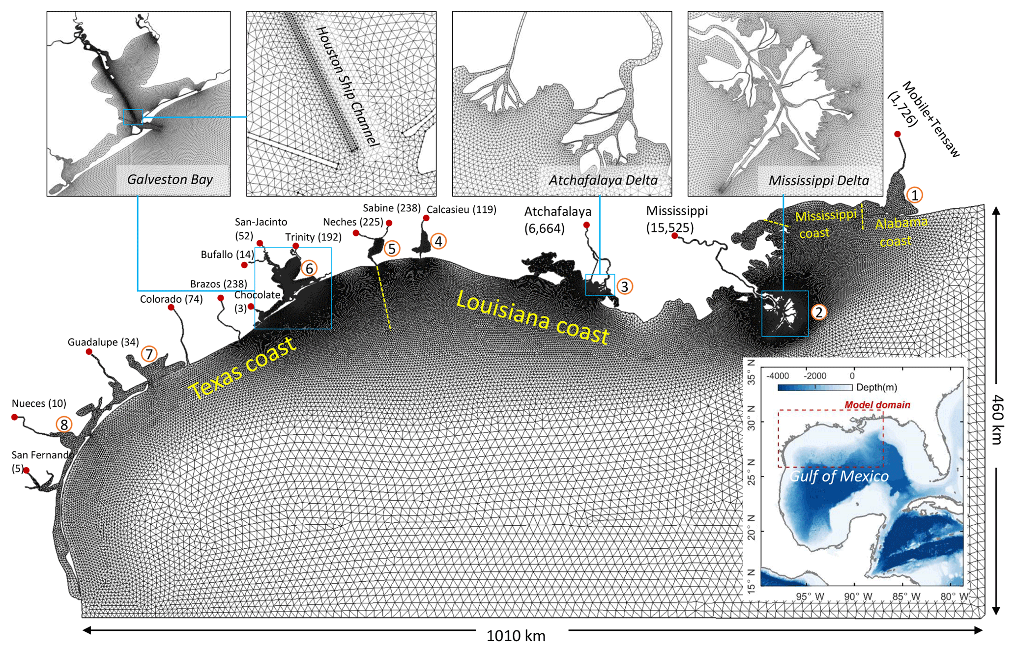
Figure 1The model domain and the horizontal grid, with the upper panels showing zoomed-in views of selected coastal systems. Locations of major river inputs are indicated with red dots, with the associated mean river discharges (m³ s⁻¹) shown in parentheses. Major estuarine bay systems in the model domain include Mobile Bay (1), Mississippi River (2), Atchafalaya River (3), Calcasieu Lake (4), Sabine Lake (5), Galveston Bay (6), Matagorda Bay (7), and Corpus Christi Bay (8).

2.2 Model domain and grid system

The model domain covers the Texas, Louisiana, Mississippi, and Alabama coasts, including the shelf as well as major estuaries (e.g., Mobile Bay, Mississippi River, Atchafalaya River, Sabine Lake, Galveston Bay, Matagorda Bay, and Corpus Christi Bay) (Fig. 1). The domain also includes part of the deep ocean to set the open boundary far away from the shelf to avoid imposing boundary conditions at topographically complex locations. The horizontal grid contains 142 972 surface elements (triangular and quadrangular), with the resolution ranging from 10 km in the open ocean to 2.5 km on average on the shelf (shallower than 200 m) to 40 m at the Houston Ship Channel, a narrow but deep channel along the longitudinal axis of Galveston Bay. The fine grid for the ship channel is carefully aligned with the channel orientation in order to accurately simulate the salt intrusion process (Ye et al., 2018). Vertically, a hybrid s–z grid is used, with 10 sigma layers for depths less than 20 m and another 30 z layers for depths from 20 to 4000 m (20, 25, 30, 35, 40, 50, 60, 70, 80, 90, 100, 125, 150, 200, 250, 300, 350, 400, 500, 600, 700, 800, 900, 1000, 1250, 1500, 2000, 2500, 3000, 4000 m); shaved cells are automatically added near the bottom in order to faithfully represent the bathymetry and thus the bottom-controlled processes. This hybrid s–z vertical grid enables the model to better capture the stratification in the upper surface layer while keeping the computational cost reasonable for simulations of the deep waters. With a time step of 120 s and the second-order finite-volume implicit total variation diminishing (TVD²) scheme for mass transport, it takes about 24 h for a 1-year simulation with 120 processors (Intel Xeon E5-2640 v4).

The bathymetry used in the model is based on the coastal relief model (3 arcsec resolution; https://www.ngdc.noaa.gov, last access: 7 November 2019). The local bathymetry in Galveston Bay is augmented by 10 m resolution digital elevation model (DEM) bathymetric data to resolve the narrow ship channel (150 m wide, 10–15 m deep) that extends from the bay entrance all the way to the Port of Houston. The bathymetry of the ship channels in other rivers, such as the Mississippi, Atchafalaya, and Sabine, is manually set following National Oceanic and Atmospheric Administration (NOAA) navigational charts. The depth in the model domain ranges from 3400 m in the deep ocean to less than 1 m in Galveston Bay (Fig. 2).

Figure 2Bathymetry in the model domain showing zoomed-in views (b–c) of Galveston Bay and its main entrance. Note the log scale (a) for depth because of a very wide range of depth over the entire model domain. Also shown are the NOAA tidal gauge stations (open green circles), TWDB (Texas Water Development Board) salinity monitoring stations (solid black circles), and TABS (Texas Automated Buoy System) buoy stations (black solid triangles).

2.3 Forcing conditions

The model was validated for the 2-year conditions in 2007–2008 and was forced by the observed river discharge, reanalysis atmospheric forcing, and open boundary conditions from global HYCOM output. Daily freshwater inputs from United States Geological Survey (USGS) gauging stations were specified at 15 river boundaries (Fig. 1). For the Mississippi River, the largest in the study area, river discharge at Baton Rouge, LA (USGS 07374000), was used. For the Atchafalaya River, the second largest, the discharge data at the upper river station (USGS 07381490 at Simmesport, LA) were used, but the data before 2009 at this station are not available. However, we found a significant linear relationship between this station and the one near the river mouth (USGS 07381600 at Morgan City, LA) with a 2 d time lag (r² of 0.92) based on the data from 2009 to 2017. The freshwater discharge estimated at Simmesport using this relationship for 2007–2008 was used to specify the Atchafalaya River freshwater input into the Atchafalaya Bay. For the Trinity River, the major river input for Galveston Bay, river discharge at the lower reach station at Wallisville (USGS 08067252) was used, where the mean river discharge (averaged over April 2014 and April 2018) is about 56 % of that at an upper reach station at Romayor (USGS 08066500). This is because the water from Romayor likely flows into wetlands and water bodies surrounding the main channel of the Trinity River before reaching Wallisville (Lucena and Lee, 2017). The river discharge data before April 2014 at the Wallisville station are not available. Similar to the case for the Atchafalaya River, there is a significant linear relationship between these two stations (r² of 0.89 with a 4 d time lag based on the data from 2014 to 2018). The freshwater discharge for 2007–2008 estimated using this relationship was used to specify the Trinity River freshwater input into Galveston Bay. River flows from other rivers were prescribed using the data at the closest USGS stations. Water temperatures at the river boundaries were also based on the data at these USGS stations.

Reanalyzed 0.25^∘ resolution, 6-hourly atmospheric forcing data, including air temperature, solar radiation, wind, humidity, and pressure at mean sea level, were extracted from the European Centre for Medium-Range Weather Forecasts (ECMWF; https://www.ecmwf.int, last access: 7 November 2019). SCHISM uses the bulk aerodynamic module of Zeng et al. (1998) to estimate heat flux at the air–sea interface. Both harmonic tide and subtidal water level were used to define the ocean boundary condition, with the harmonic tide (M2, S2, K2, N2, O1, Q1, K1, and P1) from the global tidal model FES2014 (Carrere et al., 2015) and the subtidal water level from the low-pass-filtered (cutoff period of 15 d) daily global HYCOM output. The model was relaxed during inflow to the HYCOM output at the ocean boundary in terms of salinity, temperature, and velocity.

2.4 Numerical experiments

To investigate the remote influence of the MAR discharge, we conducted three numerical experiments that use the same model configuration as in the realistic 2007–2008 model run except for freshwater discharge, wind forcing, initial salinity condition, and salinity boundary condition. To isolate the influence of the MAR discharge, we considered freshwater discharges (constant long-term means) only for the Mississippi River, Atchafalaya River, and Galveston Bay, with no discharge from other coastal systems. To examine the effect of seasonal wind, we chose the January 2008 and July 2008 winds as representative of winter and summer winds, respectively. The January wind was dominated by northeast–east wind and expected to induce a stronger downcoast (from Louisiana toward Texas) longshore current compared to the predominantly south wind in July (Fig. S1). The initial salinity condition is set to 36 psu throughout the entire domain and for all vertical layers. Salinity at the ocean boundary is set to 36 psu throughout the simulation period.

Differences among the three experiment settings include the following: (1) experiment Jan-G includes only the river discharges into Galveston Bay (259 m³ s⁻¹) and uses the January 2008 wind; (2) experiment Jan-GAM includes Galveston discharge as well as the MAR discharges (22 189 m³ s⁻¹) and uses the January 2008 wind; and (3) experiment Jul-GAM has the same discharges as Jan-GAM but uses the July 2008 wind. In each simulation, the January or July wind was repeated every month, rather than using monthly mean steady wind, in order to take into account the wind variability, which is known to play an important role in shelf circulation (Ohlmann and Niiler, 2005).

3.1 Water level

Model–observation comparisons were made for water level at stations along the coast and inside Galveston Bay. Manning's friction coefficient, which is converted to the bottom drag coefficient for the 3-D simulation in the model, was used as a calibration parameter. The model results with a spatially uniform Manning's coefficient of 0.016 m^1∕3 s⁻¹ show good agreement with the observational data. Overall, the model reproduces both the tidal and subtidal components of water level at tidal gauge stations along the coast as well as inside Galveston Bay (Fig. 3, Table 1, and Fig. S2). The MAE is in the range of 7–8 and 5–7 cm for the total and subtidal components, respectively. The model skill varies spatially, with relatively low skills (0.88) at Pilot Station and Dauphin Island for the subtidal component and high skills (≥0.94) at the stations on the Texas coast, including Galveston Bay, for both the total and subtidal components. It is interesting to note that the model has also simulated the storm surge well during Hurricane Ike (around day 625), one of the most severe hurricanes to hit the Houston–Galveston area in recent years. When applied to investigate the dramatic estuarine response to Hurricane Harvey (2017) in Galveston Bay, this model successfully reproduced the long-lasting elevated water level inside the bay (Du and Park, 2019a; Du et al., 2019b). Simulation of surface elevation is sensitive to topography, bottom friction, boundary conditions, and atmospheric forcings. Some discrepancies are expected due to the assumption of a spatially uniform Manning's coefficient. Further improvement might be achieved by using spatially varying coefficients, but we did not deem it worth trying, considering the current satisfactory performance of the model. Additional discrepancies may come from the limited spatial and temporal resolution of atmospheric forcings, the accuracy of the bathymetric data, and the reliability of the open boundary conditions from the global HYCOM output.

Figure 3Subtidal surface elevation comparison between the model (red line) and observations (black line) at NOAA tidal gauge stations (see Fig. 2 for their locations).

Download

Table 1Error estimates for model–data comparison for 2007–2008.

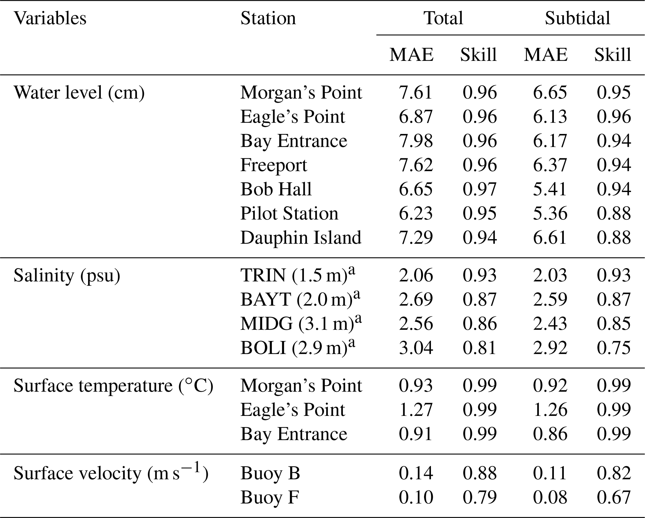
^a The value within parentheses indicates the mean depth of the sensor below the surface.

Download Print Version | Download XLSX

3.2 Salinity

The model reasonably reproduces the observed variation in salinity at stations inside Galveston Bay (Fig. 4 and Table 1). The MAEs are no larger than 3 psu and the model skills range between 0.81–0.93 and 0.75–0.93 for the total and subtidal components, respectively. It is important to note that the salinity at the bay mouth under normal (i.e., non-flooding) conditions is sensitive to the longshore transport of low-salinity water from neighboring estuaries, such as the nearby Sabine–Neches River, Atchafalaya River, and Mississippi River. Successful simulation of salinity at the bay mouth requires an accurate simulation of not only the bay-wide transport, but also the longshore transport. Errors in the modeled salinity at the bay mouth can propagate to the upper bay. For example, salinity during days 60–100 is overestimated at the mouth (station BOLI) and this error propagated into the middle bay station (station MIDG) (Fig. 4). Discrepancies as large as 10 psu are not likely caused by inaccurate discharge from the Trinity River, as this river has a very limited influence on the salinity on the shelf (further discussed in Sect. 4.3). Unfortunately, with no data available for the vertical salinity profile, the model performance for vertical mass transport cannot be evaluated. However, accurate simulation of the observed salinity at the mid-bay station provides alternative evidence supporting the model's validity in horizontal mass transport and salt intrusion.

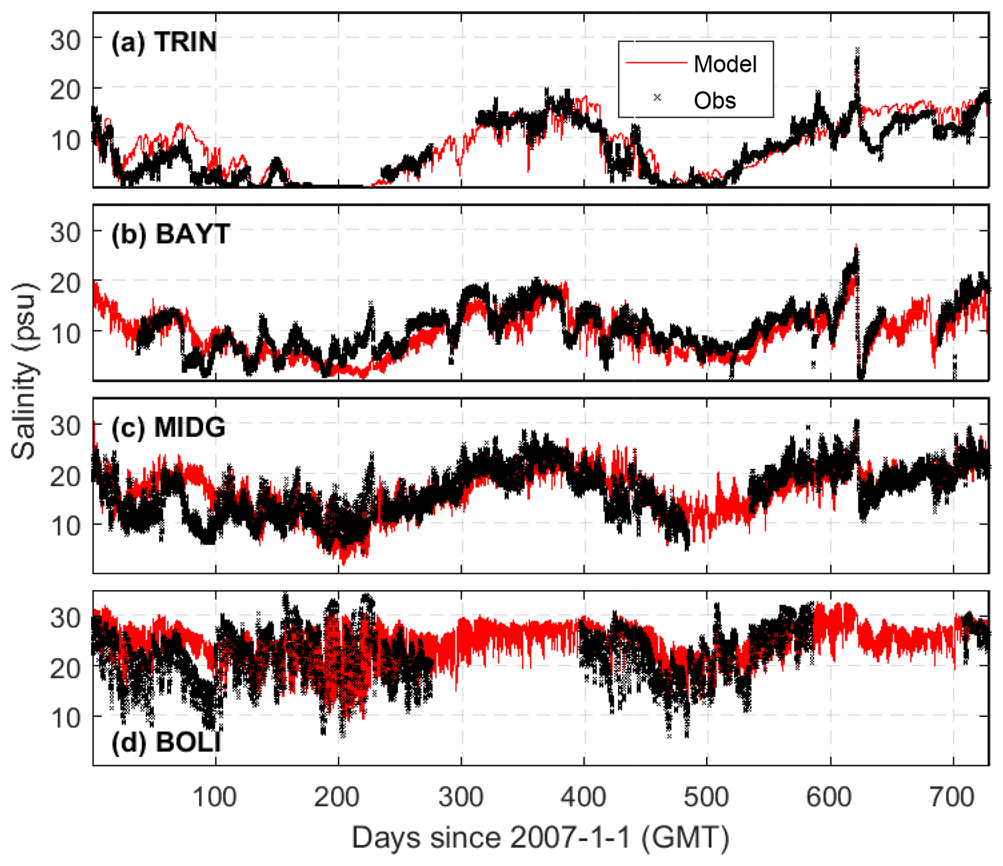
Figure 4Salinity comparison between the model (red line) and observations (black cross) at four TWDB stations (see Fig. 2 for their locations).

Download

The model also captures the sharp change in salinity during Hurricane Ike (around day 620). The salinity at the upper bay (Fig. 4b) decreased from 26 psu to 0 within 2 d, which was caused by a pulse of freshwater discharge from Lake Houston (see reservoir storage at USGS 08072000). In addition, the model reproduces the spatial difference well in the amplitude of the tidal signal in salinity. Salinity in Trinity Bay (Fig. 4a) shows a very weak tidal signal, while salinity at the bay mouth (Fig. 4d) has a much stronger tidal signal. Galveston Bay, in general, has micro-tidal ranges with a mean tidal range of 0.3 m at the mid-bay station (Eagle Point in Fig. 2). The tidal signal, however, becomes stronger at the narrow bay mouth (2.5 km wide), with the tidal current being as strong as 1 m s⁻¹ (see station g06010 at http://pong.tamu.edu/tabswebsite/, last access: 7 November 2019).

The modeled salinity was also compared to the observed salinity structure over the Texas–Louisiana shelf using the data from a shelf-wide summer survey in July 2008 as an example (Fig. 5). Both the horizontal and vertical structures of salinity on the shelf are well reproduced by the model, with an MAE over 65 stations of 1 and 2 psu for the surface and bottom salinity, respectively. Data and the model consistently show a relatively shallow halocline at section A (west of Mississippi Delta) and a deeper halocline at section F (off Atchafalaya Bay). The upper layer off Atchafalaya Bay was nearly well mixed, which is also reproduced by the model, although the model somewhat underestimates the bottom salinity at section F. In addition, the model also shows that there was little tidal variability of the vertical salinity profile on the shelf (e.g., stations F4 and A7 in Fig. 5), which can be attributed to the small tidal range in the northern GoM.

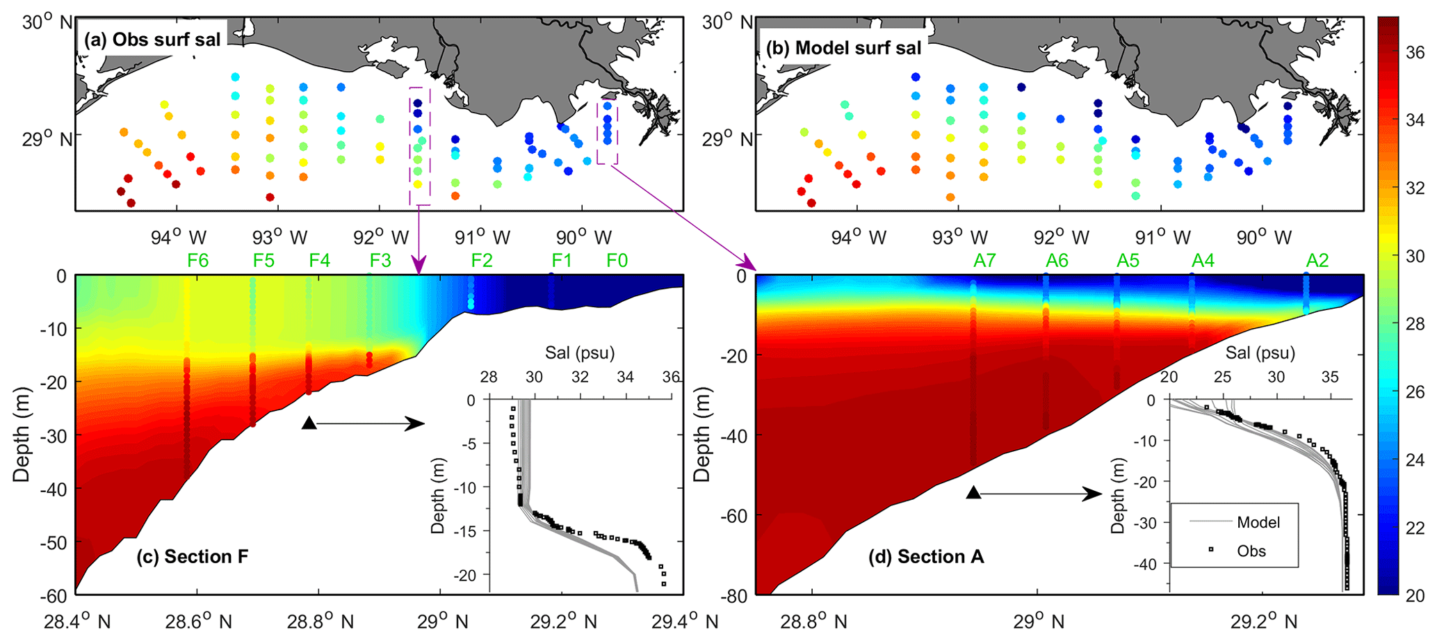
Figure 5Salinity distribution at the Texas–Louisiana shelf from the shelf-wide survey on 22–27 July 2018: comparison of (a) observed and (b) modeled surface salinity and of the vertical profiles at two cross-shelf sections, (c) F and (d) A. In (c) and (d), the colored dots indicate observed salinity, while the filled colors indicate modeled salinity, and the insets compare the vertical profiles of salinity at the selected stations of F4 and A7, respectively. The grey lines in the insets show the 12 modeled profiles over 1 d (observation time ±0.5 d).

3.3 Temperature

The model reproduces the observed temperatures well at three NOAA stations located from the Galveston Bay mouth to the upper bay (Fig. 6). Both the seasonal and diurnal cycles are well captured, with MAEs of about 1 ^∘C and model skills of 0.99. Even within a relatively small region inside Galveston Bay, temperature can vary significantly. During days 300–350, for example, large fluctuations in temperature occurred at the mid-bay station (Fig. 6b), while the fluctuations were smaller at the bay entrance (Fig. 6a) and the upper bay (Fig. 6c). These spatiotemporal variations are reproduced well by the model, demonstrating not only the good performance of the model, but also the reliability of the atmospheric forcing data.

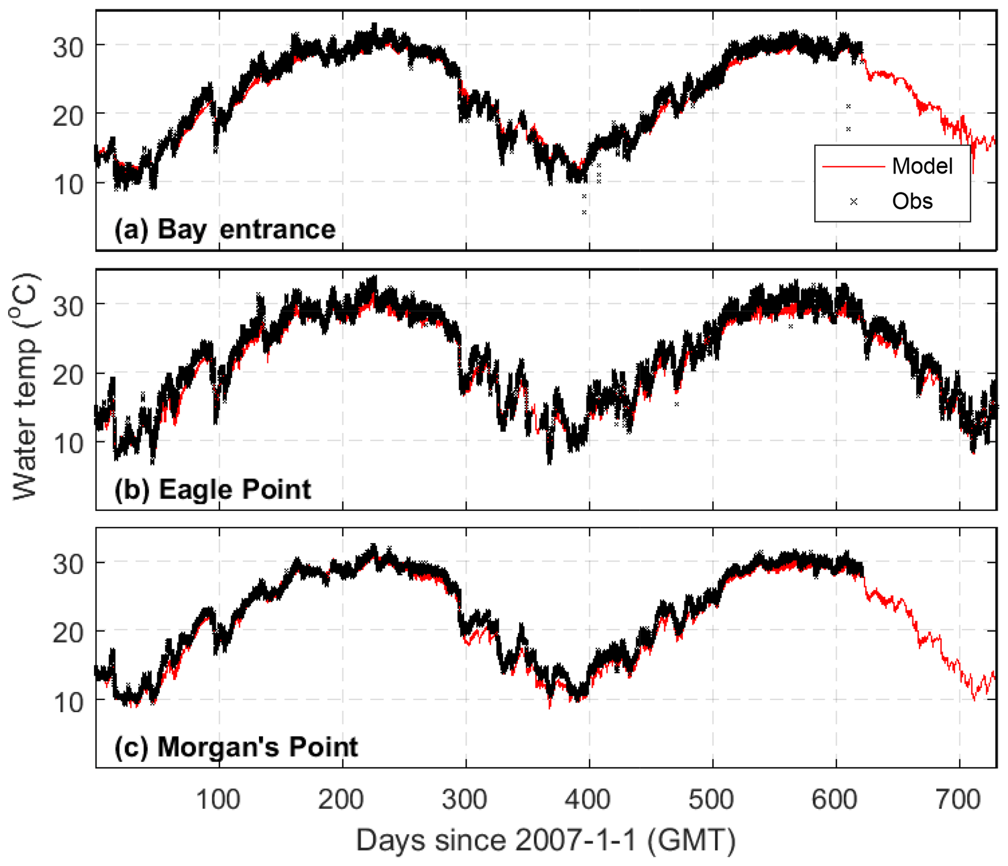
Figure 6Temperature comparison between the model (red line) and observations (black line) at three NOAA stations (see Fig. 2 for their locations).

Download

The model performance in reproducing temperature over the Texas–Louisiana shelf was further examined with satellite data for sea surface temperature (SST). Seasonality of the SST extracted from MODIS over the northern GoM is overall reproduced well (Fig. 7). It is worth noting that the model also reproduces the relatively low temperatures on the southern Texas coast during summer, which is a well-known upwelling zone during the summertime when upcoast (from Texas toward Louisiana) winds drive an offshore surface transport (Zavala-Hidalgo et al., 2003).

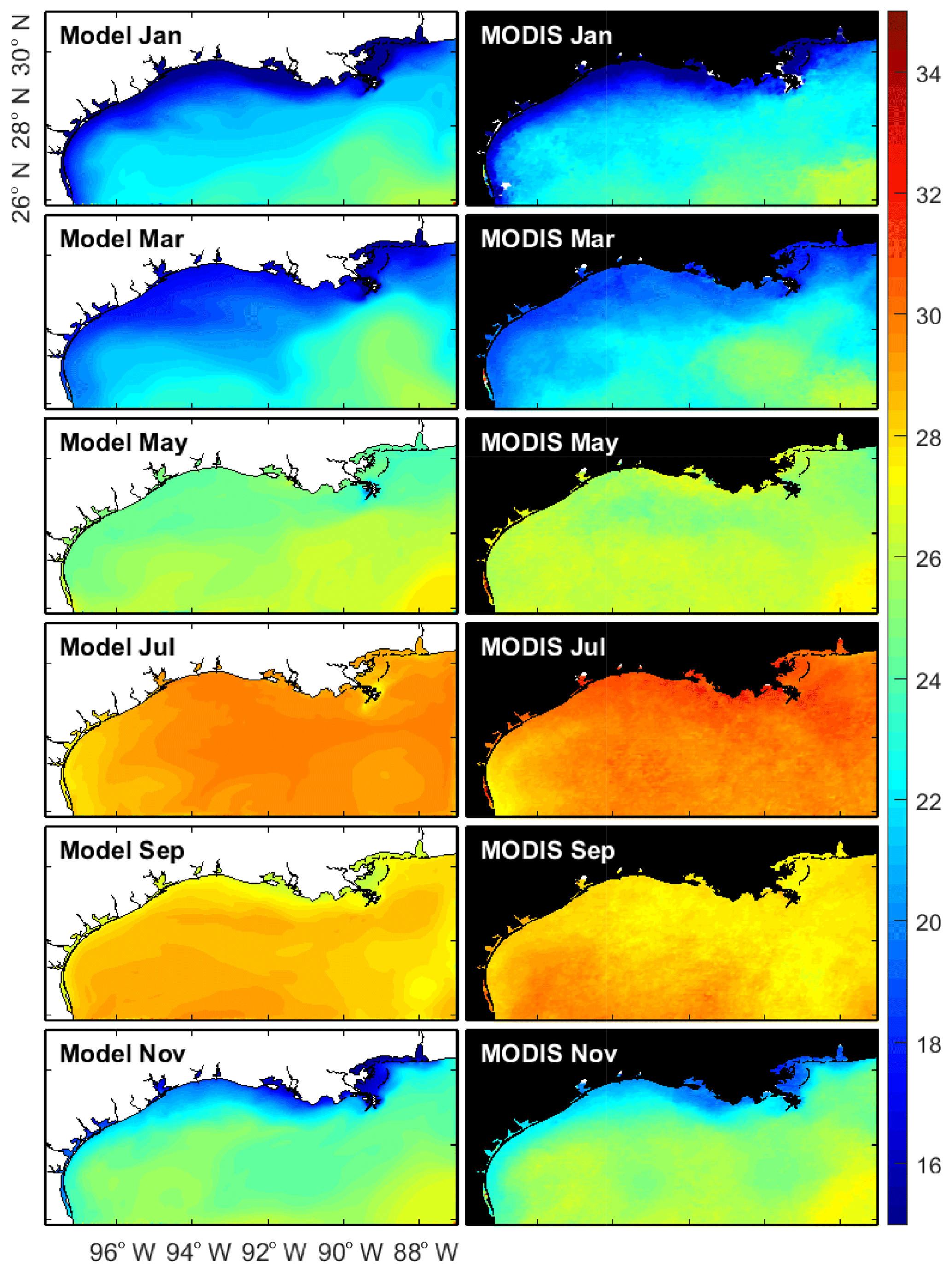
Figure 7Temperature comparison (monthly average) between the model (left panels) and MODIS satellite data (right panels) for selected months in 2008.

3.4 Shelf current

The shelf current plays a key role in transporting low-salinity water originating from MAR, and it can be affected by not only the wind field, but also the mesoscale eddies in the northern GoM. One of the important features of the Texas–Louisiana shelf is the quasi-annual pattern of the shelf current, which is predominantly westward most of the time except during summer (Cochrane and Kelly, 1986; Li et al., 1997; Cho et al., 1998). The prominent downcoast shelf current is driven by along-shelf wind and enhanced by the MAR discharge (Oey, 1995; Li et al., 1997; Nowlin et al., 2005). Under summer wind that usually has an upcoast component, the nearshore current is reversed to the upcoast direction (Li et al., 1997). Such seasonality also occurred during 2007–2008. The model reproduces the observed subtidal component of the surface longshore current at two TABS buoy stations outside Galveston Bay, buoy B (∼20 km offshore) and buoy F (∼80 km offshore) (Fig. 8), with MAEs of 8–14 cm s⁻¹ and model skills of 0.67–0.88 (Table 1).

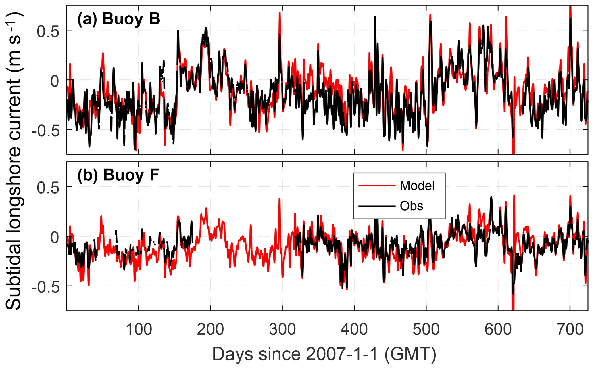
Figure 8Comparison of the subtidal east–west surface shelf current between the model (red line) and observations (black line) at two TABS buoys (see Fig. 2 for their locations).

Download

4.1 Variation in shelf current and salinity

The strength and direction of the shelf current are sensitive to the wind field. Comparison of the model results on day 150 (31 May 2007) and day 160 (10 June 2007) clearly shows the different distribution of lower-salinity water along the coast in response to wind field and the resulting shelf current (Fig. 9). The river discharge differences between these two days are negligible, and thus the differences in lower-salinity water distribution can be mainly attributed to the differences in shelf current. Day 150 was characterized by a significant downcoast shelf current in the inner shelf, with a current speed exceeding 0.5 m s⁻¹, while day 160 was characterized by a rather weak shelf current with a speed of less than 0.1 m s⁻¹. The pattern of the surface residual current is related to the wind field. On day 150, a downcoast component of the wind induced an onshore Ekman transport, which in turn resulted in a downcoast geostrophic flow (Li et al., 1997). This downcoast flow transported low-salinity water from MAR toward Texas while constraining it to a narrow band against the shoreline (Fig. 9e). Under a weak or upcoast shelf current, in contrast, this constraining was weakened, leading to the offshore displacement of low-salinity water (Fig. 9f). As a result, salinity on the Texas inner shelf was higher on day 160 than on day 150.

Regulated by the shelf current, salinity distribution over the shelf exhibits evident seasonality. The model results show that a narrow band of lower-salinity water persisted from Louisiana to the western Texas inner shelf during January–May 2008 (Fig. 10). The salinity at the Galveston Bay mouth decreased by about 10 psu from January to May, which can be attributed to the increasing Mississippi discharge from January to May in 2008 (Mississippi discharge data at https://waterdata.usgs.gov/usa/nwis/uv?site_no=07374000, last access: 7 November 2019). Starting from June 2008, the salinity along the western Texas shelf gradually increased as higher-salinity water from the southwestern boundary moved upcoast. The salinity at the Galveston Bay mouth increased from less than 20 psu in June to >30 psu in August (Fig. 10), about the same magnitude of salinity change from January to May. It suggests that the influence of the seasonally varying shelf circulation on salinity at the Texas coast is comparable to that of the seasonal variation in the MAR discharge.

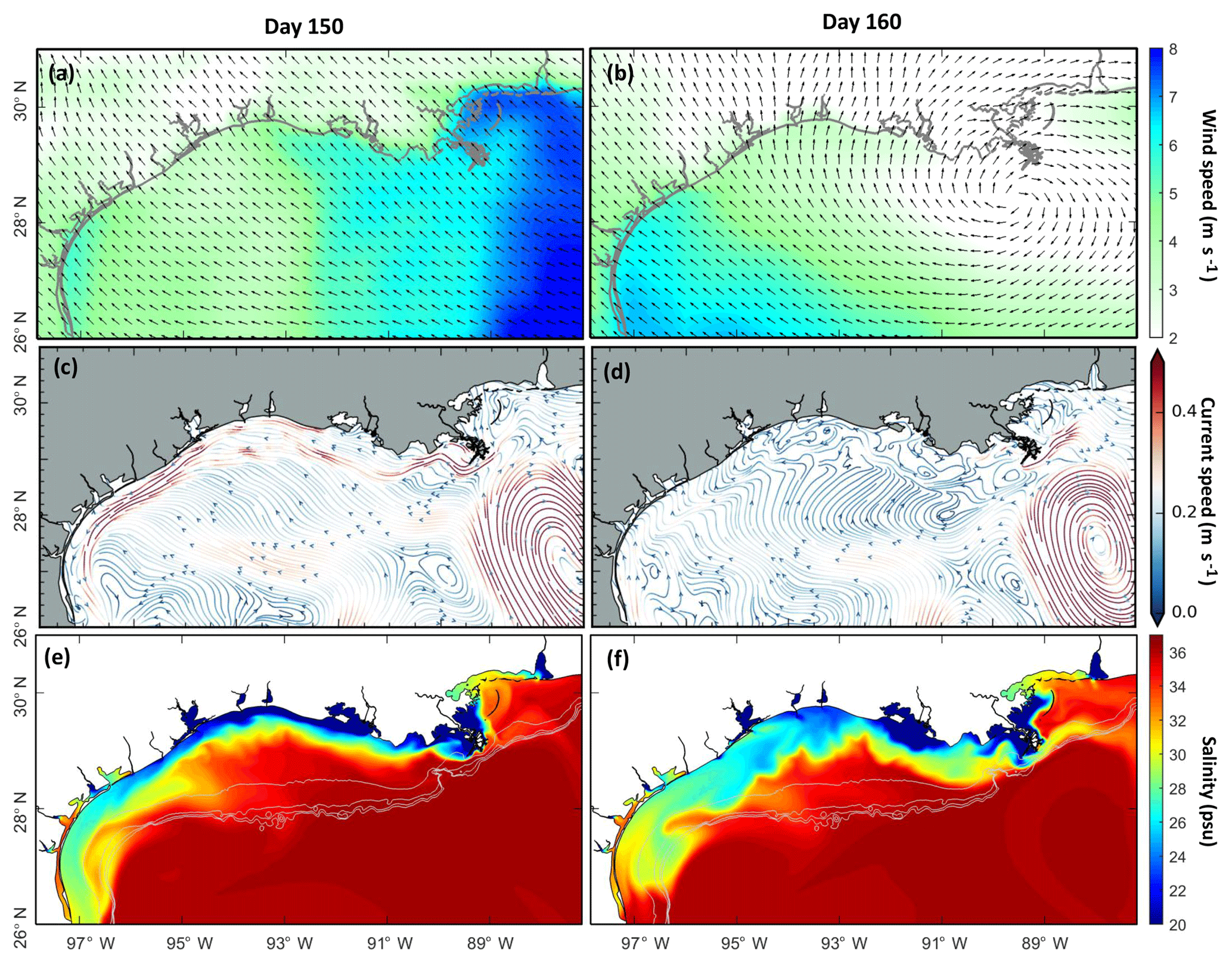
Figure 9Comparison of the observed wind field and the modeled surface residual current and surface salinity on day 150 (31 May 2007) and day 160 (10 June 2017). The filled colors indicate the daily mean wind speed (a, b), the speed of the residual current (c, d), and salinity (e, f).

Figure 10The modeled monthly mean surface salinity in 2008, with the grey contour lines denoting depth contours of 50, 100, 150, and 200 m.

4.2 Influence of the MAR discharge on shelf transport and salinity

Longshore transport plays a key role in redistributing freshwater from the estuarine bays along the shelf. The results from three numerical experiments show that, under the January wind, the downcoast longshore transport among four selected cross-shelf sections varies little. The longshore transport is enhanced by the MAR discharge (long-term mean) by 10 %–14 % (∼80 000 m³ s⁻¹), about 4 times the long-term mean river discharge from MAR (∼22 000 m³ s⁻¹) (Fig. 11). The transport, however, is greatly reduced under the July wind and it decreases downcoast, with the magnitude being 1 order smaller on the Texas shelf compared to that under the January wind. The difference in longshore transport is related to the shelf circulations, which exhibit distinctly different patterns under different wind conditions (Fig. S3). Under the January wind, the surface shelf current flows downcoast, while under the July wind, it is weak and mainly in a direction normal to the coastline, resulting in a much smaller longshore transport.

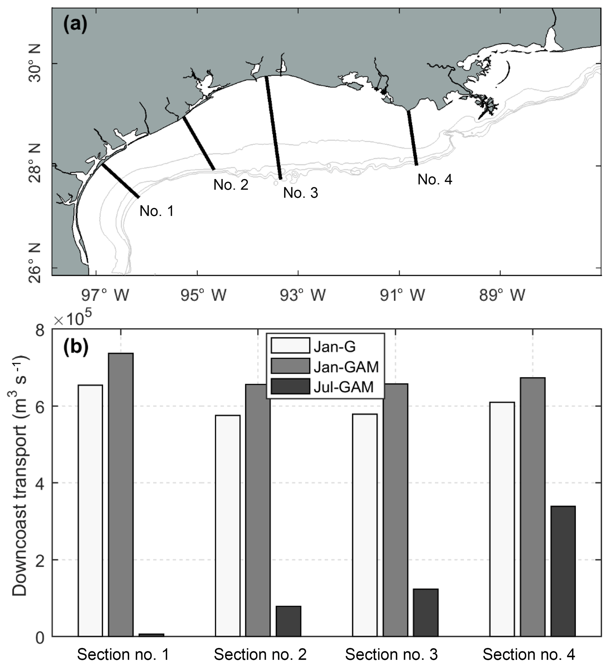
Figure 11Downcoast longshore transport at four selected cross-shelf sections for three numerical experiments with constant long-term mean river discharges: river discharges into Galveston Bay only with January 2018 wind (Jan-G) and the MAR discharge as well as discharges into Galveston Bay with January 2018 wind (Jan-GAM) or July 2018 wind (Jul-GAM).

The influence of the MAR discharge on shelf salinity also depends on the wind condition and the resulting shelf current. Surface salinity maps averaged over days 250–300 show distinctly different spatial patterns of the lower-salinity water under different wind conditions (Fig. 12). The patterns are similar to the results from the 2007–2008 realistic run (Fig. 10). Under the winter wind, lower-salinity water is trapped nearshore by the shelf current, forming a narrow band along the coast. Under the summer wind, on the other hand, water on the Texas shelf is replenished by saltier water originating from the southwest, leading to a tongue-shaped saltier-water intrusion toward the lower-salinity water over the Louisiana shelf. Consequently, salinity is higher on the Texas shelf and lower on the Louisiana shelf when compared to that under the winter wind.

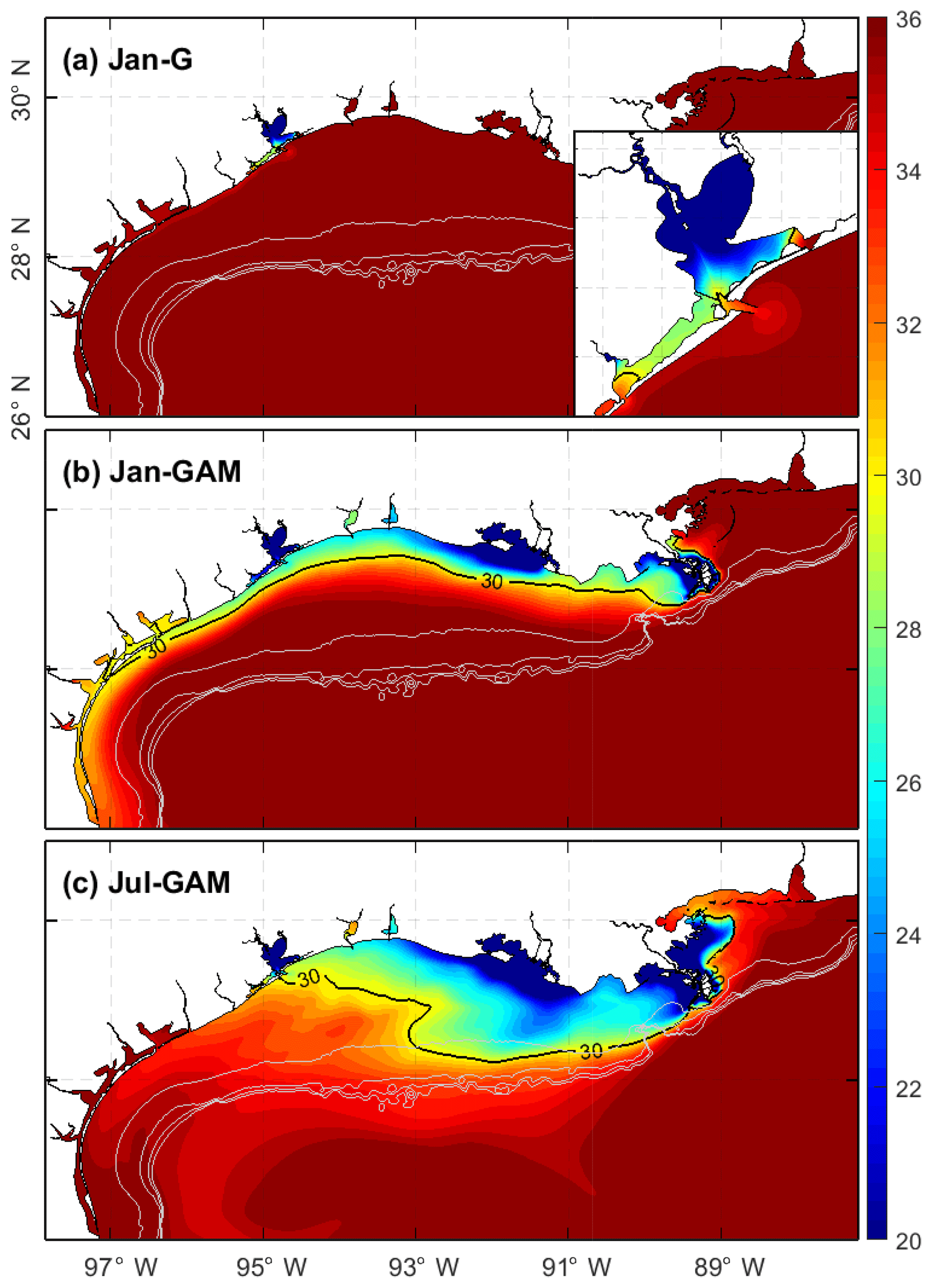
Figure 12Surface salinity distributions averaged over days 250–300 from three numerical experiments. Grey contour lines denote depth contours for 50, 100, 150, and 200 m.

4.3 Influence of the MAR discharge on Texas coast: salinity, stratification, and mixing

Numerical experiments reveal different time and spatial scales with which the surface salinity in Texas coastal water responds to the MAR discharge (Fig. 13). At the Galveston Bay mouth, the salinity begins to decrease from about day 25 in response to the MAR discharge and continues to decrease until around day 100 when it reaches a quasi-steady state. The MAR discharge (long-term mean) reduces the salinity by about 10 psu under the January wind but only by 5–6 psu under the July wind. Further south at the Port Aransas mouth, the response time doubles to about 50 d, with the MAR discharge reducing the salinity by about 6 psu under the January wind. Salinity changes little in response to discharges from Galveston Bay and the MAR discharge under the July wind. As the influence from Galveston Bay is very limited at the Aransas Bay mouth even under a downcoast wind, it is reasonable to assume the influence will be even smaller under an upcoast wind.

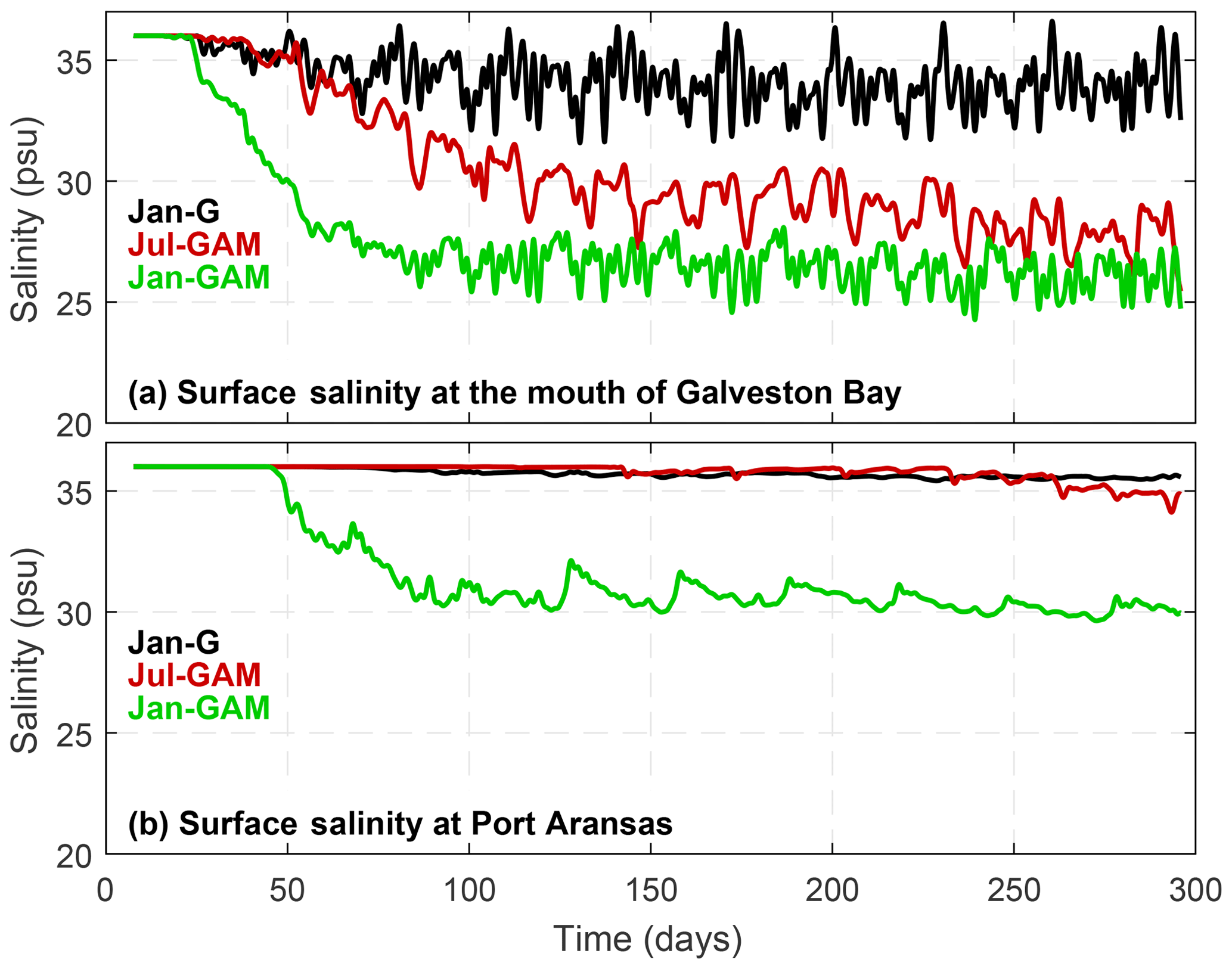
Figure 13Subtidal surface salinity at the mouth of (a) Galveston Bay and (b) Aransas Bay for three numerical experiments.

Download

Vertical profiles of salinity along a section from the Trinity Bay, along the Houston Ship Channel and the adjoining shelf, show that the MAR discharge increases salinity stratification on the shelf (Fig. 14). The lower-salinity water along the coastline increases the cross-shelf baroclinic pressure gradient, leading to a stronger stratification. There is a distinctive difference between Jan-GAM and Jul-GAM. A stronger stratification on the inner shelf appears under the July wind, with the bottom-surface salinity difference as large as 4 psu. Vertical mixing on the inner Texas shelf is weakened due to the MAR discharge, particularly under the July wind. The vertical diffusivities are 1 or 2 orders of magnitude smaller than those under the January wind. Under the July wind, the stratification along the ship channel becomes stronger, probably because of higher salinity near the bay mouth and/or a weaker wind in July with a mean speed of 4.79 m s⁻¹ relative to a mean speed of 6.88 m s⁻¹ in January (Fig. S1). Higher salinity near the mouth induces a stronger horizontal salinity gradient, leading to stronger circulation and stratification.

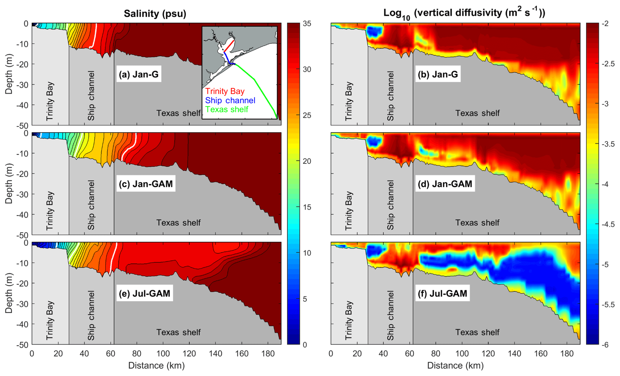
Figure 14Salinity (a, c, e) and vertical diffusivity (b, d, f) averaged over days 250–300 from three numerical experiments for the section through Trinity Bay, the Galveston Bay ship channel, and the Texas shelf: see the inset in (a) for the section location. In (a), the bold white lines denote salinity contours of 10, 20, and 30 psu.

4.4 Influence of the MAR discharge on estuarine–coastal exchange

Salinity change due to remote river input and a shift in the wind field affects the estuarine dynamics, such as estuarine circulation, salt flux, and estuarine–coastal exchange. We examined the change in exchange flow and salinity at the Galveston Bay mouth due to remote river influence and a different shelf current. Following Lerzak et al. (2006), we calculated the tidally averaged and cross-sectionally varying components (u_e and S_e) from the along-channel velocity u and salinity S. From the vertical profiles of u_e and S_e at the deepest part between the two jetties at the bay mouth, it is evident that in the lower layer u_e is strongest (maximum of 6 cm s⁻¹) and S_e is largest (maximum of 0.95 psu) for the case Jan-G, indicating the strongest exchange flow (i.e., estuarine circulation) compared to the other two cases with the MAR discharge (Fig. 15). In contrast, the case Jan-GAM shows the weakest bottom u_e (maximum of 4 cm s⁻¹) and the smallest bottom S_e (maximum of 0.60 psu). The MAR discharge under the January wind condition decreases the salinity at the bay mouth the most and results in the weakest horizontal salinity gradient and exchange flow.

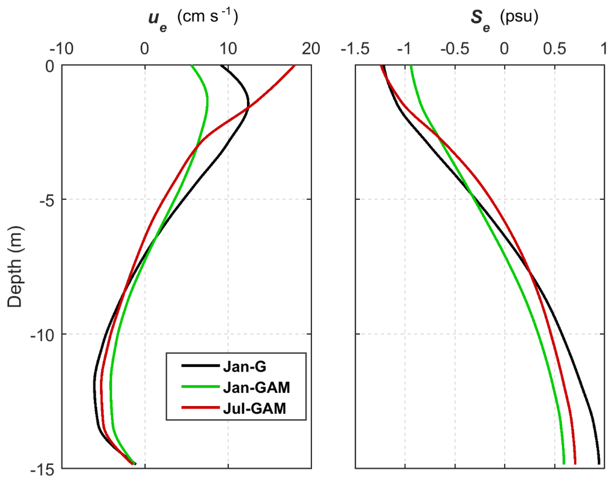
Figure 15Vertical profiles of exchange flow (u_e) and salinity (S_e) at the deepest part of the Galveston Bay mouth averaged over days 250–300 for three numerical experiments.

Download

The influence of the MAR discharge on the dynamics of Galveston Bay was further examined with total exchange flow (TEF) using the isohaline framework method proposed by MacCready (2011), which was found to be a precise way to quantify landward salt transport (Chen et al., 2012). In this method, the tidally averaged volume flux of water with salinity greater than s is defined as

where A_s is the tidally varying portion of the cross section with salinity greater than s. In our case, we calculated Q(s) for the salinity bins from 0 to 35 psu with an interval of 0.5 psu. The volume flux in a specific salinity class is defined as

where the minus sign indicates that a positive value of $-\partial Q$/∂s corresponds to inflow for a given salinity class. The total exchange flow (Q_in), the flux of water into the estuary due to all tidal and subtidal processes, is then calculated as

The resulting salt flux into the estuary (F_in) is given by

and the ratio of salt mass inside the estuary to the salt influx gives the mean residence time (T_res):

where V is the estuarine volume.

Table 2 lists the values of Q_in, F_in, and T_res for three numerical experiments. For the exchange flow, Q_in is largest for the case Jan-G and smallest for the case Jan-GAM. The MAR discharge under the January wind condition causes the largest decrease in salinity at the Galveston Bay mouth (Fig. 13a), effectively slowing down the water exchange between the bay and coastal ocean. The reduction in Q_in caused by the remote discharge (470 m³ s${}^{-\mathrm{1}}=\mathrm{24}$ % reduction) is 1.8 times the long-term mean river input into Galveston Bay (259 m³ s⁻¹). Moreover, F_in for the case Jan-GAM is about half of that in the case Jan-G. As a result, T_res of the bay is largest in the case Jan-GAM, although the difference in T_res is not as large as that in F_in because the bay has the smallest salt mass in the case Jan-GAM (Table 2). This analysis also suggests that the exchange between the bay and coastal ocean is likely stronger during summer than during winter under the same river discharge condition.

Table 2Total exchange flow (Q_in) and the resulting salt flux (F_in) at the Galveston Bay mouth, as well as the mean residence time of the bay (T_res) based on the isohaline method in MacCready (2011).

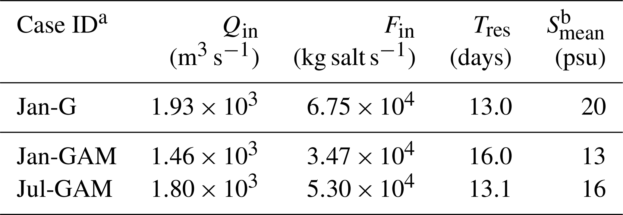
^a See Fig. 11 for an explanation of idealized runs. ^b Mean salinity (volume-weighted average over days 250–300) inside the bay.

Download Print Version | Download XLSX