In February 2009, 76 kg of the inert tracer trifluoromethyl sulfur pentafluoride (CF₃SF₅) was released at the potential density (referenced to 1000 m) of 32.325 kg m⁻³ (neutral density ≈27.9 kg m⁻³; depth ≈1500 m) near 58^∘ S, 253^∘ E. The tracer was chosen as it has a very low background atmospheric concentration and nearly negligible interior ocean concentration, is non-toxic and is chemically inert in the environment, and is detectable at extreme dilution (Ho et al., 2008). The tracer was released in a cross pattern approximately 20 km wide, between the Subantarctic and Polar fronts and at the density of Upper Circumpolar Deep Water. The initial tracer distribution, determined by sampling within 2 weeks of the release, was found to be centred about 4 m below the target density surface. The rms spread of the tracer in density was documented as approximately 0.0015 kg m⁻³, corresponding to a vertical rms spread of 5.5 m. For details of the release method and measurement technique, see Ledwell et al. (2011).

Several subsequent surveys were undertaken: in February 2010 in the region 57 to 62^∘ S and 255 to 275^∘ E (Fig. 1a); in December 2010 (Fig. 1b), April 2011 (Fig. 1c) and August 2011 (Fig. 1d) in the regions west of and at Drake Passage; and along the western and northern margins of the Scotia Sea in 2012 (February–March, Fig. 1e) and 2013 (March–April, Fig. 1f) to measure the change in distribution of the tracer with time. Tracer sampling and shipboard chemical analysis are described in Ledwell et al. (2011) and in Watson et al. (2013).

We have analysed 11 sections taken at 5 locations, here named as follows: South Pacific (actually a regional survey), south-east Pacific (along 282^∘ E), Drake Entry (near 293^∘ E), Drake exit (along the section commonly termed SR1b near 303^∘ E), and North Scotia (along the North Scotia Ridge). These locations are indicated in Fig. 1.

Figure 1(a–f) Cast locations for each summer voyage in which tracer measurements were taken. The size of each marker corresponds to the peak tracer concentration for that cast. Marker sizes are scaled relative to the largest measured tracer concentration for that time period (i.e. markers corresponding to the cast where the largest concentration was measured have the same size between all six figures; see Fig. 2 for maximum concentrations for each section). The star indicates the release location, upward triangles the South Pacific region (US Voyage 2), diamonds the south-east Pacific section (along 282^∘ E), circles the Drake Entry section (along Phoenix Ridge), downward triangles the Drake exit section (otherwise known as SR1b) and right triangles the North Scotia section. (g) Salinity observations interpolated onto the release isopycnal surface (circles). A spline fit of the mean latitude of salinities between 34.645 and 34.65 g kg⁻¹ is shown with a black line.

Figure 2(a) The peak concentration measured (log₁₀ mol L⁻¹) at each section as a function of time since release (months). (b) Peak depth-integrated concentration (log₁₀ mol m L⁻¹). Although higher concentrations could be inhomogeneously distributed either side of the sections at a given time, the time series suggests that the concentration peak is closer to the eastern South Pacific before 30 months and closer to or beyond the North Scotia Ridge by the last transect near 50 months.

Download

Year on year, the tracer was found increasingly toward the east and in lower concentrations (Fig. 2; Watson et al., 2013). The tracer closely followed the release isopycnal surface, spreading slowly across isopycnal surfaces (i.e. across vertically stacked density layers). Tracer profiles averaged over sections as a function of density and then transformed into depth coordinates through a reference density–depth profile were approximately Gaussian. The spread of these Gaussian profiles with time and/or with distance to the east yielded diapycnal diffusivities of O($\mathrm{2}\times {\mathrm{10}}^{-\mathrm{5}}$) m² s⁻¹ in the South Pacific (Ledwell et al., 2011; Watson et al., 2013) and O($\mathrm{3}\times {\mathrm{10}}^{-\mathrm{4}}$) m² s⁻¹ in the Scotia Sea, where the ACC flows over comparatively shallow and complex topography (Watson et al., 2013).

The tracer was not always delimited at the northern and southern ends of the transects or surveys due to compromises dictated by ship time limitations. Sampling was planned with information on the locations of the Polar Front to the south and the Subantarctic Front (west of Drake Passage) or of the continental slope (east of Drake Passage) to the north. The tracer had been released midway between the two fronts, and so when compromises in sampling were needed, sampling was curtailed beyond the fronts, especially north of the Subantarctic Front in the Pacific, guided by the notion that the fronts are barriers to cross-ACC transport (e.g. Naveira Garabato et al., 2016) and also by an altimetry-based prediction of tracer patch spreading. It turned out that little tracer was detected south of the Polar Front when time allowed for sampling there. However, sections in the Pacific often found high concentrations in the northernmost (although still south of the Subantarctic Front) stations, suggesting that there was tracer to the north of the sampled area. In fact, the evidence is that not very much of the tracer spread to the north of the Subantarctic Front. The DIMES float trajectories, shown in Fig. 3 of LaCasce et al. (2014), illustrate that virtually none of the floats went far enough north to avoid transiting through Drake Passage. The ensemble of numerical simulations for realistic conditions, calibrated with the available tracer observations, shown in Fig. 1 of Tulloch et al. (2014) also suggests that relatively little tracer was missed to the north or south of the sampled regions. Hence, we argue that tracer sampling was sufficiently representative to support our main conclusions, although the shortfall of sampling adds to the uncertainty of our quantitative analysis.

The tracer was apparently distributed over a smaller meridional range at the Drake Passage exit section than in the south-east Pacific. This could be due to a decrease in meridional spread as the tracer moves downstream associated with the contraction of the ACC as it flows through Drake Passage or due to sampling issues. In either case it poses a problem to conventional analysis of cross-ACC dispersion in terms of a Fickian eddy diffusivity since the second moment in geographical space decreases with time. We shall see shortly that analysis of the along-isopycnal spreading of the tracer into waters with different salinities helps to circumvent this problem.

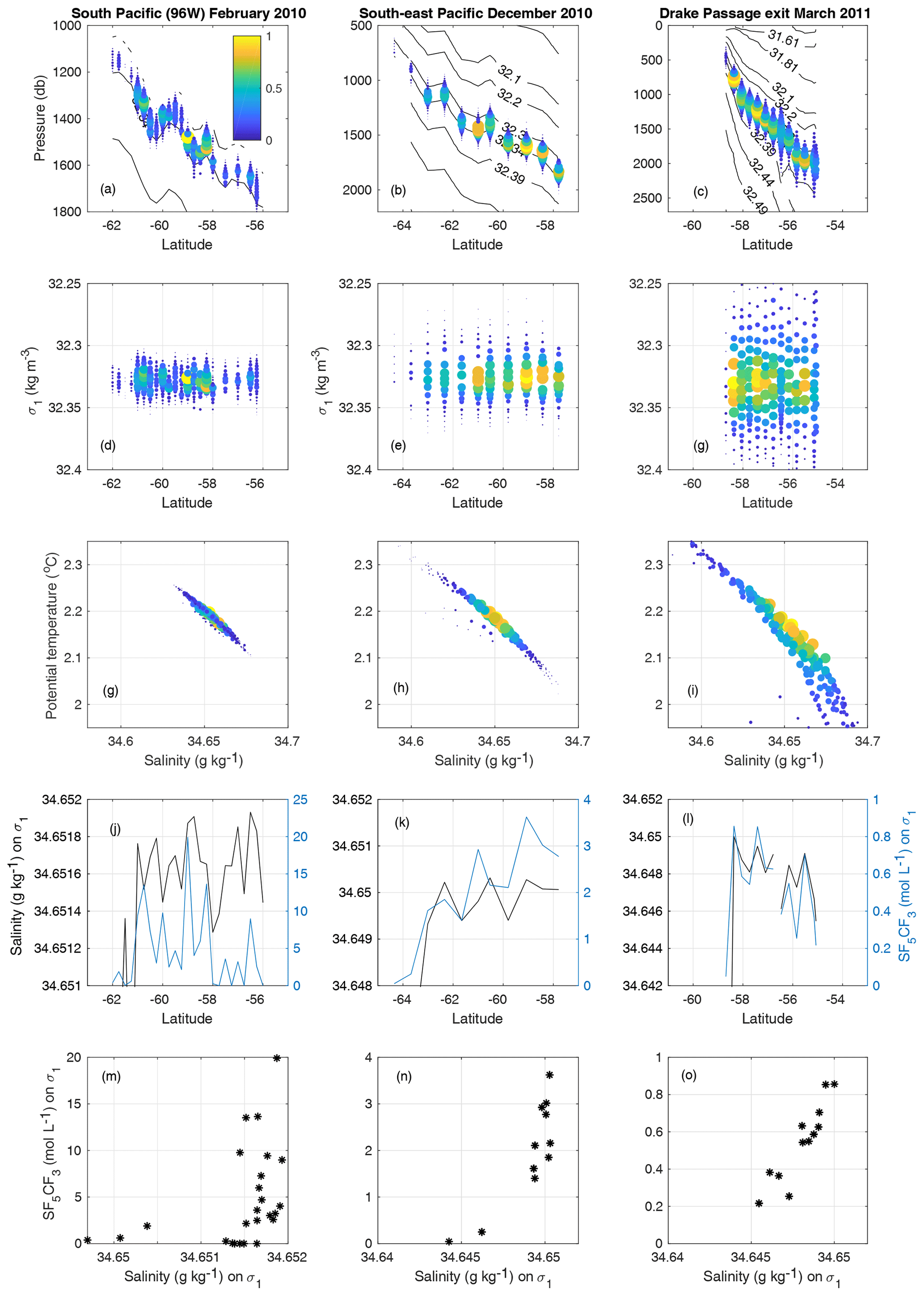
Figure 3(a–c) Depth and latitude of tracer measurements, with contours of potential density referenced to 1000 m (σ₀; not evenly spaced). The Polar Front and the Subantarctic Front are where the slope of the density surfaces is large, near the southern and northern ends of these sections. (d–f) Potential density and latitude of tracer measurements. (g–i) Potential temperature and salinity. (j–l) Salinity and tracer on the σ₁=32.325 kg m⁻³ surface. (m–o) Scatter plot of salinity and tracer concentration on the σ₁=32.325 kg m⁻³ surface (note the changing y axis range). For panels (a)–(i), colour represents tracer concentration relative to the peak measured for that section. Panels (a), (d) and (g) are from the South Pacific cruise of February 2010; (b), (e) and (h) the south-east Pacific section of December 2010; (c), (f) and (i) the Drake exit section of March 2011.

Download

Figure 4Data from all 11 sections from the five DIMES cruises discussed are shown in potential density-versus-isopycnal-salinity-anomaly coordinates. Each point is coloured by the tracer concentration relative to the maximum of that section (see Fig. 2 for these values). Grey contours show the σ∕2, σ and 3σ∕2 contours of a fit of a 2D Gaussian curve to these data.

Download

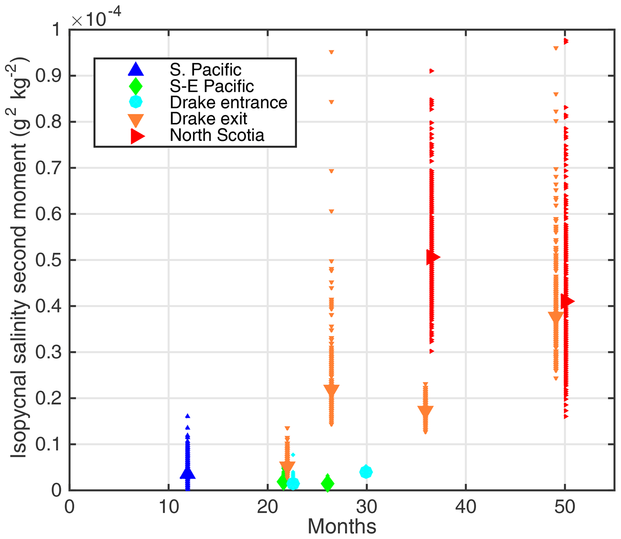
Figure 5Isopycnal second moment of the tracer in salinity coordinates derived from the Gaussian fits in Fig. 3 versus time since release. Each small marker (making up the error bars) represents a single member of the bootstrap ensemble, and the larger marker the result of using all the data.

Download

The tracer was found to spread inhomogeneously in the horizontal. Figure 3 shows the distribution of the tracer as a function of latitude and depth (panels a–c) and latitude and density (d–f) and in temperature and salinity coordinates (g–i) for the South Pacific section in February 2010 (a, d and g), the south-east Pacific section in December 2010 (b, e and h) and the Drake exit section in March 2011 (c, f and i).

The tracer spread isopycnally and formed multiple peaks in concentration, suggesting that the patch had been teased into filaments. When the tracer distribution is projected onto temperature-versus-salinity coordinates, these individual maxima are not seen, suggesting that filaments largely preserve their temperature and salinity values. To investigate this effect further, we show both the salinity and tracer concentration on the release isopycnal (Fig. 3j–l). These two variables are also plotted against one another as a scatter plot (Fig. 3m–o). Two to three years into the experiment (i.e. during the late 2010 and 2011 voyages), higher tracer concentrations are found where the highest salinities are measured on the isopycnal. The core of the tracer is apparently moving with or close to the salinity maximum on the isopycnal.

On an isopycnal surface, the isopycnal salinity anomaly (S^′) is defined as the local salinity minus some reference salinity (S₀). We define S₀ on each density layer to be the salinity at the cast where the largest tracer concentration is measured. In order for the tracer to disperse in this coordinate, it must either cross isohalines at constant density (i.e. changing salinity with a compensating change in temperature) or cross isopycnal surfaces. Our focus here is on dispersion in the isopycnal direction.

We define S₀ separately for each section, rather than as the salinity value on which the tracer was injected. This is in part because as denser and lighter isopycnals are reached by the tracer, their reference salinity may change, and in part to account for migration of the peak due to gradual along-isopycnal transport. On the release isopycnal S₀ remains close to 34.65 g kg⁻¹ throughout our study domain. S₀ appears to decrease slightly toward the east, but the trend is not robust and S₀ is always larger than 34.645 g kg⁻¹.

In Fig. 4, the tracer distributions for each section are mapped onto density-versus-salinity-anomaly coordinates. While in geographical coordinates the dispersion of the tracer has multiple maxima and minima and appears to contract meridionally with time, in density-versus-salinity-anomaly coordinates the tracer spreads out more monotonically.

In order to quantify the spreading of the tracer in isopycnal salinity anomaly coordinates, we apply a non-linear least-squares fit (using Matlab's fminsearch algorithm) of a two-dimensional Gaussian distribution in that reference frame. This is done at each section to yield the standard deviation of salinity in the along-isopycnal direction. As mentioned above, growth of the tracer patch in the diapycnal direction during the initial 2 years of the experiment was analysed by Ledwell et al. (2011) and by Watson et al. (2013) and further discussion of diapycnal mixing is left to future work.

The evolution of the second moment of the tracer in isopycnal salinity anomaly coordinates (the square of the standard deviation) is shown in Fig. 5. There is an apparent weak spreading of the tracer in the first 24 months, with the tracer patch growing to second-moment values generally less than $\mathrm{5}\times {\mathrm{10}}^{-\mathrm{6}}$ (g kg⁻¹)²; then, over the subsequent 24 months, more rapid spreading of the tracer occurs, reaching second-moment values of the order of $\mathrm{5}\times {\mathrm{10}}^{-\mathrm{5}}$ (g kg⁻¹)².

To account for the various sources of sampling error, we estimate uncertainty using the following bootstrapping method. For each section, the tracer observations are randomly subsampled allowing for repeated sampling of the same data. For a section with N samples, N observations are chosen at random (with repetition), and the second moment is determined . This is then repeated N times. Each estimate is shown in Fig. 5.

The uncertainty analysis reveals a larger range of second-moment estimates for the initial South Pacific survey after 12 months than in surveys conducted after 20–30 months in the same region, potentially indicating an initial lack of correspondence between salinity and tracer filaments (Fig. 5). Uncertainties then increase for the later period and in the Scotia Sea, likely due to reduced tracer concentrations, poor coverage of the Gaussian distribution and a lack of consistency of the Gaussian model due to anisotropic variations in mixing and a changing background salinity and density field.

Nonetheless, there is a notable increase in the rate at which the tracer spreads in isopycnal salinity anomaly coordinates between the initial 2 years and the subsequent years of the experiment. This could be explained by the natural phases of evolution of the tracer patch, a change in the rate at which the tracer is mixed or by a change in background salinity gradient. In the next section, we investigate these explanations.

In order to interpret our analysis in terms of geographical dispersion, we next relate the isopycnal salinity anomaly coordinate to an equivalent cross-stream distance. We use the climatological mean distance between isohalines along the ACC to effect this transformation. Although such a transformation results in information loss relating to the moving salinity coordinate, it is instructive in linking dispersion to an apparent mixing coefficient for comparison with other work.

Distances between isohalines are determined using the entirety of available hydrographic data for the region. The hydrographic compilation used in this study includes ship-based observations from the World Ocean Database (http://www.nodc.noaa.gov/OC5/SELECT/dbsearch/dbsearch.html, last access: 9 March 2020) and from the Argo programme (http://www.argo.ucsd.edu, http://argo.jcommops.org, last access: 9 March 2020), as well as from ship-based observations directly obtained from individual principal investigators (PIs) (see Sallée et al., 2010). Ideally, distances between isohalines would be determined for the precise period of the DIMES experiment, but due to data sparsity we have used the entire database.

For each vertical cast, potential density and salinity are determined. Salinity is then linearly interpolated onto the σ₁=32.325 kg m⁻³ isopycnal surface (Fig. 1f). Maps of these raw salinity values show a clear ridge of high salinity running along the ACC on this isopycnal. Higher salinity gradients are apparent further to the east as the ACC contracts. It is along this ridge that the tracer is released.

If fine-resolution (e.g. eddy-resolving), real-time and realistic salinity data were available on the isopycnal surface, we would form a time-varying salinity coordinate by calculating the area contained between salinity ranges and remap this onto a quasi-meridional distance (e.g. following Marshall et al., 2006). However, such a density of data is not available from an observational product. Instead, we estimate the distance coordinate directly from the in situ data. We do this by, first, estimating the mean location of the salinity contour along which the tracer is centred and, second, calculating the average distance from that contour to other salinity measurement sites.

The western South Pacific and South Atlantic are partitioned into seven bands between longitudes 250, 260, 270, 280, 290, 300, 310 and 320^∘ E. Within each band, we determine the average latitude of salinity observations that fall between 34.645 and 34.65 g kg⁻¹ (using a simple arithmetic mean). This defines a latitude (y₀(x)) for each of the seven bands and effectively determines the approximate path the tracer would follow if it did not mix irreversibly. We use 10^∘ and not narrower bands to avoid noise arising from a minimal number of salinity observations being made on the isopycnal. A smooth set of points every 0.5^∘ of longitude are then used to define the curve for y₀(x), using a one-dimensional cubic spline interpolation.

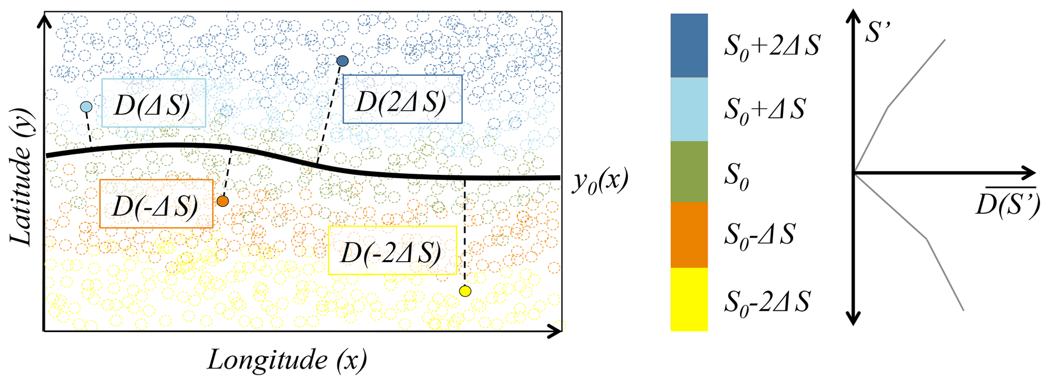
Figure 6Schematic describing the method by which the mean distance as a function of salinity anomaly ($\stackrel{\mathrm{‾}}{D\left(S^{\prime }\right)}$) is calculated. Circles represent salinity observations on an isopycnal surface. The latitude of observations close to the target salinity ($S_{\mathrm{0}}\pm \mathrm{\Delta }S/\mathrm{2}$; green) are used to define a locus of latitudes (y₀(x); solid line). The minimum great-circle distance (D) of each observation from y₀(x) is then determined and binned as a function of the salinity anomaly ($S^{\prime }=S-S_{\mathrm{0}}$). Distances are averaged within each bin, giving a relationship between salinity anomaly and distance $\stackrel{\mathrm{‾}}{D\left(S^{\prime }\right)}$.

Download

For each isopycnal salinity anomaly observation (S^′) we determine its distance (D(S^′)) from the curve y₀(x). Distance is defined as the minimum great-circle distance from the observation to a point on the curve y₀(x). The mean distance, $\stackrel{\mathrm{‾}}{D\left(S^{\prime }\right)}$, is then the average of D(S^′) for a given band of longitudes and over a range of salinities close to S^′. $\stackrel{\mathrm{‾}}{D\left(S^{\prime }\right)}$ is used to transform the salinity anomaly coordinate into an equivalent distance coordinate. In regions where y₀(x) follows a line of constant latitude (as is approximately the case in the South Pacific), $\stackrel{\mathrm{‾}}{D\left(S^{\prime }\right)}$ is effectively the average meridional distance of water parcels with salinity S^′, from the line y₀(x). D(S^′) is averaged within each 10^∘ band and within salinity bins of 0.005 g kg⁻¹, as shown in Fig. 7b.

Our distance coordinate is analogous to other pseudo-distances used in diffusivity studies in the Southern Ocean, where quasi-stream-following coordinates are used. For example, Naveira Garabato et al. (2011) use a similar approximate conversion between dynamic height and latitudinal distance when estimating eddy stirring length scales. It should be noted that there is some unavoidable loss of spatial information in the use of water-mass-following coordinates. While the distance coordinate aims to relate changes in salinity at constant density to changes in distance, it is impossible to know the actual path taken by tracers, and so the distance conversion will always be approximate. We discuss the impact of changes in both the distance coordinate with longitude and their impact on apparent diffusivity in the next section.

The distance $\stackrel{\mathrm{‾}}{D\left(S^{\prime }\right)}$ decreases substantially between the South Pacific and the Scotia Sea. At the release site in the South Pacific waters become 0.01 g kg⁻¹ fresher over approximately 700 km, while they change by the same amount over only 300 km in the Scotia Sea.

In order to translate the salinity second moment (Fig. 5) into units of distance squared (as relevant to the estimation of a mixing coefficient), we construct “reference profiles” based on $\stackrel{\mathrm{‾}}{D\left(S^{\prime }\right)}$. The use of a reference profile is routine when converting isopycnally averaged tracer observations into vertical distance for the purpose of inferring a vertical diffusivity (Ledwell et al., 1993). Since there is a substantial change in the salinity gradient between the South Pacific and the Scotia Sea, and there is an apparent change in the rate at which the tracer spreads in salinity after 18–24 months, we have defined three mean profiles for the entire region between 250 and 310^∘ E, a western region between 250 and 290^∘ E, and an eastern region between 280 and 310^∘ E. The choice of longitudes here is arbitrary, and our aim is to merely assess the sensitivity of second moments and diffusivities estimated to a range of possible profiles.

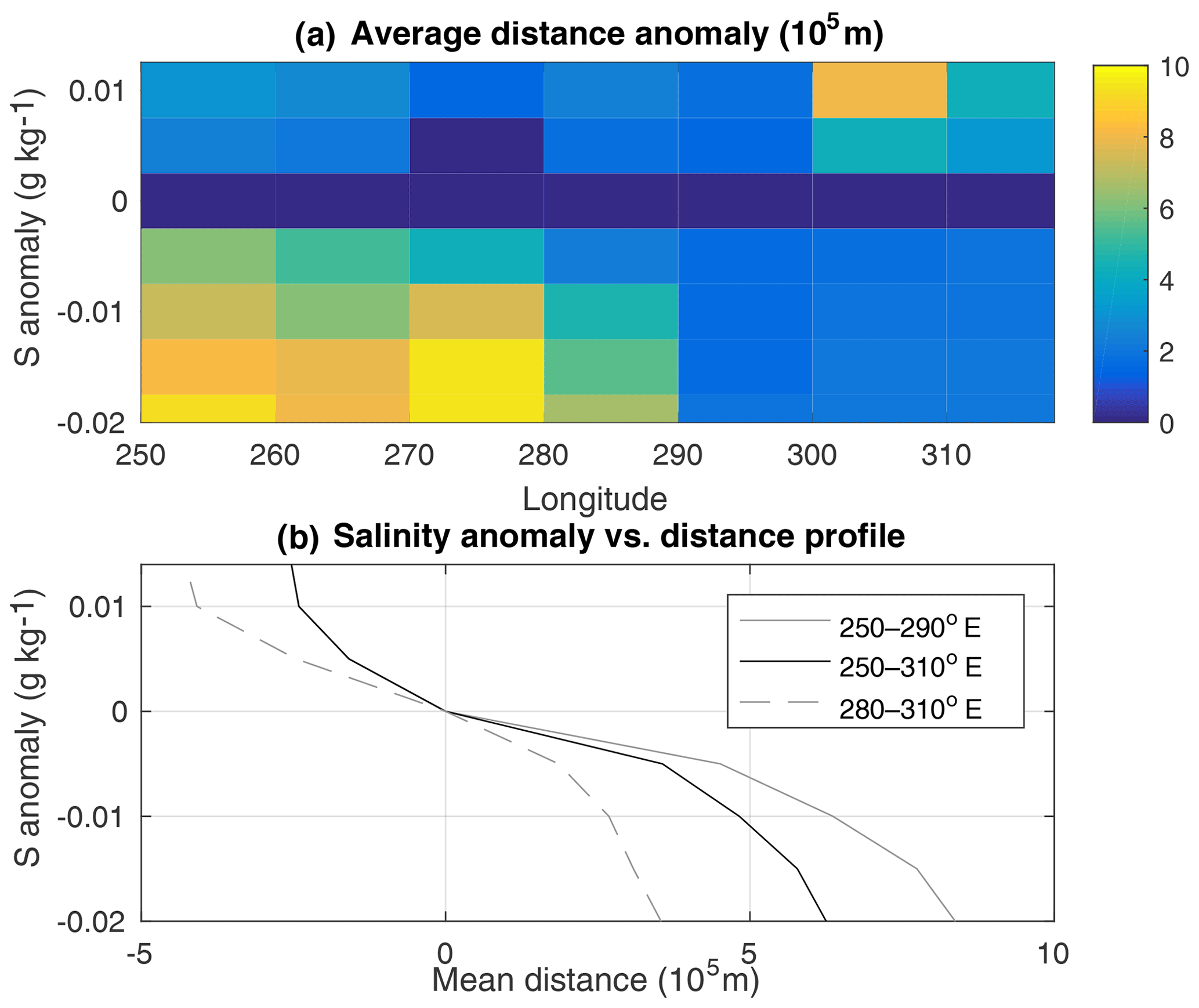
Figure 7(a) The mean minimum distance of observations in each salinity class to the black line in 10^∘ longitude bands. (b) The mean salinity-versus-distance profile for the entire survey region and for a western and an eastern region. In the westernmost region there were insufficient high-salinity observations to produce a profile for the positive salinity anomalies there.

Download

Given distance as a function of salinity for each section, $\stackrel{\mathrm{‾}}{D\left(S^{\prime }\right)}$, we use the climatological hydrography to map the tracer from isopycnal salinity-anomaly to distance-anomaly coordinates. The same distance-versus-salinity-anomaly profiles are used on all isopycnals.

We apply a non-linear least-squares fit of a two-dimensional Gaussian distribution to each section to yield the standard width in the isopycnal direction (σ_iso), with the resulting along-isopycnal component of the second moments shown in Fig. 8 now in the conventional units of squared metres.

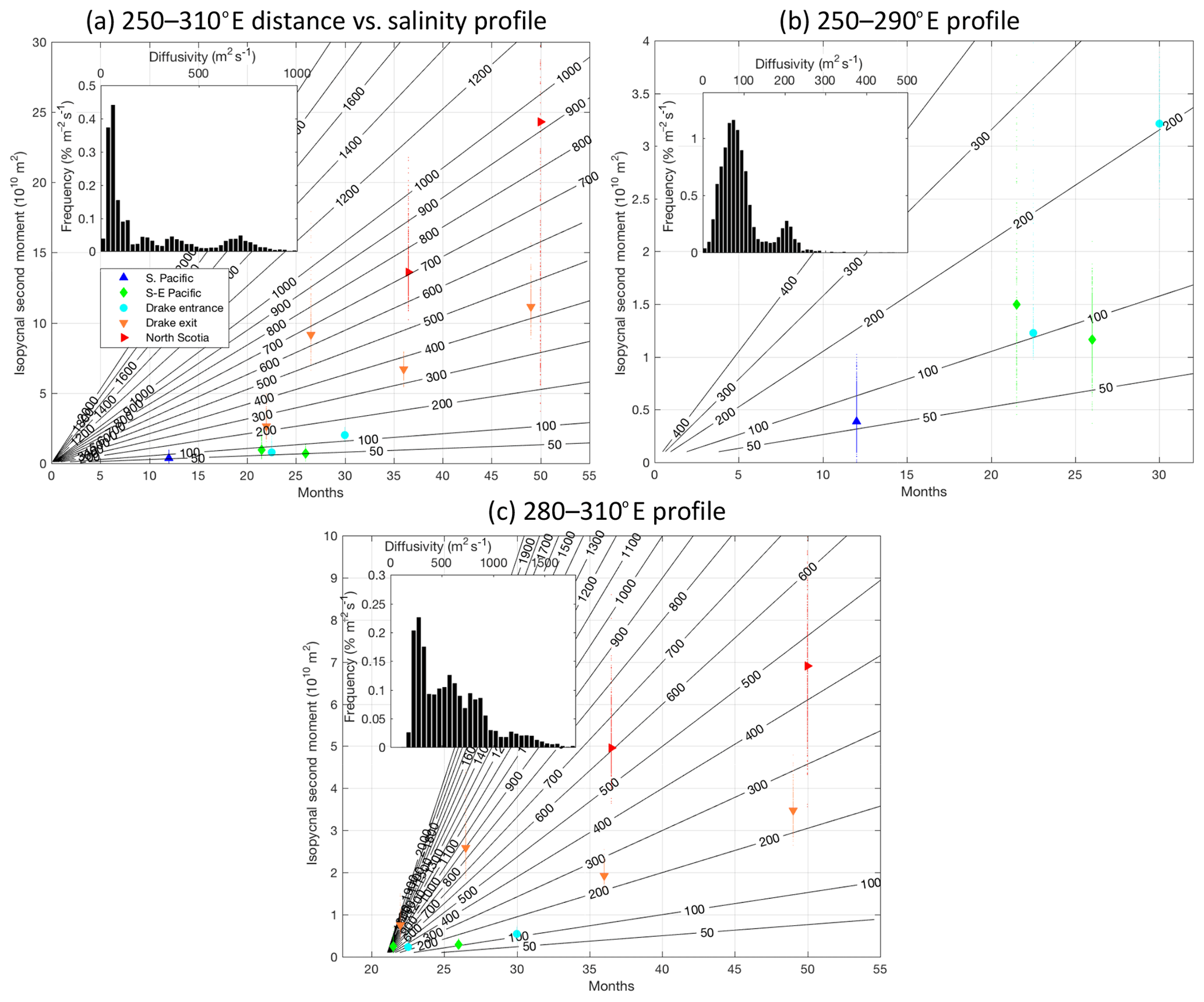
Figure 8Isopycnal second moment of the tracer versus time since release, computed by projecting from tracer versus salinity anomaly into tracer versus distance, using a constant distance-versus-salinity profile. Panel (a) uses the profile from salinity data between 250 and 310^∘ E, (b) between 250 and 290^∘ E, and (c) 280 and 310^∘ E. Only tracer data gathered between those longitudes are shown. Each small marker represents a single member of the bootstrap ensemble and the larger marker the result of using all the data. The rate of change of the second moment in time is proportional to an apparent diffusivity (Eq. 1). Contours of apparent diffusivity are shown in black. Panels (a) and (b) show the case where the growth is linear from the release date, and (c) shows an offset of 21 months. Within each panel are shown the distribution functions of diffusivity estimates. In (a) and (b) these assume constant mixing from the release date. In (c) these estimates are based on the slope between the two eastern South Pacific sections and the two Scotia Sea sections.

Download

Given the change in the isopycnal second moment at each section ($\mathrm{\Delta }{\mathit{\sigma }}_{\mathrm{iso}}^{\mathrm{2}}$) and the time between section occupations (Δt), we can examine whether the tracer patch grows linearly, as would be expected from the ensemble area of a tracer patch with a constant diffusion coefficient (K_iso), such that

or if there is a temporal change in the growth rate either indicating different phases of the tracer evolution or geographical changes in K_iso.

In Fig. 8a, the second moments of the tracer are plotted as a function of time since release, using the mean salinity-versus-distance profile for the entire survey region. The classical calculation of the eddy diffusion coefficient based on Lagrangian data statistics was first introduced by Taylor (1922), who showed that under stationary conditions and after multiples of the Lagrangian correlation time, the area of a cloud of particles will grow linearly in time at a rate known as the effective eddy diffusivity. In this paper, we describe the linear growth from an infinitesimally small second moment with an “apparent diffusivity”. We next test this simple model of the growth of the tracer patch.

The apparent diffusivity is on the order of 50 m² s⁻¹ in the South Pacific leading up to the eastern South Pacific and Drake Entry sections and on the order of 400 m² s⁻¹ integrated over both the South Pacific and Scotia Sea regions. Downstream sections such as the Drake exit exhibit a large range of apparent diffusivities (i.e. when fitting second-moment growth all the way back to the origin) from the order of 200 m² s⁻¹ to the order of 600 m² s⁻¹, with later diffusivities tending to be larger even though the tracer has transited through the same geographical domain.

The change in apparent diffusivity between the earlier period and the western region and the later period and the eastern region, can be explained by at least three mechanisms: first, the difference in salinity gradient from the eastern to western region could translate into a virtual increase in apparent diffusivity as we have not yet accounted for such variations; second, the tracer may enter a region of more vigorous isopycnal mixing in the east; third, the apparent diffusivity is low at the early stage after tracer release because the tracer is still growing slowly as it forms filaments, before achieving faster growth after some lag time on the order of months to years (Garrett, 1983) and coincidentally when it enters the eastern region. The later two possibilities are addressed in more detail in the discussion section below.

To ascertain whether the change in apparent diffusivity could be explained by a change in the salinity gradient itself, we estimate a diffusivity in two phases using salinity-versus-distance profiles for the western and eastern regions separately (shown in Fig. 7). For the western region, we use only tracer measurements made in the first 26 months of the experiment and to the west of 290^∘ E. These estimates assume that mixing is linear from the release date. For the eastern region, we use only measurements made after 20 months and to the east of 280^∘ E. The eastern region estimates are made by taking the difference in the second-moment estimates from the south-east Pacific and Drake Entry sections and those measured at least 6 months later at the Drake exit and North Scotia sections. Although the statistics of the diffusivity estimates are not normal, we estimate the error bounds based on the 16th and 84th deciles (equivalent to ±1 standard deviation for a normal distribution).

Considering only the sections in the western region in the first 26 months, this analysis yields a diffusivity of 40–100 m² s⁻¹ (45–130 m² s⁻¹ if the final Drake Entry section at 30 months is included). We estimate a diffusivity of 250–870 m² s⁻¹ in the eastern region. This suggests that even when considering a change in the background salinity gradient there is still a substantial increase in diffusivity between the western and eastern region, so something else must explain this increase in diffusivity.

In a previous study, data from DIMES together with output of a numerical model were used to quantify isopycnal mixing in the eastern South Pacific (Tulloch et al., 2014). Those authors estimated a diffusion coefficient using the ensemble area of the tracer patch and found it to be of the order of 700 m² s⁻¹. An additional study used float observations to estimate a diffusion coefficient on the order of 800 m² s⁻¹ (LaCasce et al., 2014). Here, we have taken a complementary approach and attempt to quantify the irreversible mixing of the tracer as it spreads both in the South Pacific and Scotia Sea regions. Using our novel coordinate framework and assuming linear growth from an infinitesimally small patch, we demonstrate that, as the tracer disperses, the evolution of the area of the tracer is consistent with an apparent diffusivity of 70±30 m² s⁻¹ in the south-east Pacific, increasing to 560±310 m² s⁻¹ downstream as the tracer enters the Scotia Sea. While our estimate of apparent diffusivity in the Scotia Sea is consistent with Tulloch et al. (2014) and LaCasce et al. (2014), we note that our estimate in the south-east Pacific is significantly lower than their estimate.

While we cannot here disentangle the exact reason for such a difference with previous authors for our estimate in the south-east Pacific, we explore whether the increase in dispersion from the south-east Pacific to the Scotia Sea could be explained by the time evolution of the regime of dispersion of the tracer patch rather than by a regional difference in conditions. In other words, we explore the possibility that the tracer dispersion is initially very slow and rapidly increases after some time lag, making a linear growth assumption like we did above inappropriate. Indeed, Garrett (1983) discussed that the evolution of a tracer patch (that has already formed an approximately Gaussian distribution; the DIMES tracer was initially dispersed in a 20 km by 20 km cross shape) should have two distinct phases in its evolution: one first phase where the tracer forms streaks, so where the actual area of the tracer grows slowly; and a second phase after some time lag as the actual area approaches the area of an ellipse surrounding the tracer; the growth rate of the actual area of the tracer then asymptotes toward linear growth.

The time lag and time evolution of the area of the tracer patch in the two different regimes can be expressed as a function of a number of parameters of the flow field (Garrett, 1983, see the Appendix). By trying to best estimate those parameters and bootstrapping a best fit to our observed tracer patch dispersion with the Garrett (1983) theoretical prediction, we are able to estimate the isopycnal mixing K_iso reached in the phase of linear growth of the tracer patch, as well as the time lag at which this regime is reached (see the Appendix). From the ensemble of solutions, we find that the isopycnal diffusivity lies between 240 and 550 m² s⁻¹ (Fig. A1a shows the distribution). The lag times are between 20 and 32 months. If we use the much lower small-scale diffusivity (K_s=0.04 m² s⁻¹; see Appendix), the solutions for K_iso and the lag time do not change substantially (K_iso=290–600 m² s⁻¹; lag time =19–29 months). Both the results of Tulloch et al. (2014) and LaCasce et al. (2014) are consistent with the linear growth rate that we find here of 240–550 m² s⁻¹. This linear growth sets in after an initial slow growth phase, as predicted by the theory of Garrett (1983) and suggested by our observation of a step change in diffusivities between the South Pacific and Scotia Sea. Additionally the lag time is consistent with the point at which we note the change in diffusivities.

Above we are not arguing that there is necessarily a large increase in effective isopycnal stirring between the Pacific and Atlantic in the Southern Ocean. We are pointing out that an increase in the rate of irreversible mixing of a tracer patch, as our analysis suggests, is expected (Garrett, 1983) even without changes in rates of eddy stirring or small-scale mixing.

Alternative explanations for the spread of apparent isopycnal diffusivities in Fig. 8 cannot be ruled out. It is possible that frontal suppression inhibited mixing in the South Pacific and that this broke down as the tracer entered Drake Passage, although this interpretation would arguably be at odds with the diffusivity estimates made by Tulloch et al. (2014) and LaCasce et al. (2014). Alternatively, the tracer growth may not have reached the lag time and may still be in a relatively weak mixing regime (potentially explaining why the implied diffusivities are on the low side of Tulloch et al. (2014) and LaCasce et al. (2014)). In this case, it may be that geographical changes in vertical mixing drive geographical changes in the size of filaments and therefore the apparent isopycnal mixing inferred (Smith and Ferrari, 2009). Vertical mixing was indeed found to increase as the tracer moved from the Pacific Ocean into the Scotia Sea (Watson et al., 2013).

We have neglected the effects of along-stream mixing in this analysis as is customary in vertical mixing calculations (Ledwell et al., 1993). In principle, if the tracer is mixed at the same rate in the along-stream direction at all salinities, the maximum concentration of the tracer will reduce but the second moment will be preserved. If, however, the tracer is mixed at different rates at different salinities (for example, it is mixed strongly close to the release salinity and weakly further away), then this could distort the second moment and therefore affect our diffusivity estimates.

The data are publicly available through the British Oceanographic Data Centre (http://www.bodc.ac.uk/projects/data_management/international/dimes/, last access: 9 March 2020).

Author contributions, based on the CRediT model, were as follows: JDZ contributed to conceptualisation, formal analysis, investigation, methodology, validation, visualisation, writing as well as the original draft and writing along with review and editing; JBS contributed to conceptualisation, data curation, investigation, methodology, resources, software and writing as well as review and editing; AJSM contributed to conceptualisation, data curation, investigation, methodology, resources, software and writing as well as review and editing; ACNG contributed to funding acquisition, investigation, methodology, resources and writing as well as review and editing; AJW contributed to data curation, funding acquisition, investigation, methodology, resources, software and writing as well as review and editing; MJM contributed to data curation, funding acquisition, investigation, writing, and review and editing; BAK contributed to data curation, funding acquisition, methodology and software.

The authors declare that they have no conflict of interest.

This research has been supported by the Natural Environment Research Council (grant no. NE/E006000/1).

This paper was edited by Ilker Fer and reviewed by two anonymous referees.