the Creative Commons Attribution 4.0 License.
the Creative Commons Attribution 4.0 License.
 | 17 Mar 2020
Impact of tidal dynamics on diel vertical migration of zooplankton in Hudson Bay
Vladislav Y. Petrusevich
Igor A. Dmitrenko
Andrea Niemi
Sergey A. Kirillov
Christina Michelle Kamula
Zou Zou A. Kuzyk
David G. Barber
Jens K. Ehn
Hudson Bay is a large seasonally ice-covered Canadian inland sea connected to the Arctic Ocean and North Atlantic through Foxe Basin and Hudson Strait. This study investigates zooplankton distribution, dynamics, and factors controlling them during open-water and ice cover periods (from September 2016 to October 2017) in Hudson Bay. A mooring equipped with two acoustic Doppler current profilers (ADCPs) and a sediment trap was deployed in September 2016 in Hudson Bay ∼190 km northeast from the port of Churchill. The backscatter intensity and vertical velocity time series showed a pattern typical for zooplankton diel vertical migration (DVM). The sediment trap collected five zooplankton taxa including two calanoid copepods (Calanus glacialis and Pseudocalanus spp.), a pelagic sea snail (Limacina helicina), a gelatinous arrow worm (Parasagitta elegans), and an amphipod (Themisto libellula). From the acquired acoustic data we observed the interaction of DVM with multiple factors including lunar light, tides, and water and sea ice dynamics. Solar illuminance was the major factor determining migration pattern, but unlike at some other polar and subpolar regions, moonlight had little effect on DVM, while tidal dynamics are important. The presented data constitute the first-ever observed DVM in Hudson Bay during winter and its interaction with the tidal dynamics.


The diel vertical migration (DVM) of zooplankton is a synchronized movement of individuals through the water column and is considered to be the largest daily synchronized migration of biomass in the ocean (Brierley, 2014). This migration is majorly controlled by two biological factors: (1) predator avoidance by staying away from the illuminated surface layer during the day and thus reducing the light-dependent mortality risk (Hays, 2003; Ringelberg, 2010; Torgersen, 2003) and (2) optimization of feeding, with the assumption that algal biomass is greater in the surface layer during evening hours and zooplankton rise to feed on it in the evening (Lampert, 1989). There are three general DVM patterns: (1) the most common one is nocturnal when zooplankton ascend around sunset and remain at upper depths during the night, descending around sunrise and remaining at depth during the day (Cisewski et al., 2010; Cohen and Forward, 2002). (2) Then there is a reverse pattern when zooplankton ascend at dawn and descend at dusk (Heywood, 1996; Pascual et al., 2017). And finally, (3) there is a twilight DVM pattern when zooplankton ascend at sunset, descend around midnight, ascend again, and finally descend at sunset (Cohen and Forward, 2005; Valle-Levinson et al., 2014). This pattern is sometimes called midnight sink. DVM of zooplankton is an important process of the carbon and nitrogen cycle in marine systems because it effectively acts as a biological pump, transporting carbon and nitrogen vertically below the mixed layer by respiration and excretion (Darnis et al., 2017; Doney and Steinberg, 2013; Falk-Petersen et al., 2008). The following research question needs to be addressed: what sets the timing of this synchronized movement in the Arctic environment? Earlier studies of DVM in the Arctic were focused on the period of midnight sun or the transition period from midnight sun to a day–night cycle (Blachowiak-Samolyk et al., 2006; Cottier et al., 2006; Falk-Petersen et al., 2008; Fortier et al., 2001; Kosobokova, 1978; Rabindranath et al., 2010). Recent studies based on acoustic backscatter data and zooplankton sampling showed the presence of synchronized DVM behavior continuing throughout the Arctic winter, during both open and ice-covered waters (Båtnes et al., 2015; Benoit et al., 2010; Berge et al., 2009, 2012, 2015a, b; Cohen et al., 2015; Last et al., 2016; Petrusevich et al., 2016; Wallace et al., 2010). It was proposed that (Berge et al., 2014; Hobbs et al., 2018; Last et al., 2016; Petrusevich et al., 2016), during polar night, DVM is regulated by diel variations in solar and lunar illumination, which are at intensities far below the threshold of human perception. Another reason for increasing interest in studying DVM patterns in various geophysical and geographical environments and their seasonal changes in response to changing oceanographic conditions is that they could help inform us about physical oceanographic processes. Furthermore, DVM patterns can be significantly modified by water column stratification (Berge et al., 2014) and water dynamics, such as polynya-induced estuarine-like circulation (Petrusevich et al., 2016), tidal currents (Hill, 1991, 1994; Valle-Levinson et al., 2014), and upwelling and downwelling (Dmitrenko et al., 2019; Wang et al., 2015).
In the Arctic Ocean, the DVM process can be difficult to measure. However, there has been recent success in using data obtained by an acoustic Doppler current profiler (ADCP), which is a modern oceanographic instrument commonly used to measure the vertical profile of current velocities. Because the velocity profiling by an ADCP is based on processing the measured intensity of acoustic pings backscattered by suspended particles in the water column, further processing of the measured acoustic backscatter to volume backscatter strength (Deines, 1999) has been successful in quantifying zooplankton abundance (Bozzano et al., 2014; Brierley et al., 2006; Cisewski et al., 2010; Cisewski and Strass, 2016; Fielding et al., 2004; Guerra et al., 2019; Hobbs et al., 2018; Last et al., 2016; Lemon et al., 2008; Petrusevich et al., 2016; Potiris et al., 2018, etc.). ADCP backscatter data, validated using a time series of zooplankton samples collected from sediment traps, provide a particularly useful tool for better understanding the effects of physical oceanographic processes on zooplankton DVM, changes in zooplankton community composition throughout the year, and marine ecosystem function and carbon cycling (Berge et al., 2009; Willis et al., 2006, 2008).
In this study, we are focused on zooplankton organisms with sizes from 500 µm and up. This group of zooplankton is primarily detected by ADCP backscatter (Cisewski and Strass, 2016; Pinot and Jansá, 2001) and allows for comparison with previous studies on zooplankton caught by sediment traps (see Forbes et al., 1992; Pospelova et al., 2010).
In this study, factors controlling zooplankton distribution during the open-water and ice-covered periods are investigated using ADCP data together with sediment trap samples for the first time in Hudson Bay. The main objectives are to (1) examine DVM during open-water and ice-covered seasons in Hudson Bay in 2016–2017, (2) identify zooplankton species involved in DVM, and (3) describe the DVM response to solar and lunar light, tides, and water and sea ice dynamics.
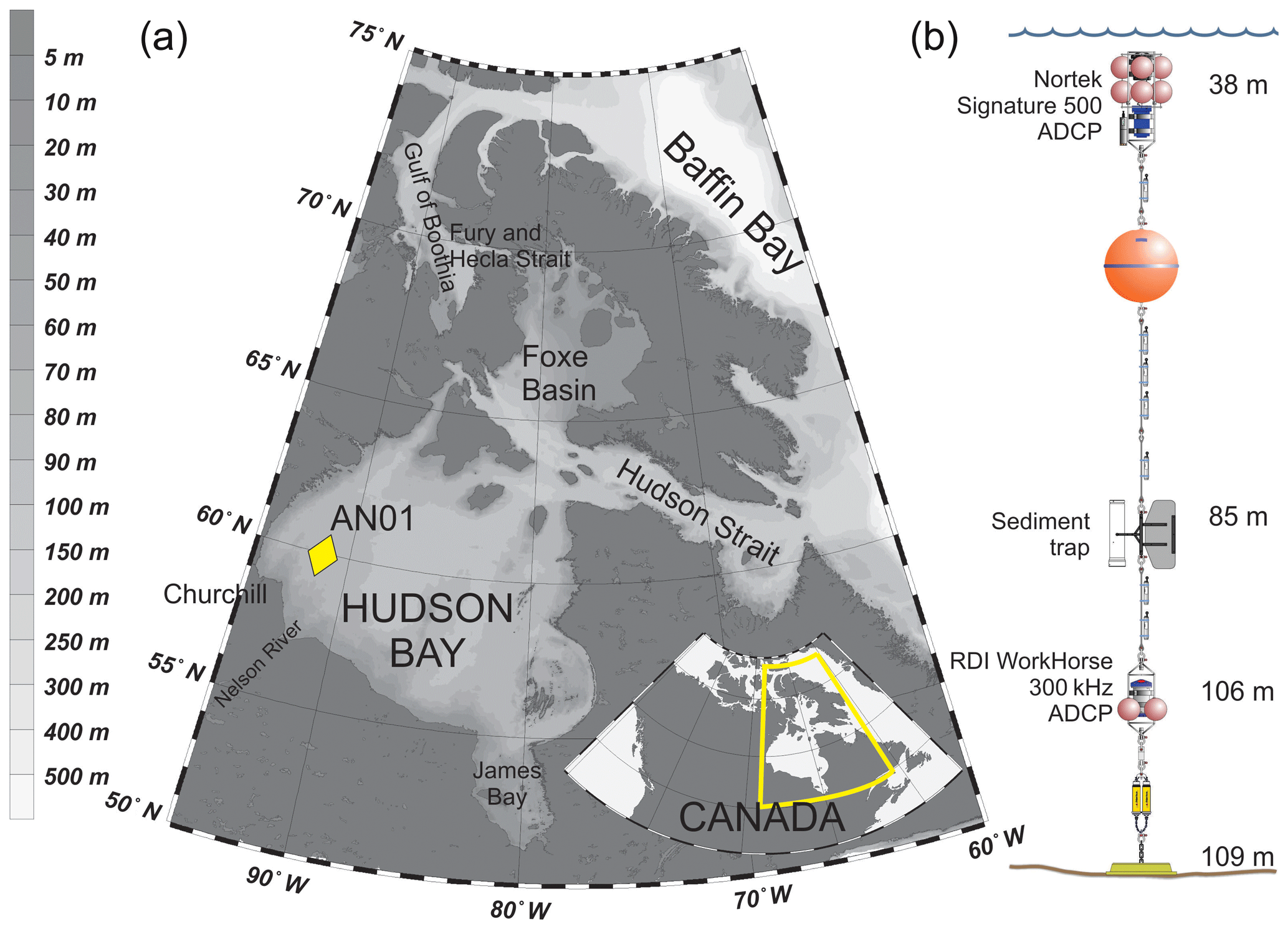
Figure 1(a) A bathymetric map of the Hudson Bay region and the location of the mooring (AN01). The inset map shows Hudson Bay on a map of Canada. (b) Schematic illustration of the mooring AN01 setup.
Hudson Bay (Fig. 1a) is a large (with an area about 831 000 km2) seasonally ice-covered shallow inland sea with an average depth of 125 m and maximum depth below 300 m (Burt et al., 2016; Ingram and Prinseberg, 1998; Macdonald and Kuzyk, 2011; Petrusevich et al., 2018; St-Laurent et al., 2008; Straneo and Saucier, 2008). The seabed is characterized by fluted tills, postglacial infills, moraines, and subglacial channels eroded to bedrock, resulting in bottom depth varying from 200 m to ∼10 m (Josenhans and Zevenhuizen, 1990). The tides are mostly lunar semidiurnal (M2) with an amplitude of about 3 m at the entrance to Hudson Bay from Hudson Strait (Prinsenberg and Freeman, 1986; St-Laurent et al., 2008) and about 1.5 m in Churchill (Prinsenberg, 1987; Saucier et al., 2004; Ray, 2016) (Fig. 1). The marine water masses flow into Hudson Bay through two gateways: (1) the Gulf of Boothia to Fury and Hecla Strait through Foxe Basin and (2) Baffin Bay to Hudson Strait (Fig. 1a). Measurements of alkalinity and nutrient ratios suggest that the water masses within Hudson Bay are dominated by Pacific-origin waters from the Arctic Ocean (Burt et al., 2016; Jones et al., 2003), and the phytoplankton and zooplankton assemblages resemble those in the Arctic Ocean (Estrada et al., 2012; Runge and Ingram, 1991). Freshwater inputs to Hudson Bay are very large, including river runoff from the largest watershed in Canada, together with seasonal inputs of sea ice melt. The freshwater inputs together produce strong stratification at the surface in summer (Ferland et al., 2011). Fall storms and cooling, followed by brine rejection from sea ice formation during winter produces a winter surface mixed layer varying from ∼40 to >90 m deep throughout Hudson Bay (Prinsenberg, 1987; Saucier et al., 2004).
Hudson Bay is ice-covered during 7–9 months a year, with ice formation typically starting in the northwest part of the bay in late October (Hochheim and Barber, 2014). The mean maximum ice thickness ranges from 1.2 m in the northwest to 1.7 m in the east (Landy et al., 2017). Around Churchill, the ice usually starts forming in October–November and breaks up in May–June (Gagnon and Gough, 2005, 2006). Since 1996 the open-water season has, on average, increased by 3.1 (±0.6) weeks in Hudson Bay, with mean shifts in dates for freeze-up and breakup of 1.6 (±0.3) and 1.5 (±0.4) weeks accordingly (Hochheim and Barber, 2014).
There have been few studies on zooplankton community composition in Hudson Bay. Among the macrozooplankton species found in Hudson Bay, Parasagitta elegans is the most abundant species, followed by Aglantha digitale as the second most abundant (Estrada et al., 2012). The mesoplankton community in Hudson Bay is dominated by small copepods: Oithona similis, Oncaea borealis, and Microcalanus (Estrada et al., 2012). Zooplankton diversity is generally low at high latitudes (Conover and Huntley, 1991). Typically, salinity gradients and freshwater discharge play an important role in determining species diversity (Witman et al., 2008). Seasonality in food availability is another significant challenging factor for zooplankton in high latitudes (Bandara et al., 2016; Carmack and Wassmann, 2006; Varpe, 2012).
3.1 Mooring configuration and setup
A bottom-anchored oceanographic mooring (Fig. 1b) was deployed at 109 m of depth ∼190 km northeast from the port of Churchill (59∘58.156′ N 91∘57.144′ W) on 26 September 2016 and recovered on 30 October 2017. The mooring setup consisted of (i) one upward-looking five-beam Signature 500 ADCP by Nortek placed at 38 m of depth, (ii) an upward-looking four-beam 300 kHz Workhorse Sentinel ADCP by RD Instruments placed at 106 m of depth, and (iii) one Gurney Instruments “Baker-type” sequential sediment trap (Baker and Milburn, 1983) at 85 m with a collection area of 0.032 m2. Several conductivity–temperature, conductivity–temperature–turbidity, and temperature–turbidity sensors were also deployed at various depths on the mooring, but the data obtained by these sensors were not analyzed in this study.
The velocity and acoustic backscatter (ABS) intensity were measured by a Teledyne RD Instruments (RDI) ADCP between 8 and 100 m at 2 m depth intervals, with a 15 min ensemble time interval and 15 pings per ensemble. The ADCP velocity measurement precision and resolution were ±0.5 % and ±0.1 cm s−1, respectively. The accuracy of the ADCP vertical velocity measurements are not validated; however, the RDI reports that the vertical velocity is more accurate, by at least a factor of 2, than the horizontal velocity (Wood and Gartner, 2010). The compass accuracy was ±2∘, and compass readings were corrected by adding magnetic declination.
The sediment trap was programmed to start a collection at 4 October 2016 at 00:00 CST with intervals of 35 d for each vial collected. Prior to boarding the vessel, sediment trap preservative density solution was prepared at the Churchill Northern Studies Centre (CNSC). To prepare the solution, 10 L of seawater was collected from the Churchill port wharf and filtered through 0.7 µm Whatman GF/F filters. The salinity of the filtered seawater was adjusted from 26.7 to 37 psu with 88.065 g of ultraclean sea salt. Borax (44.4 g) was slowly added to 0.45 L of 37 % formaldehyde, placed on a magnetic stir plate overnight to dissolve, and decanted into 8.55 L of filtered seawater. Approximately 1 h before deployment of the sediment traps, pre-acid-cleaned vials were placed inside the preprogrammed sampling carrousel and filled to the surface with the preservative solution. The trap was assembled and kept upright prior to and during deployment. During deployment, the different species of zooplankton were captured by the sediment trap (Fig. 6).
3.2 Data collection and post-processing
ADCPs, unlike echo sounders (Lemon et al., 2012, 2001), are limited in deriving accurate quantitative estimates of biomass due to calibration difficulties because their acoustic beams are narrow and inclined from the vertical (Brierley et al., 1998; Lemon et al., 2008; Sato et al., 2013; Vestheim et al., 2014). But with the application of beam geometry correction, ADCPs are commonly used for qualitative studies, as they can provide information on zooplankton presence and behavior (Hobbs et al., 2018; Last et al., 2016; Petrusevich et al., 2016). To correct for the ADCP beam geometry, we derived the volume backscatter strength (VBS) Sv in decibels (dB) from echo intensity following the procedure described by Deines (1999). The issue of acoustic signal scattering by bubbles, waves, and sea ice was addressed by removing the top 8 m readings from all backscatter and velocity data.
The total sky illumination for day and night was modeled using the skylight.m function
from the astronomy package for MATLAB (Ofek, 2014) and a
simple exponential decay radiative transfer model for estimating under-ice
illumination (Grenfell and
Maykut, 1977; Perovich, 1996). Transmittance through the sea ice was
calculated following Eq. (1):
where α is the surface albedo, κt is the bulk extinction coefficient of the sea ice cover, and z is the ice thickness. The values of the coefficients used in the exponential decay model were adjusted for the first-year sea ice: α=0.8 and κt=1.2. We did not have any data for snow cover available, so the presence of snow cover was omitted in the transmittance model. However, an albedo of 0.8 was used to simulate the high albedo at visible wavelengths for snow-covered or white ice surfaces.
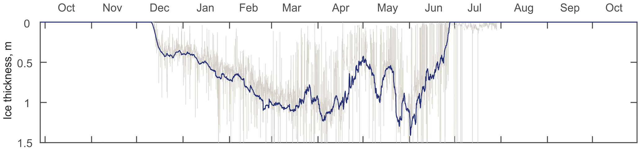
Figure 2ADCP-measured ice thickness at the mooring location (AN01) during winter 2016–2017. Gray and blue lines represent the filtered and daily averaged ice thicknesses, respectively.
The thickness of (Fig. 2) ice at the mooring location was estimated from the ice draft evaluated from the distance to the ice–ocean interface measured by the Nortek ADCP (Banks et al., 2006; Björk et al., 2008; Shcherbina et al., 2005; Visbeck and Fischer, 1995). The draft was further transformed to the ice thickness by multiplying by a factor of 1.115 for the density difference between seawater and sea ice (Bourke and Paquette, 1989). The acoustic-derived thicknesses were corrected for ADCP tilt, sea surface height, atmospheric pressure (Krishfield et al., 2014), and the speed of sound. The extreme outliers were excluded, and the mean daily ice thicknesses were calculated for further analysis (Fig. 2).
The Environment and Climate Change Canada weather station at Churchill airport (YYQ), located ∼190 km southwest from the mooring location, provided wind data for most of the time of mooring deployment, except for the period of 27 March–7 April 2017. The daily mean wind speed magnitude was used to compile the wind speed time series (Fig. 3c).
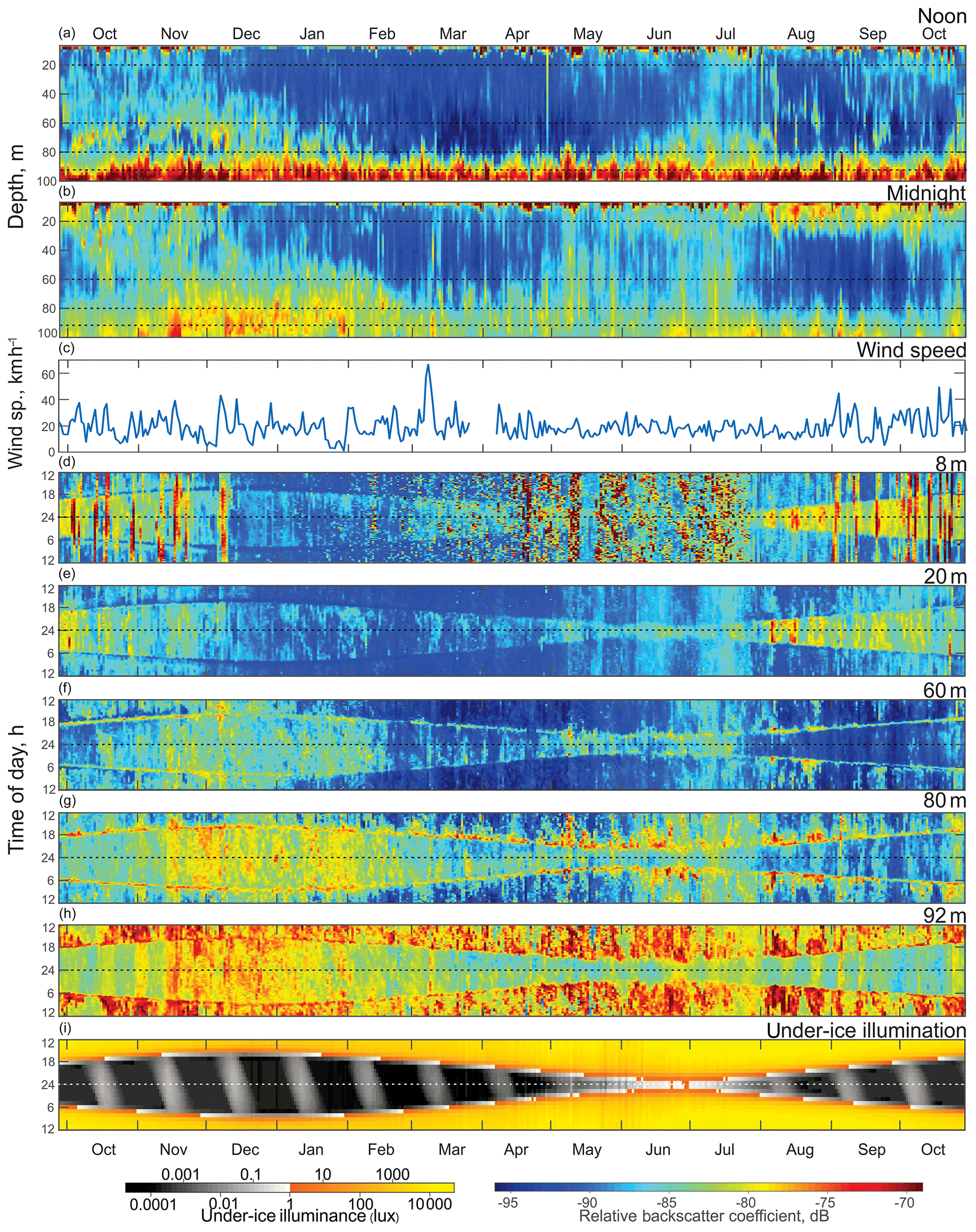
Figure 3Time series (October 2016 to October 2017) of the (a) ADCP acoustic volume backscatter coefficient at noon and (b) at midnight, (c) daily mean wind speed measured at Churchill airport (YYQ), and (d)–(i) actograms of ADCP acoustic backscatter at five depth levels: (d) 8 m, (e) 20 m, (f) 60 m, (g) 80 m, and (h) 92 m, as well as (i) modeled under-ice illuminance. Dashed horizontal lines represent astronomical midnight. The diurnal signal is presented at the vertical axis, while the long-term changes in diurnal behavior are presented along the horizontal axis.
On recovery of the mooring, sediment trap samples were photographed, poured into acid-cleaned 250 mL amber glass bottles, and stored in the dark at approximately 4 ∘C during transport to the Centre for Earth Observation Science, University of Manitoba. Samples were poured through a 500 µm NITEX mesh sieve to separate the larger zooplankton fraction. The 500 µm mesh was selected to maintain consistency and allow for comparison with previous studies (see Forbes et al., 1992; Pospelova et al., 2010). Because of this, smaller species, nauplii, eggs, and fecal pellets were largely missed from the >500 µm fraction. However, the >500 µm organisms represent the group of zooplankton primarily detected as ADCP backscatter (Cisewski and Strass, 2016; Pinot and Jansá, 2001). Zooplankton taxonomy identification was conducted at the Freshwater Institute (DFO) to the lowest taxonomic level possible, enumerated, and measured. The entire sample was scanned for large and rare organisms and then the sample was split, with a Motoda box splitter, and a minimum of 300 organisms were counted for each sample.
4.1 Ice thickness and under-ice illumination
At the mooring location, the ice started rapidly forming in the second week of December. By mid-December the thickness reached 0.4 m and gradually grew until the middle of March up to 1 m (Fig. 2). Afterwards, the ice thickness at the mooring location varied due to seasonal factors, e.g., polynyas, sea ice melting, etc.
Modeled under-ice illumination time series, as well as the volume backscatter strength and vertical velocity time series, were presented in the form of actograms (Figs. 3d–g and 4). An actogram, being a common method of data display in chronobiological research, has recently been used for displaying zooplankton DVM (Hobbs et al., 2018; Last et al., 2016; Petrusevich et al., 2016; Tran et al., 2016).
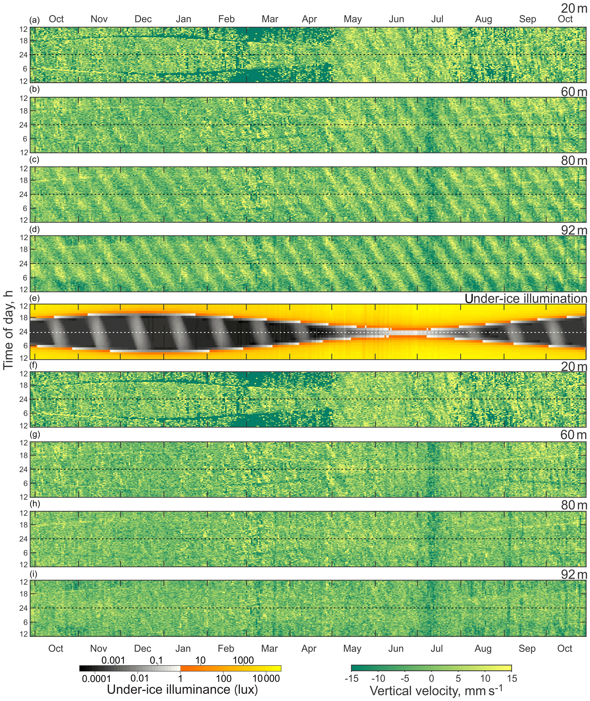
Figure 4Actograms of (a–d) ADCP-measured vertical velocity (mm s−1) at four depth levels: (a) 20 m, (b) 60 m, (c) 80 m, and (d) 92 m. (e) Modeled under-ice illuminance and (f–i) residual vertical velocity (mm s−1, tidal signal subtracted) at four depth levels: (f) 20 m, (g) 60 m, (h) 80 m, and (i) 92 m. Positive and negative values correspond to the upward and downward net flux. Dashed horizontal lines represent astronomical midnight.
The actogram of the modeled under-ice illumination (Figs. 3i and 4e) shows continuous daily maximums at noon, with minimum values of 2000 lx around the winter solstice and maximum values of 10 000 lx in the middle of summer. Maximum under-ice lunar illumination was around 0.1 lx during a full moon under sea ice about 0.5 m thick.
4.2 Volume backscatter strength (VBS)
To analyze the depth-dependent behavior of scatterers involved in diurnal vertical migration, we computed the volume backscatter strength (VBS) time series at noon (Fig. 3a) and at midnight (Fig. 3b). The mean difference between noontime and midnight VBS was dB at the 96–100 m depth layer and at the 10–28 m layer. Running an F-statistic test returned statistical significance with 95 % confidence for the VBS difference below 58 m and above 48 m. Noontime series show persistent maximum backscatter strength near the bottom below 92 m of depth, which is consistent with DVM. Some scatter stayed at noon at the 60–80 m layer during October–January and at 70–80 m in June–July.
The near-bottom maximum for the midnight time series of VBS is significantly lower compared to that for noon. Midnight time series during October–February and May–July showed a wider spread of scatterers over the depth. During winter months (December–February), the thickness of this layer of midnight bottom scatterers gradually decreased with the growth of sea ice. There are periods of higher VBS at the bottom layer with the same periodicity of 14 d as the superposition maxima of the M2 and S2 tidal components (spring tide) throughout the whole time series. There was a seasonal variation of these periodic VBS maxima: they increased during summer–fall and decreased in winter. It should be noted that during November–January there were higher values of backscatter below 80 m of depth.
VBS was calculated for depths of 8, 20, 60, 80, and 92 m and is shown as actograms in Fig. 3d–h. Overall, VBS actograms show a similar shape as that of the under-ice solar illumination actogram (Fig. 3i). This resemblance in shape is outlined by reduced VBS at 8 and 20 m actograms (Fig. 3d–e) and enhanced at 60, 80, and 92 m actograms (Fig. 3f–h) during dawn and dusk. Reduced under-ice illumination from December to March corresponded with reduced VBS through the whole water column, followed by increased illumination during ice breakup and open-water periods (April to October) and an increase in VBS within all five depth bins. Like the noon and midnight VBS time series, there is a relatively higher signal at 60, 80, and 92 m of depth in November–January during the night.
The VBS actograms (Fig. 3d–h) show the presence of vertical bands of higher VBS with 14 d periodicity at multiple depths. In the upper 8 and 20 m (Fig. 3d–e), these bands spread through the night period, while at 80 and 92 m actograms the bands spread throughout the whole day, with different values of VBS during the day and night. In the 8 m actogram (Fig. 3d) there are also nonperiodic bands of high backscatter that span from 1 to 5 d in duration. These bands spread throughout the whole day and correspond to the periods of wind speed increasing to strong wind, gale, and storm values (30 km h−1 and up) during the ice-free season (Fig. 3c).
Figure 3c shows daily mean wind speed measured at Churchill airport (YYQ). There were several observed periods of mean wind speed higher than 30 km h−1, which corresponds to strong wind (37–61 km h−1) and gale (62–87 km h−1) wind speed values, with maximum wind gusting up to 77 km h−1. Normally these storm events lasted from 1 to 6 d.
4.3 Vertical velocity actograms
The vertical velocity actograms were calculated for the same depths as VBS actograms (Fig. 4a–d). Positive velocities are associated with the upward movement of particles. The seasonal shape of vertical velocity actograms is similar to the shape of under-ice illumination (Figs. 3c and 4e) and VBS actograms (Fig. 3d–g). The change in vertical speed associated with spring tide is present on the vertical velocity actograms in the form of slanted strips of 14 d periodicity, with amplitude increasing with depth and reaching maximum values in the range of 10–15 mm s−1.
The vertical velocity actograms were post-processed (Fig. 4f–i) to remove the semidiurnal tidal components (M2 and S2) from the vertical velocity data, which would otherwise create a tidal background signal in the form of slanted strips of 14 d periodicity on the actograms (Fig. 4a–d). A tidal harmonic analysis was performed for the vertical velocity time series using T_Tide toolbox for MATLAB (Pawlowicz et al., 2002). There was a small distinguishable diurnal variation of vertical velocity in the 20 and 60 m actograms (Fig. 4f and g) during the period of the full moon in October, November, and December resembling the slanted shape of lunar illumination on the under-ice illumination actogram (Fig. 4e).
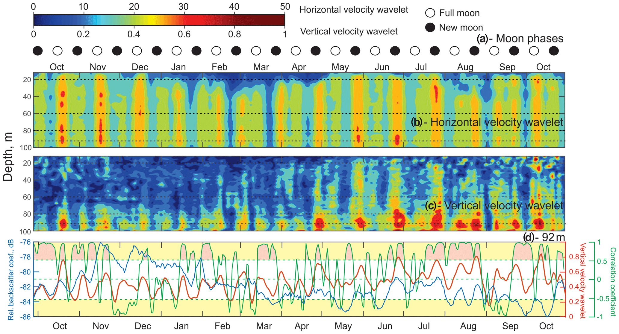
Figure 5Time series of (a) lunar phases for 2016–2017. ◦: Full moon. •: New moon. (b, c) The absolute value of the wavelet power spectrum for the time series of horizontal velocity (b) and vertical velocity (c) computed for the semidiurnal frequency band (12 h) as a function of depth. (d) The correlation coefficient (green line) between time series of VBS (blue line) and the vertical velocity wavelet (red line) at 92 m of depth. Yellow shading identifies the correlation coefficient levels exceeding ±0.53, which are statistically significant for the 95 % confidence level. Pink shading identifies the events during which this statistically significant correlation was observed.
4.4 Wavelet analysis
Time series of the wavelet power spectrum for the semidiurnal tidal currents were computed to account for their spring–neap and seasonal variability. Wavelets for horizontal and vertical velocities (Fig. 5b and c) show absolute maximum values during spring tides, which is consistent with the full moon and new moon phases (Fig. 5a). The power spectrum range for horizontal velocities was in general over 1 order of magnitude higher than for vertical velocity, which is consistent with the fact that horizontal tidal currents tend to be at least an order of magnitude larger than vertical ones. There is a spatial difference between the horizontal and vertical velocity power spectrum. The horizontal velocity wavelet has maximums that spread through the whole water column during the ice-free season and below 30 m of depth in the presence of ice cover (December–April). The vertical velocity spectrum during October–April has maximums mostly concentrated below 70 m of depth. There is a seasonal variation for the vertical velocity wavelet, with May–June wavelet maximums starting to spread through the whole water column.
For the analysis of ADCP-measured current velocities, we used wavelet transformation to derive the time-dependent behavior of horizontal and vertical current velocities at the semidiurnal tidal frequency band that dominates the backscatter spectrum. In this study, we used the generalized Morse wavelet (with parameters β=100 and γ=3) and jWavelet toolbox (part of jLab toolbox) for signal processing (Lilly, 2017, 2019; Lilly and Gascard, 2006; Lilly and Olhede, 2009).
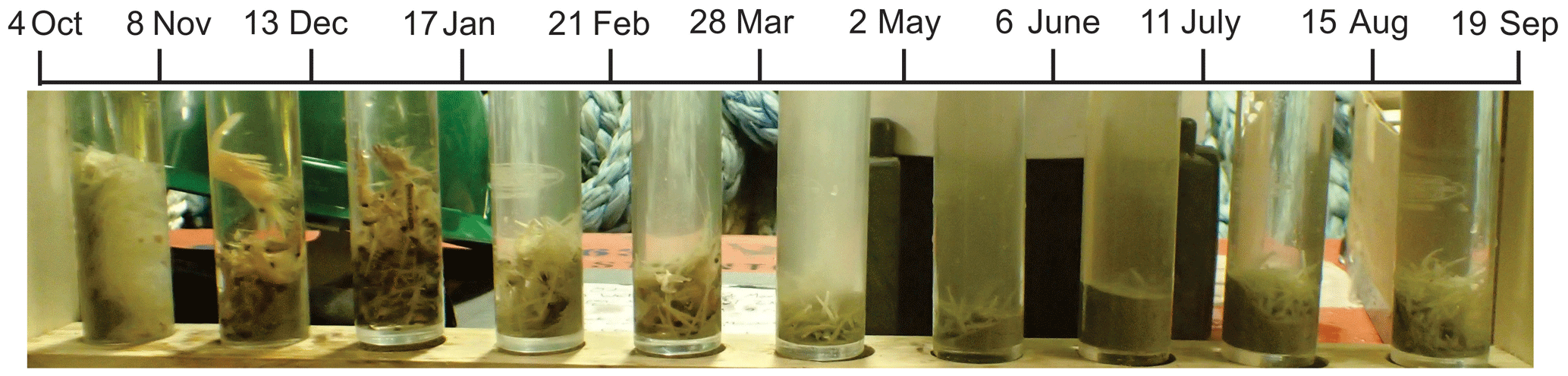
4.5 Sediment trap zooplankton
Zooplankton >500 µm captured in the sediment trap samples (Fig. 6) were dominated (>98 %) by five taxa including two calanoid copepods (Calanus glacialis and Pseudocalanus spp.), a pelagic sea snail (Limacina helicina), a gelatinous arrow worm (Parasagitta elegans), and an amphipod (Themisto libellula) (Table 1, Fig. 7). The abundance of organisms in the trap was generally lowest from March to July with the exception of juvenile (2 mm length) T. libellula in bottle 6.
Table 1Abundance () and length (mm) of the dominant zooplankton (>500 µm) in each bottle of the sediment trap at AN01 from October 2016 to August 2017. Note: T. libellula juveniles and adults are presented separately for bottle 6; adult abundance and length are in parentheses.
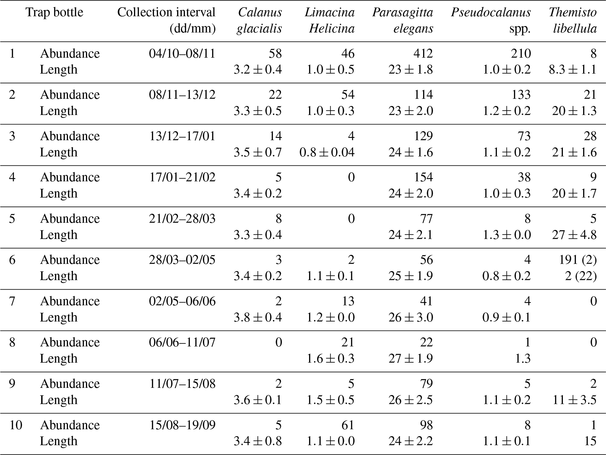
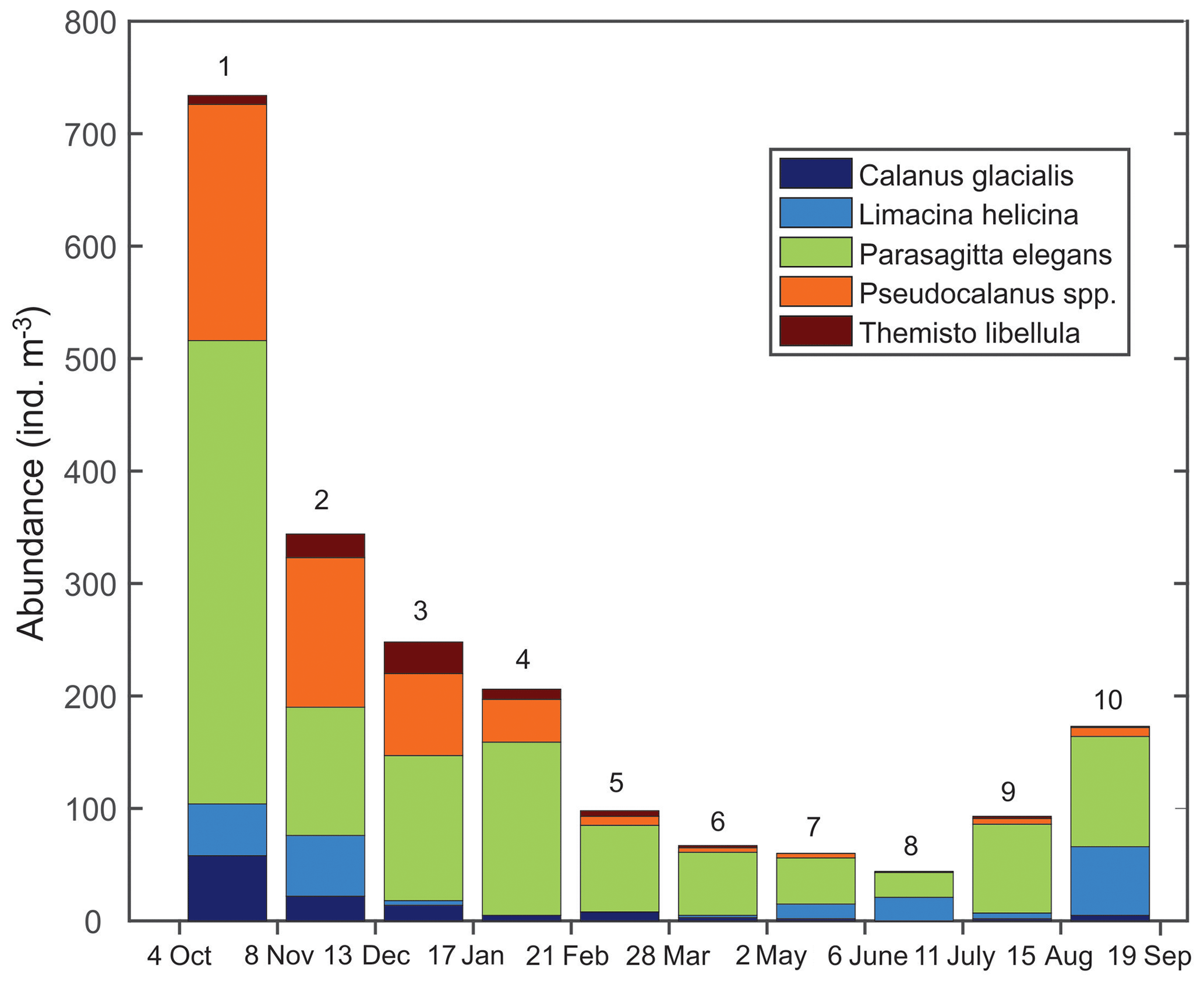
Figure 7Abundance () of the dominant zooplankton (>500 µm) in each bottle of the sediment trap at AN01 from October 2016 to August 2017.
5.1 Zooplankton species associated with DVM in Hudson Bay
The presence of seasonal ice cover acts as a barrier to using traditional zooplankton sampling techniques. But using both moored and ice-tethered ADCPs in high latitudes has been successful for studying zooplankton presence, behavior, and particularly DVM patterns (Darnis et al., 2017; Hobbs et al., 2018; Petrusevich et al., 2016; Wallace et al., 2010). Even though acoustic backscatter from the single-frequency ADCP does not provide any information on the identity of zooplankton species involved in DVM, signal strength can provide an indication of zooplankton presence provided there is information on the zooplankton species. Sound is effectively scattered by objects of the size of the wavelength. For 300 kHz ADCP, it is about 5 mm. It is known that zooplankton species with a body size less than the wavelength by an order of magnitude (in our case 0.5–5 mm) are capable of creating strong backscatter when there is a sufficient abundance of them in the water column (Cisewski and Strass, 2016; Pinot and Jansá, 2001). The backscatter strength of zooplankton species also depends on their acoustic properties, such as shape, internal structure, orientation in the water column, and body composition, which causes a difference between the speed of sound in their bodies and the surrounding seawater (Stanton et al., 1994, 1998a, b). For example, the species with hard shells (like Limacina helicina) and gaseous enclosures scatter sound stronger than gelatinous ones (Lavery et al., 2007; Warren and Wiebe, 2008). It should be mentioned that 300 kHz ADCP can be effectively used for suspended sediment transport monitoring (Venditti et al., 2016), but here are some general considerations that need to be taken into account: 300 kHz ADCPs are used for suspended sediment monitoring, mostly in rivers with high sediment loads (hundreds of milligrams per liter). Our mooring was located ∼190 km northeast from the Churchill River, which does not create a significant plume of sediment into the system. The mooring turbidity sensor located at 41 m of depth did not record values higher than 34 FTU, which corresponds to TSS of ∼30 mg L−1, with an average turbidity of 7 FTU; this corresponds to TSS ∼5 mg L−1. At 100 m of depth, we do not expect high levels of sediment from resuspension. Also taking into consideration the fact that sound is effectively scattered by objects of the size of the wavelength and that the mean particle size detected by 300 kHz ADCP is in the range of 0.5 to 5 mm (Jourdin et al., 2014), sporadic smaller scatterers, like sediment and phytoplankton, can effectively be eliminated as potential scatterers. This allows us to consider zooplankton to be the main scatterers in our case.
Fish also can be detected with the ADCP used. It should be noted though that large mesopelagic fishes are rare in the Canadian Arctic (Berge et al., 2015b). Arctic cod (Boreogadus saida) is the dominant pelagic fish in the Canadian Arctic (e.g., Benoit et al., 2008; LeBlanc et al., 2019), and therefore the acoustic signals related to fish are generally assumed to be only Arctic cod. The distribution of Arctic cod is known for regions such as the Beaufort Sea (Geoffroy et al., 2016) and Baffin Bay (LeBlanc et al., 2019). However, there is little known for Hudson Bay. It is expected that Hudson Bay Arctic cod behave similarly, with adult aggregations near the bottom in deep waters and young (year 1–2) and larval stages in surface aggregations. The young cod are ice-associated during the winter period, i.e., no migration to depth. As such, any backscatter associated with near-surface young cod would have been removed as part of the removal of the top 8 m of backscatter during post-processing. Arctic cod do not school. So, its presence in the proximity of the mooring will be more sporadic, and acoustic backscatter will be significantly less than the backscatter from much more abundant zooplankton.
The trap samples reflect the presence of >500 µm zooplankton in the water column during the annual cycle. However, the absence of a species from the trap samples (e.g., L. helicina in January–March) does not confirm its absence from the water column. The most abundant species from the zooplankton trap catch (Parasagitta elegans, Pseudocalanus, and L. helicina) had lengths of 20–30, 0.6–1.4, and 0.4–2 mm, respectively. Less abundant species from the trap (Calanus glacialis and Themisto libellula) had lengths of 2.8–4.2 and 7.2–31.8 mm, respectively. P. elegans and T. libellula lengths are in the range of ADCP wavelength and should thus effectively act as scatterers. Lengths of C. glacialis, Pseudocalanus, and L. helicina are less than the wavelength by an order of magnitude. However, their abundance in the water column during the open-water season (Estrada et al., 2012) is high enough (>1000 ind m3) to expect a backscatter signal. L. helicina's hard shell should be another contributing factor to backscatter strength. Therefore, we assume that all the species identified in the sediment trap could act as acoustic scatterers contributing to the VBS signal analyzed in this study.
The zooplankton caught in our sediment trap provide general information on the zooplankton community composition and its change over the course of the year near the mooring location. Sediment trap samples may not quantitatively reflect zooplankton composition in the water column due to species-specific collection efficiencies. Comparisons between net and trap samples from Franklin Bay indicate that the abundance of L. helicina and some species of copepods could be estimated from sediment traps, whereas the abundance of other key species, such as C. hyperboreus, could not be accurately estimated from sediment trap samples (Makabe et al., 2016).
The ADCP analysis indicates that zooplankton in Hudson Bay undergo both seasonal and diel migration. This is similar to measured seasonal migration by copepod species in the southern Arctic Ocean and in Rijpfjorden in Svalbard (Falk-Petersen et al., 2008). Seasonal migration is occurring in Hudson Bay despite shallower overwintering waters than in Svalbard and the Beaufort Sea. The observed diel migration in Hudson Bay is similar to other Arctic locations (Berge et al., 2014, 2015b; Hobbs et al., 2018; Last et al., 2016; Petrusevich et al., 2016), suggesting that DVM is an important consideration for carbon–nitrogen transfer within the relatively shallow Hudson Bay system.
Zooplankton species identified from the sediment trap suggest that multiple species could be involved in the DVM. The identification of individual species involved in DVM is not currently possible and is challenged by issues such as the overlapping of signals. Comparison between acoustic and net data in Kongsfjorden, Svalbard, led to the conclusion that the acoustic backscatter signal from numerically dominant Calanus copepods is typically overwhelmed by the signal from larger and less abundant zooplankton species, such as Themisto (Berge et al., 2014). Large copepods (like Calanus spp.) and chaetognaths (P. elegans) were observed performing diel migrations in Kongsfjorden (Darnis et al., 2017). While our sediment trap showed the prevalence of gelatinous zooplankton species (Fig. 7 – P. elegans), the detection of their migration by ADCP backscattering could be underestimated because gelatinous species are weak scatterers.
Regardless, there is a pump of carbon–nitrogen occurring within Hudson Bay based on zooplankton DVM, and seasonal differences (discussed in the next section) could impact this vertical transport of elements. The collected acoustic data at hand are not valid to quantify zooplankton biomass involved in DVM. However, we can use them to document and better understand important aspects of DVM, such as links between its seasonal cycle and the dynamics of sea ice cover and under-ice illuminance, as well as the effects of windstorms and tides on DVM patterns.
5.2 DVM seasonal cycle, sea ice cover, and under-ice illuminance
The mooring site is located 6∘ south of the Arctic Circle and polar twilight zone. Hudson Bay is located more south than other seasonally sea-ice-covered Arctic and sub-Arctic regions where DVM was observed. In those locations, DVM during the winter was primarily controlled by twilight and the lunar light (Last et al., 2016; Petrusevich et al., 2016). In this study, DVM was generally controlled by solar illumination throughout the whole year, which is evident from the shape of the VBS (Fig. 3d–h) and vertical velocity actograms (Fig. 4). The actograms are nearly symmetric around astronomic midnight (dashed horizontal line, Figs. 3 and 4) and the winter and summer solstice. During dawn and dusk, there was reduced VBS on the 8 and 20 m actograms (Fig. 3d–e) and enhanced VBS on the 60, 80, and 92 m actograms (Fig. 3f–h). These dawn and dusk absences and enhancements can be interpreted as an indication of zooplankton swimming behavior during these periods, following a nocturnal DVM pattern. The increased backscatter at dawn and dusk on the 60 and 80 m actograms was observed regardless of the presence of ice cover.
The noontime VBS time series showed consistent maximum backscatter strength below 92 m of depth (Fig. 3a). Compared to the midnight time series (Fig. 3b), it is clear that the backscatter was associated with DVM rather than sediment resuspension caused by the lunar semidiurnal M2 tide with a period of 12 h 25 min. The midnight VBS time series (Fig. 3b) and VBS actograms (Fig. 3d–h) confirm that the zooplankton were aggregated in the upper water column at midnight, likely feeding.
Seasonal variations in zooplankton migration and distribution in the water column were observed throughout the entire time series. The sediment trap at 85 m of depth may have captured zooplankton species migrating vertically and possibly also individuals sinking to the bottom (Fig. 6). The strong VBS of −70 dB during noon at the 90–100 m depth layer (Fig. 3a), compared with −80 dB at midnight (Fig. 3b), suggests that noontime DVM-associated zooplankton biomass was primarily located at the bottom layer through the annual cycle. From October to the middle of January, however, there was a layer of VBS in the range of −80 to −75 dB at 60–80 m of depth, which can be interpreted as some of the zooplankton staying at that depth instead of migrating all the way down to the bottom for daytime or to the surface at night. The 60–80 m aggregation of zooplankton from October to January corresponds to the first three sampling bottles of the sediment trap when the highest abundance of zooplankton was observed with the abundance of dominant species per 35 d sampling period, decreasing from 720 down to 250 (Fig. 7). From the middle of January to early May, most of the zooplankton biomass at midnight did not migrate above 60 m of depth. From May to July zooplankton returned to the vertical migration pattern observed when zooplankton remain near the bottom at noon and migrate to the surface at night. In July, some zooplankton stayed in the surface layer at noon. This corresponds to the beginning of the ice-free season (Fig. 2) when long periods of daylight and the abundance of phytoplankton disrupts DVM. Once the sea ice was completely gone in early August, there was a change in zooplankton distribution in the water column. During midnight, some zooplankton remained at the bottom, while others migrated to the surface layer, likely feeding during the short night and moving back down to the bottom for the light time. This suggests that different zooplankton scatter species and/or size classes are responding differently to both solar cues and ice cover.
In certain cases vertical velocity actograms can be used to estimate swimming direction and velocity (Petrusevich et al., 2016), for example when actograms are averaged for layers several meters deep for the estimation of swimming direction and when individual profiles are averaged over a period of a few days for velocity estimation. This method works well when there is no tidal signal to be subtracted from the vertical velocity data; otherwise, it makes computation rather complicated.
5.3 Masking of DVM signal in the upper layer by storms
The 8 m depth actogram (Fig. 3d) shows several bands of higher VBS of different durations that are not observed at the deeper layers. These bands spread throughout the entire 24 h day for a duration of one to several days. These bands (Fig. 3d) nicely correspond to daily mean wind speed exceeding 25 km h−1 (Fig. 3c) during most of the ice-free season (October–mid December 2016 and September–October 2017). Irregular spots of higher VBS can be related to the bubbling generated by the wind forcing. In contrast, during the ice-covered season, periods of high winds were not associated with higher VBS. For example, on 7–10 March 2017, the daily mean wind was 66 km h−1, but there were no bands of higher VBS on the 8 m actogram (Fig. 3d), indicating that ice cover partly protected the water column from wind stress. Irregular spots of higher VBS (Fig. 3d) during the ice-covered period (February–March) could be attributed to frazil ice formation. With the onset of spring melt (May–July), there is also more noise-type VBS that could be attributed to the release of ice-rafted sediment during the melting of the sea ice. The large amount of sediment present in the May–July sediment trap bottles (Fig. 6) provides proof for the presence of sinking sediment during this period.
An alternative explanation of higher VBS at 8 m of depth is a different feeding pattern for nonvisual predators like chaetognaths (including P. elegans). While mature species are known to perform DVM, in some cases juvenile individuals were found near the surface during the daytime (Brodeur and Terazaki, 1999).
5.4 Disruption of DVM by the spring tide
Time series of the wavelet power spectrum for horizontal and vertical velocities (Fig. 5b, c) show absolute maximum values during spring tides, which correspond to full moon and new moon phases (Fig. 5a). For the 92 m depth, the 14 d running correlation (Fig. 5d, green line) between midnight VBS (blue line) and the vertical velocity wavelet (red line) was calculated. Correlations exceeding ±0.53 are statistically significant at the 95 % confidence level (Fig. 5d, yellow shading). Pink shading identifies events during which this statistically significant positive correlation was observed. Negative correlations are artificial and have no physical meaning. The periods of low correlation were from the end of November to mid-January, mid-February to mid-March, April to mid-June, and the first half of September. A statistically significant positive correlation suggests a relationship between VBS and tidal forcing.
In the presence of background stratification, the barotropic tide interacts with sloping bottom topography in the proximity of the mooring location (Fig. 1), which is typical for Hudson Bay (Petrusevich et al., 2018). This interaction generates the vertical divergence and convergence of tidal flow, resulting in the depth-dependent behavior of the vertical velocity at a tidal frequency defined here as the baroclinic tide. The seasonal character of the baroclinic tide can also be affected by density stratification. During May–October 2017 the vertical velocity wavelet maximums were amplified (Fig. 5c). During this period there were DVM disruptions throughout the water column that are clearly evident on VBS actograms (Fig. 3d–g) and noon VBS time series (Fig. 3a).
Zooplankton normally avoid expending additional energy to cross such an interface, which is a horizontal interface with a strong velocity gradient, thereby resulting in a weakened or absent a DVM signal (Petrusevich et al., 2016). Similar observations of disrupted zooplankton vertical migration have been linked to upwelling and downwelling events (Dmitrenko et al., 2019). The same considerations can be applied to this study when water dynamics are impacted by vertical currents generated by baroclinic tides and enhanced during spring tide. During spring tide, zooplankton showed a weakened DVM to avoid moving against the vertically diverging and converging tidal flow, as follows from the VBS actograms. This disruption can be moon-controlled as reported by Hobbs et al. (2018), Last et al. (2016), and Petrusevich et al. (2016). However, in this study, the lunar origin of this disruption is attributed to tidal dynamics rather than moonlight because disruptions occurred during the full moon and new moon phases.
A 1-year-long acoustic backscatter and vertical velocity time series, obtained using a 300 kHz ADCP on a mooring deployed from September 2016 to October 2017 in southeast Hudson Bay (∼190 km northeast from the port of Churchill), revealed a distinct diurnal pattern consistent with zooplankton diel vertical migration (DVM).
In this study, we were able to determine the presence of multiple zooplankton species that could have been involved in DVM from samples collected by the sediment trap. The sediment trap was programmed to collect settling material over a complete annual cycle (35 d interval and averaging period), and consequently the collection was not timed to shorter tidal cycles. This limited the identification of specific species whose DVM was detected by the 300 kHz ADCP and altered by M2 tidal water dynamics. Using shorter sediment trap time intervals and/or the in situ sampling required for the identification of the zooplankton species involved in DVM will be incorporated in future mooring deployments.
The major factors determining the observed DVM pattern were as follows.
-
Illuminance. Unlike other ice-covered and ice-free Arctic and sub-Arctic locations such as Svalbard and northeast Greenland (Last et al., 2016; Petrusevich et al., 2016), DVM in Hudson Bay is controlled by solar illumination throughout the whole year, not by moonlight.
-
Tidal dynamics. The tide in Hudson Bay is mostly lunar semidiurnal (M2) with an amplitude of a few meters. The area in the proximity of the mooring has variable bottom topography (Fig. 1). The barotropic tide interacts with bottom topography, generating tidal flow diverging and converging vertically. It seems that zooplankton tend to avoid expending additional energy swimming against the vertical flow. This response of zooplankton is consistent with the zooplankton tendency to stay away from the layers with enhanced water dynamics and to adjust their DVM accordingly.
-
Storm-induced disruptions. When daily mean wind speed exceeded 25 km h−1 during most of the ice-free season in the surface layer, there were observed irregular spots of higher VBS related to the bubbling generated by the wind forcing.
The backscatter and velocity data are archived in the Centre for Earth Observation Science (University of Manitoba) and are restricted for open access in accordance with University of Manitoba policy for 2 years after observations are completed. The MATLAB code used for data processing is available from Vladislav Y. Petrusevich upon request.
VYP prepared the paper with contributions from all coauthors (IAD, AN, SAK, CMK, ZZAK, DGB, and JKE). VYP, SAK, and CMK deployed and retrieved the mooring in Hudson Bay. AN processed and presented zooplankton data from the sediment trap. VYP processed and presented acoustic data from the ADCP. SAK processed and provided data for the ice draft.
The authors declare that they have no conflict of interest.
This article is part of the special issue “Developments in the science and history of tides (OS/ACP/HGSS/NPG/SE inter-journal SI)”. It is not associated with a conference.
We would like to give special thanks to Alexis Burt of Fisheries and Oceans Canada for processing zooplankton taxa. We would like to thank Captain Neil J. MacDonald, Chief Officer Kevin Jones, the crew of the CCGS Henry Larsen, the Canadian Coast Guard, technician Sylvan Blondeau of Laval University, and Christopher Peck of the University of Manitoba for their assistance with successful mooring retrieval, as well Nathalie Thériault for coordinating BaySys field logistics.
This research has been supported by the Natural Sciences and Engineering Council of Canada (NSERC) Collaborative Research and Development project: BaySys (grant no. CRDPJ 470028‐14). Funding for this work, including field studies, was provided by NSERC, Manitoba Hydro, the Canada Excellence Research Chair (CERC) program, and the Canada Research Chairs (CRC) program.
This paper was edited by Mattias Green and reviewed by three anonymous referees.
Baker, E. T. and Milburn, H. B.: An instrument system for the investigation of particle fluxes, Cont. Shelf Res., 1, 425–435, https://doi.org/10.1016/0278-4343(83)90006-7, 1983.
Bandara, K., Varpe, Ø., J. E. S., Wallenschus, J., Berge, J., and Eiane, K.: Seasonal vertical strategies in a high-Arctic coastal zooplankton community, Mar. Ecol. Prog. Ser., 555, 49–64, https://doi.org/10.3354/meps11831, 2016.
Banks, C. J., Brandon, M. A., and Garthwaite, P. H.: Measurement of Sea-ice draft using upward-looking ADCP on an autonomous underwater vehicle, Ann. Glaciol., 44, 211–216, https://doi.org/10.3189/172756406781811871, 2006.
Båtnes, A. S., Miljeteig, C., Berge, J., Greenacre, M., and Johnsen, G.: Quantifying the light sensitivity of Calanus spp. during the polar night: potential for orchestrated migrations conducted by ambient light from the sun, moon, or aurora borealis?, Polar Biol., 38, 51–65, https://doi.org/10.1007/s00300-013-1415-4, 2015.
Benoit, D., Simard, Y., and Fortier, L.: Hydroacoustic detection of large winter aggregations of Arctic cod (Boreogadus saida) at depth in ice-covered Franklin Bay (Beaufort Sea), J. Geophys. Res., 113, C06S90, https://doi.org/10.1029/2007JC004276, 2008.
Benoit, D., Simard, Y., Gagné, J., Geoffroy, M., and Fortier, L.: From polar night to midnight sun: photoperiod, seal predation, and the diel vertical migrations of polar cod (Boreogadus saida) under landfast ice in the Arctic Ocean, Polar Biol., 33, 1505–1520, https://doi.org/10.1007/s00300-010-0840-x, 2010.
Berge, J., Cottier, F., Last, K. S., Varpe, Ø., Leu, E., Søreide, J., Eiane, K., Falk-Petersen, S., Willis, K., Nygård, H., Vogedes, D., Griffiths, C., Johnsen, G., Lorentzen, D., and Brierley, A. S.: Diel vertical migration of Arctic zooplankton during the polar night, Biol. Lett., 5, 69–72, https://doi.org/10.1098/rsbl.2008.0484, 2009.
Berge, J., Båtnes, A. S., Johnsen, G., Blackwell, S. M., and Moline, M. A.: Bioluminescence in the high Arctic during the polar night, Mar. Biol., 159, 231–237, https://doi.org/10.1007/s00227-011-1798-0, 2012.
Berge, J., Cottier, F., Varpe, O., Renaud, P. E., Falk-Petersen, S., Kwasniewski, S., Griffiths, C., Søreide, J. E., Johnsen, G., Aubert, A., Bjærke, O., Hovinen, J., Jung-Madsen, S., Tveit, M., and Majaneva, S.: Arctic complexity: a case study on diel vertical migration of zooplankton., J. Plankton Res., 36, 1279–1297, https://doi.org/10.1093/plankt/fbu059, 2014.
Berge, J., Daase, M., Renaud, P. E., Ambrose, W. G., Darnis, G., Last, K. S., Leu, E., Cohen, J. H., Johnsen, G., Moline, M. A., Cottier, F., Varpe, Ø., Shunatova, N., Bałazy, P., Morata, N., Massabuau, J.-C., Falk-Petersen, S., Kosobokova, K., Hoppe, C. J. M., Węsławski, J. M., Kukliński, P., Legeżyńska, J., Nikishina, D., Cusa, M., Kędra, M., Włodarska-Kowalczuk, M., Vogedes, D., Camus, L., Tran, D., Michaud, E., Gabrielsen, T. M., Granovitch, A., Gonchar, A., Krapp, R., and Callesen, T. A.: Unexpected Levels of Biological Activity during the Polar Night Offer New Perspectives on a Warming Arctic, Curr. Biol., 25, 2555–2561, https://doi.org/10.1016/j.cub.2015.08.024, 2015b.
Berge, J., Renaud, P. E., Darnis, G., Cottier, F., Last, K., Gabrielsen, T. M., Johnsen, G., Seuthe, L., Weslawski, J. M., Leu, E., Moline, M., Nahrgang, J., Søreide, J. E., Varpe, Ø., Lønne, O. J., Daase, M., and Falk-Petersen, S.: In the dark: A review of ecosystem processes during the Arctic polar night, Prog. Oceanogr., 139, 258–271, https://doi.org/10.1016/j.pocean.2015.08.005, 2015a.
Björk, G., Nohr, C., Gustafsson, B. G., and Lindberg, A. E. B.: Ice dynamics in the Bothnian Bay inferred from ADCP measurements, Tellus A, 60, 178–188, https://doi.org/10.1111/j.1600-0870.2007.00282.x, 2008.
Blachowiak-Samolyk, K., Kwasniewski, S., Richardson, K., Dmoch, K., Hansen, E., Hop, H., Falk-Petersen, S., and Mouritsen, L. T.: Arctic zooplankton do not perform diel vertical migration (DVM) during periods of midnight sun, Mar. Ecol. Prog. Ser., 308, 101–116, https://doi.org/10.3354/meps308101, 2006.
Bourke, R. H. and Paquette, R. G.: Estimating the thickness of sea ice, J. Geophys. Res.-Ocean., 94, 919–923, https://doi.org/10.1029/JC094iC01p00919, 1989.
Bozzano, R., Fanelli, E., Pensieri, S., Picco, P., and Schiano, M. E.: Temporal variations of zooplankton biomass in the Ligurian Sea inferred from long time series of ADCP data, Ocean Sci., 10, 93–105, https://doi.org/10.5194/os-10-93-2014, 2014.
Brierley, A. S.: Diel vertical migration, Curr. Biol., 24, R1074–R1076, https://doi.org/10.1016/j.cub.2014.08.054, 2014.
Brierley, A. S., Brandon, M. A., and Watkins, J. L.: An assessment of the utility of an acoustic Doppler current profiler for biomass estimation, Deep-Sea Res. Pt. I, 45, 1555–1573, https://doi.org/10.1016/S0967-0637(98)00012-0, 1998.
Brierley, A. S., Saunders, R. A., Bone, D. G., Murphy, E. J., Enderlein, P., Conti, S. G., and Demer, D. A.: Use of moored acoustic instruments to measure short-term variability in abundance of Antarctic krill, Limnol. Oceanogr. Methods, 4, 18–29, https://doi.org/10.4319/lom.2006.4.18, 2006.
Brodeur, R. D. and Terazaki, M.: Springtime abundance of chaetognaths in the shelf region of the northern Gulf of Alaska, with observations on the vertical distribution and feeding of Sagitta elegans, Fish. Oceanogr., 8, 93–103, https://doi.org/10.1046/j.1365-2419.1999.00099.x, 1999.
Burt, W. J., Thomas, H., Miller, L. A., Granskog, M. A., Papakyriakou, T. N., and Pengelly, L.: Inorganic carbon cycling and biogeochemical processes in an Arctic inland sea (Hudson Bay), Biogeosciences, 13, 4659–4671, https://doi.org/10.5194/bg-13-4659-2016, 2016.
Carmack, E. and Wassmann, P.: Food webs and physical-biological coupling on pan-Arctic shelves: Unifying concepts and comprehensive perspectives, Prog. Oceanogr., 71, 446–477, https://doi.org/10.1016/j.pocean.2006.10.004, 2006.
Cisewski, B. and Strass, V. H.: Acoustic insights into the zooplankton dynamics of the eastern Weddell Sea, Prog. Oceanogr., 144, 62–92, https://doi.org/10.1016/j.pocean.2016.03.005, 2016.
Cisewski, B., Strass, V. H., Rhein, M., and Krägefsky, S.: Seasonal variation of diel vertical migration of zooplankton from ADCP backscatter time series data in the Lazarev Sea, Antarctica, Deep-Sea Res. Pt. I, 57, 78–94, https://doi.org/10.1016/j.dsr.2009.10.005, 2010.
Cohen, J. H. and Forward, R. B.: Spectral sensitivity of vertically migrating marine copepods, Biol. Bull., 203, 307–314, https://doi.org/10.2307/1543573, 2002.
Cohen, J. H. and Forward, R. B.: Diel vertical migration of the marine copepod Calanopia americana. I. Twilight DVM and its relationship to the diel light cycle, Mar. Biol., 147, 387–398, https://doi.org/10.1007/s00227-005-1569-x, 2005.
Cohen, J. H., Berge, J., Moline, M. A., Sørensen, A. J., Last, K., Falk-Petersen, S., Renaud, P. E., Leu, E. S., Grenvald, J., Cottier, F., Cronin, H., Menze, S., Norgren, P., Varpe, Ø., Daase, M., Darnis, G., and Johnsen, G.: Is Ambient Light during the High Arctic Polar Night Sufficient to Act as a Visual Cue for Zooplankton?, PLoS One, 10, e0126247, https://doi.org/10.1371/journal.pone.0126247, 2015.
Conover, R. J. and Huntley, M.: Copepods in ice-covered seas – Distribution, adaptations to seasonally limited food, metabolism, growth patterns and life cycle strategies in polar seas, J. Mar. Syst., 2, 1–41, https://doi.org/10.1016/0924-7963(91)90011-I, 1991.
Cottier, F. R., Tarling, G. A., Wold, A., and Falk-Petersen, S.: Unsynchronized and synchronized vertical migration of zooplankton in a high arctic fjord, Limnol. Oceanogr., 51, 2586–2599, https://doi.org/10.4319/lo.2006.51.6.2586, 2006.
Darnis, G., Hobbs, L., Geoffroy, M., Grenvald, J. C., Renaud, P. E., Berge, J., Cottier, F., Kristiansen, S., Daase, M., E. Søreide, J., Wold, A., Morata, N., and Gabrielsen, T.: From polar night to midnight sun: Diel vertical migration, metabolism and biogeochemical role of zooplankton in a high Arctic fjord (Kongsfjorden, Svalbard), Limnol. Oceanogr., 62, 1586–1605, https://doi.org/10.1002/lno.10519, 2017.
Deines, K. L.: Backscatter estimation using Broadband acoustic Doppler current profilers, in: Proceedings of the IEEE Sixth Working Conference on Current Measurement, Cat. No. 99CH36331, pp. 249–253, IEEE, San Diego, CA, https://doi.org/10.1109/CCM.1999.755249, 1999.
Dmitrenko, I. A., Petrusevich, V., Darnis, G., Kirillov, S. A., Komarov, A. S., Ehn, J. K., Forest, A., Fortier, L., Rysgaard, S., and Barber, D. G.: Sea-ice and water dynamics and moonlight impact the acoustic backscatter diurnal signal over the eastern Beaufort Sea continental slope, J. Geophys. Res.-Oceans, in review, 2019.
Doney, S. C. and Steinberg, D. K.: Marine biogeochemistry: The ups and downs of ocean oxygen, Nat. Geosci., 6, 515–516, https://doi.org/10.1038/ngeo1872, 2013.
Estrada, R., Harvey, M., Gosselin, M., Starr, M., Galbraith, P. S., and Straneo, F.: Late-summer zooplankton community structure, abundance, and distribution in the Hudson Bay system (Canada) and their relationships with environmental conditions, 2003–2006, Prog. Oceanogr., 101, 121–145, https://doi.org/10.1016/j.pocean.2012.02.003, 2012.
Falk-Petersen, S., Leu, E., Berge, J., Kwasniewski, S., Nygård, H., Røstad, A., Keskinen, E., Thormar, J., von Quillfeldt, C., Wold, A., and Gulliksen, B.: Vertical migration in high Arctic waters during autumn 2004, Deep-Sea Res. Pt. II, 55, 2275–2284, https://doi.org/10.1016/j.dsr2.2008.05.010, 2008.
Ferland, J., Gosselin, M., and Starr, M.: Environmental control of summer primary production in the Hudson Bay system: The role of stratification, J. Mar. Syst., 88, 385–400, https://doi.org/10.1016/j.jmarsys.2011.03.015, 2011.
Fielding, S., Griffiths, G., and Roe, H. S. J.: The biological validation of ADCP acoustic backscatter through direct comparison with net samples and model predictions based on acoustic-scattering models, ICES J. Mar. Sci. J. du Cons., 61, 184–200, https://doi.org/10.1016/j.icesjms.2003.10.011, 2004.
Forbes, J. R., Macdonald, R. W., Carmack, E. C., Iseki, K., and O'Brien, M. C.: Zooplankton Retained in Sequential Sediment Traps along the Beaufort Sea Shelf Break during Winter, Can. J. Fish. Aquat. Sci., 49, 663–670, https://doi.org/10.1139/f92-075, 1992.
Fortier, M., Fortier, L., Hattori, H., Saito, H., and Legendre, L.: Visual predators and the diel vertical migration of copepods under Arctic sea ice during the midnight sun, J. Plankton Res., 23, 1263–1278, https://doi.org/10.1093/plankt/23.11.1263, 2001.
Gagnon, A. S. and Gough, W. A.: Trends in the dates of ice freeze-up and breakup over Hudson Bay, Canada, Arctic, 58, 370–382, https://doi.org/10.14430/arctic451, 2005.
Gagnon, A. S. and Gough, W. A.: East-west asymmetry in long-term trends of landfast ice thickness in the Hudson Bay region, Canada, Clim. Res., 32, 177–186, https://doi.org/10.3354/cr032177, 2006.
Geoffroy, M., Majewski, A., LeBlanc, M., Gauthier, S., Walkusz, W., Reist, J. D. and Fortier, L.: Vertical segregation of age-0 and age-1+ polar cod (Boreogadus saida) over the annual cycle in the Canadian Beaufort Sea, Polar Biol., 39, 1023–1037, https://doi.org/10.1007/s00300-015-1811-z, 2016.
Grenfell, C. G. and Maykut, G. A.: The optical properties of ice and snow in the Arctic Basin, J. Glaciol., 18, 445–463, https://doi.org/10.3189/S0022143000021122, 1977.
Guerra, D., Schroeder, K., Borghini, M., Camatti, E., Pansera, M., Schroeder, A., Sparnocchia, S., and Chiggiato, J.: Zooplankton diel vertical migration in the Corsica Channel (north-western Mediterranean Sea) detected by a moored acoustic Doppler current profiler, Ocean Sci., 15, 631–649, https://doi.org/10.5194/os-15-631-2019, 2019.
Hays, G. C.: A review of the adaptive significance and ecosystem consequences of zooplankton diel vertical migrations, Hydrobiologia, 503, 163–170, https://doi.org/10.1023/B:HYDR.0000008476.23617.b0, 2003.
Heywood, K. J.: Diel vertical migration of zooplankton in the Northeast Atlantic, J. Plankton Res., 18, 163–184, https://doi.org/10.1093/plankt/18.2.163, 1996.
Hill, A. E.: Vertical migration in tidal currents, Mar. Ecol. Prog. Ser., 75, 39–54, https://doi.org/10.3354/meps075039, 1991.
Hill, A. E.: Horizontal zooplankton dispersal by diel vertical migration in S2 tidal currents on the northwest European continental shelf, Cont. Shelf Res., 14, 491–506, https://doi.org/10.1016/0278-4343(94)90100-7, 1994.
Hobbs, L., Cottier, F. R., Last, K. S., and Berge, J.: Pan-Arctic diel vertical migration during the polar night, Mar. Ecol. Prog. Ser., 605, 61–72, https://doi.org/10.3354/meps12753, 2018.
Hochheim, K. P. and Barber, D. G.: An Update on the Ice Climatology of the Hudson Bay System, Arctic, Antarct. Alp. Res., 46, 66–83, https://doi.org/10.1657/1938-4246-46.1.66, 2014.
Ingram, R. G. and Prinseberg, S.: Coastal oceanography of Hudson Bay and surrounding eastern canadian Arctic waters coastal segment, in: The Sea, vol. 11, edited by: Robinson, A. R. and Brink, K. H., ISBN 0-471-11545-2, John Wiley & Sons, Inc., NY, 1998.
Jones, E. P., Swift, J. H., Anderson, L. G., Lipizer, M., Civitarese, G., Falkner, K. K., Kattner, G., and McLaughlin, F.: Tracing Pacific water in the North Atlantic Ocean, J. Geophys. Res.-Ocean., 108, 3116, https://doi.org/10.1029/2001JC001141, 2003.
Josenhans, H. W. and Zevenhuizen, J.: Dynamics of the Laurentide Ice Sheet in Hudson Bay, Canada, Mar. Geol., 92, 1–26, https://doi.org/10.1016/0025-3227(90)90024-E, 1990.
Jourdin, F., Tessier, C., Le Hir, P., Verney, R., Lunven, M., Loyer, S., Lusven, A., Filipot, J.-F. F., Lepesqueur, J., Hir, P. Le, Verney, R., Lunven, M., Loyer, S., Lusven, A., Filipot, J.-F. F., and Lepesqueur, J.: Dual-frequency ADCPs measuring turbidity, Geo-Marine Lett., 34, 381–397, https://doi.org/10.1007/s00367-014-0366-2, 2014.
Kosobokova, K. N.: Diurnal Vertical Distribution Of Calanus Hyperboreus Kroyer And Calanus Glacialis Jaschnov In Central Polar Basin, Okeanologiya, 18, 722–728, 1978.
Krishfield, R. A., Proshutinsky, A., Tateyama, K., Williams, W. J., Carmack, E. C., MaLaughlin, F. A., and Timmermans, M.-L.: Deterioration of perennial sea ice in the Beaufort Gyre from 2003 to 2012 and its impact on the oceanic freshwater cycle, J. Geophys. Res.-Ocean., 119, 1271–1305, https://doi.org/10.1002/2013JC008999, 2014.
Lampert, W.: The Adaptive Significance of Diel Vertical Migration of Zooplankton, Funct. Ecol., 3, 21–27, https://doi.org/10.2307/2389671, 1989.
Landy, J. C., Ehn, J. K., Babb, D. G., Thériault, N., and Barber, D. G.: Sea ice thickness in the Eastern Canadian Arctic: Hudson Bay Complex & Baffin Bay, Remote Sens. Environ., 200, 281–294, https://doi.org/10.1016/j.rse.2017.08.019, 2017.
Last, K. S., Hobbs, L., Berge, J., Brierley, A. S., and Cottier, F.: Moonlight Drives Ocean-Scale Mass Vertical Migration of Zooplankton during the Arctic Winter, Curr. Biol., 26, 244–251, https://doi.org/10.1016/j.cub.2015.11.038, 2016.
Lavery, A. C., Wiebe, P. H., Stanton, T. K., Lawson, G. L., Benfield, M. C., and Copley, N.: Determining dominant scatterers of sound in mixed zooplankton populations, J. Acoust. Soc. Am., 122, 3304–3326, https://doi.org/10.1121/1.2793613, 2007.
LeBlanc, M., Gauthier, S., Garbus, S. E., Mosbech, A., and Fortier, L.: The co-distribution of Arctic cod and its seabird predators across the marginal ice zone in Baffin Bay, Elem. Sci. Anth., 7, 1, https://doi.org/10.1525/elementa.339, 2019.
Lemon, D., Johnston, P., Buermans, J., Loos, E., Borstad, G., and Brown, L.: Multiple-frequency moored sonar for continuous observations of zooplankton and fish, Oceans, Hampton Roads, VA, 1–6, https://doi.org/10.1109/OCEANS.2012.6404918, 2012.
Lemon, D. D., Gower, J. F. R., and Clarke, M. R.: The acoustic water column profiler: a tool for long-term monitoring of zooplankton populations, in: MTS/IEEE Oceans 2001. An Ocean Odyssey, Conference Proceedings (IEEE Cat. No.01CH37295), 3, 1904–1909, https://doi.org/10.1109/OCEANS.2001.968137, 2001.
Lemon, D. D., Billenness, D., and Buermans, J.: Comparison of acoustic measurements of zooplankton populations using an Acoustic Water Column Profiler and an ADCP, in: OCEANS 2008, pp. 1–8, IEEE Oceanic Engineering Society, Quebec City, QC., https://doi.org/10.1109/OCEANS.2001.968137, 2008.
Lilly, J. M.: Element analysis: a wavelet-based method for analysing time-localized events in noisy time series, Proc. R. Soc. A Math. Phys. Eng. Sci., 473, 20160776, https://doi.org/10.1098/rspa.2016.0776, 2017.
Lilly, J. M.: jLab: A data analysis package for Matlab, available at: http://www.jmlilly.net/jmlsoft.html (last access: 6 March 2020), 2019.
Lilly, J. M. and Gascard, J.-C.: Wavelet ridge diagnosis of time-varying elliptical signals with application to an oceanic eddy, Nonlin. Processes Geophys., 13, 467–483, https://doi.org/10.5194/npg-13-467-2006, 2006.
Lilly, J. M. and Olhede, S. C.: Higher-Order Properties of Analytic Wavelets, IEEE Trans. Signal Process., 57, 146–160, https://doi.org/10.1109/TSP.2008.2007607, 2009.
Macdonald, R. W. and Kuzyk, Z. Z. A: The Hudson Bay system: A northern inland sea in transition, J. Mar. Syst., 88, 337–340, https://doi.org/10.1016/j.jmarsys.2011.06.003, 2011.
Makabe, R., Hattori, H., Sampei, M., Darnis, G., Fortier, L., and Sasaki, H.: Can sediment trap-collected zooplankton be used for ecological studies?, Polar Biol., 39, 2335–2346, https://doi.org/10.1007/s00300-016-1900-7, 2016.
Ofek, E. O.: MATLAB package for astronomy and astrophysics, Astrophys. Source Code Libr. Rec. ascl1407.005, 2014.
Pascual, M., Acuña, J. L., Sabatés, A., Raya, V., and Fuentes, V.: Contrasting diel vertical migration patterns in Salpa fusiformis populations, J. Plankton Res., 39, 836–842, https://doi.org/10.1093/plankt/fbx043, 2017.
Pawlowicz, R., Beardsley, B., and Lentz, S.: Classical tidal harmonic analysis including error estimates in MATLAB using T_TIDE, Comput. Geosci., 28, 929–937, https://doi.org/10.1016/S0098-3004(02)00013-4, 2002.
Perovich, D. K.: The Optical Properties of Sea Ice, CRREL Monogr., 96–1, 1–25, 1996.
Petrusevich, V., Dmitrenko, I. A., Kirillov, S. A., Rysgaard, S., Falk-Petersen, S., Barber, D. G., Boone, W., and Ehn, J. K.: Wintertime water dynamics and moonlight disruption of the acoustic backscatter diurnal signal in an ice-covered Northeast Greenland fjord, J. Geophys. Res.-Ocean., 121, 4804–4818, https://doi.org/10.1002/2016JC011703, 2016.
Petrusevich, V. Y., Dmitrenko, I. A., Kozlov, I. E., Kirillov, S. A., Kuzyk, Z. Z. A., Komarov, A. S., Heath, J. P., Barber, D. G., and Ehn, J. K.: Tidally-generated internal waves in Southeast Hudson Bay, Cont. Shelf Res., 167, 65–76, https://doi.org/10.1016/j.csr.2018.08.002, 2018.
Pinot, J. M. and Jansá, J.: Time variability of acoustic backscatter from zooplankton in the Ibiza Channel (western Mediterranean), Deep-Sea Res. Pt. I, 48, 1651–1670, https://doi.org/10.1016/S0967-0637(00)00095-9, 2001.
Pospelova, V., Esenkulova, S., Johannessen, S. C., O'Brien, M. C., and Macdonald, R. W.: Organic-walled dinoflagellate cyst production, composition and flux from 1996 to 1998 in the central Strait of Georgia (BC, Canada): A sediment trap study, Mar. Micropaleontol., 75, 17–37, https://doi.org/10.1016/j.marmicro.2010.02.003, 2010.
Potiris, E., Frangoulis, C., Kalampokis, A., Ntoumas, M., Pettas, M., Petihakis, G., and Zervakis, V.: Acoustic Doppler current profiler observations of migration patternsof zooplankton in the Cretan Sea, Ocean Sci., 14, 783–800, https://doi.org/10.5194/os-14-783-2018, 2018.
Prinsenberg, S. J.: Seasonal current variations observed in western Hudson Bay, J. Geophys. Res.-Ocean., 92, 756–766, https://doi.org/10.1029/JC092iC10p10756, 1987.
Prinsenberg, S. J. and Freeman, N. G.: Tidal heights and currents in Hudson Bay and James Bay, in: Canadian Inland Seas, edited by: Martini, I. P., 44, 205–216, Elsevier Science, Amsterdam, the Netherlands, 1986.
Rabindranath, A., Daase, M., Falk-Petersen, S., Wold, A., Wallace, M. I., Berge, J., and Brierley, A. S.: Seasonal and diel vertical migration of zooplankton in the High Arctic during the autumn midnight sun of 2008, Mar. Biodivers., 41, 365–382, https://doi.org/10.1007/s12526-010-0067-7, 2010.
Ray, R. D.: On Measurements of the Tide at Churchill, Hudson Bay, Atmosphere-Ocean, 54, 108–116, https://doi.org/10.1080/07055900.2016.1139540, 2016.
Ringelberg, J.: Migrations in the Marine Environment, in: Diel Vertical Migration of Zooplankton in Lakes and Oceans: Causal Explanations and Adaptive Significances, pp. 217–249, Springer, the Netherlands, 2010.
Runge, J. A. and Ingram, R. G.: Under-ice feeding and diel migration by the planktonic copepods Calanus glacialis and Pseudocalanus minutus in relation to the ice algal production cycle in southeastern Hudson Bay, Canada, Mar. Biol., 108, 217–225, https://doi.org/10.1007/BF01344336, 1991.
Sato, M., Dower, J. F., Kunze, E., and Dewey, R.: Second-order seasonal variability in diel vertical migration timing of euphausiids in a coastal inlet, Mar. Ecol. Prog. Ser., 480, 39–56, https://doi.org/10.3354/meps10215, 2013.
Saucier, F. J., Senneville, S., Prinsenberg, S., Roy, F., Smith, G., Gachon, P., Caya, D., and Laprise, R.: Modelling the sea ice-ocean seasonal cycle in Hudson Bay, Foxe Basin and Hudson Strait, Canada, Clim. Dynam., 23, 303–326, https://doi.org/10.1007/s00382-004-0445-6, 2004.
Shcherbina, A. Y., Rudnick, D. L., and Talley, L. D.: Ice-draft profiling from bottom-mounted ADCP data, J. Atmos. Ocean. Technol., 22, 1249–1266, https://doi.org/10.1175/JTECH1776.1, 2005.
Stanton, T. K., Wiebe, P. H., Chu, D., Benfield, M. C., Scanlon, L., Martin, L., and Eastwood, R. L.: On acoustic estimates of zooplankton biomass, ICES J. Mar. Sci. J. du Cons., 51, 505–512, https://doi.org/10.1006/jmsc.1994.1051, 1994.
Stanton, T. K., Chu, D. Z., and Wiebe, P. H.: Sound scattering by several zooplankton groups. II. Scattering models, J. Acoust. Soc. Am., 103, 236–253, https://doi.org/10.1121/1.421110, 1998a.
Stanton, T. K., Chu, D. Z., Wiebe, P. H., Martin, L. V., and Eastwood, R. L.: Sound scattering by several zooplankton groups. I. Experimental determination of dominant scattering mechanisms, J. Acoust. Soc. Am., 103, 225–235, https://doi.org/10.1121/1.421469, 1998b.
St-Laurent, P., Saucier, F. J., and Dumais, J. F.: On the modification of tides in a seasonally ice-covered sea, J. Geophys. Res.-Ocean., 113, 1–11, https://doi.org/10.1029/2007JC004614, 2008.
Straneo, F. and Saucier, F.: The outflow from Hudson Strait and its contribution to the Labrador Current, Deep-Sea Res. Pt. I, 55, 926–946, https://doi.org/10.1016/j.dsr.2008.03.012, 2008.
Torgersen, T.: Proximate causes for anti-predatory feeding suppression by zooplankton during the day: reduction of contrast or motion–ingestion or clearance?, J. Plankton Res., 25, 565–571, https://doi.org/10.1093/plankt/25.5.565, 2003.
Tran, D., Sow, M., Camus, L., Ciret, P., Berge, J., and Massabuau, J.-C.: In the darkness of the polar night, scallops keep on a steady rhythm, Sci. Rep.-UK, 6, 32435, https://doi.org/10.1038/srep32435, 2016.
Valle-Levinson, A., Castro, L., Cáceres, M., and Pizarro, O.: Twilight vertical migrations of zooplankton in a Chilean fjord, Prog. Oceanogr., 129, 114–124, https://doi.org/10.1016/j.pocean.2014.03.008, 2014.
Varpe, Ø.: Fitness and phenology: Annual routines and zooplankton adaptations to seasonal cycles, J. Plankton Res., 34, 267–276, https://doi.org/10.1093/plankt/fbr108, 2012.
Venditti, J. G., Church, M., Attard, M. E., and Haught, D.: Use of ADCPs for suspended sediment transport monitoring: An empirical approach, Water Resour. Res., 52, 2715–2736, https://doi.org/10.1002/2015WR017348, 2016.
Vestheim, H., Røstad, A., Klevjer, T. A., Solberg, I., and Kaartvedt, S.: Vertical distribution and diel vertical migration of krill beneath snow-covered ice and in ice-free waters., J. Plankton Res., 36, 503–512, https://doi.org/10.1093/plankt/fbt112, 2014.
Visbeck, M. and Fischer, J.: Sea Surface Conditions Remotely Sensed by Upward-Looking ADCPs, J. Atmos. Ocean. Technol., 12, 141–149, https://doi.org/10.1175/1520-0426(1995)012<0141:SSCRSB>2.0.CO;2, 1995.
Wallace, M. I., Cottier, F. R., Berge, J., Tarling, G. A., Griffiths, C., and Brierley, A. S.: Comparison of zooplankton vertical migration in an ice-free and a seasonally ice-covered Arctic fjord: An insight into the influence of sea ice cover on zooplankton behaviour, Limnol. Oceanogr., 55, 831–845, https://doi.org/10.4319/lo.2009.55.2.0831, 2010.
Wang, H., Chen, H., Xue, L., Liu, N., and Liu, Y.: Zooplankton diel vertical migration and influence of upwelling on the biomass in the Chukchi Sea during summer, Acta Oceanol. Sin., 34, 68–74, https://doi.org/10.1007/s13131-015-0668-x, 2015.
Warren, J. D. and Wiebe, P. H.: Accounting for biological and physical sources of acoustic backscatter improves estimates of zooplankton biomass, Can. J. Fish. Aquat. Sci., 65, 1321–1333, https://doi.org/10.1139/F08-047, 2008.
Willis, K., Cottier, F., Kwasniewski, S., Wold, A., and Falk-Petersen, S.: The influence of advection on zooplankton community composition in an Arctic fjord (Kongsfjorden, Svalbard), J. Mar. Syst., 61, 39–54, https://doi.org/10.1016/j.jmarsys.2005.11.013, 2006.
Willis, K. J., Cottier, F. R., and Kwaśniewski, S.: Impact of warm water advection on the winter zooplankton community in an Arctic fjord, Polar Biol., 31, 475–481, https://doi.org/10.1007/s00300-007-0373-0, 2008.
Witman, J. D., Cusson, M., Archambault, P., Pershing, A. J., and Mieszkowska, N.: The relation between productivity and species diversity in temperate-arctic marine ecosystems, Ecology, 89, S66–S80, https://doi.org/10.1890/07-1201.1, 2008.
Wood, T. M. and Gartner, J. W.: Use of acoustic backscatter and vertical velocity to estimate concentration and dynamics of suspended solids in Upper Klamath Lake, south-central Oregon: Implications for Aphanizomenon flos-aquae, available at: http://pubs.usgs.gov/sir/2010/5203/ (last access: 27 June 2013), 2010.