the Creative Commons Attribution 4.0 License.
the Creative Commons Attribution 4.0 License.
 | 04 May 2020
Vertical distribution of water mass properties under the influence of subglacial discharge in Bowdoin Fjord, northwestern Greenland
Yoshihiko Ohashi
Shigeru Aoki
Yoshimasa Matsumura
Shin Sugiyama
Naoya Kanna
Daiki Sakakibara
Subglacial discharge has significant impacts on water circulation, material transport, and biological productivity in proglacial fjords of Greenland. To help clarify the fjord water properties and the effect of subglacial discharge, we investigated the properties of vertical water mass profiles of Bowdoin Fjord in northwestern Greenland based on summer hydrographic observations, including turbidity, in 2014 and 2016. We estimated the fraction of subglacial discharge from the observational data and interpreted the observed differences in subglacial plume behavior between two summer seasons with the numerical model results. At a depth of 15–40 m, where the most turbid water was observed, the maximum subglacial discharge fractions near the ice front were estimated to be ∼6 % in 2014 and ∼4 % in 2016. The higher discharge fraction in 2014 was likely due to stronger stratification, as suggested by the numerical experiments performed with different initial stratifications. Turbidity near the surface was higher in 2016 than in 2014, suggesting a stronger influence of turbid subglacial discharge. The higher turbidity in 2016 could primarily be attributed to a greater amount of subglacial discharge, as inferred from the numerical experiments forced by different amounts of discharge. This study suggests that both fjord stratification and the amount of discharge are important factors in controlling the vertical distribution of freshwater outflow.


In recent decades, the rate of ice mass loss from the Greenland ice sheet has increased from 51±65 Gt a−1 in 1992–2000 to 211±37 Gt a−1 in 2000–2011 (Shepherd et al., 2012). The acceleration of ice mass loss has been driven by increased surface melting and ice discharge from marine-terminating outlet glaciers (e.g., Enderlin et al., 2014; van den Broeke et al., 2016). Increased ice discharge has been potentially induced by increased submarine melting and iceberg calving (Catania et al., 2018; Motyka et al., 2011; Straneo and Heimbach, 2013). At the ice front of marine-terminating outlet glaciers, surface melt-induced meltwater discharge drives the rapid submarine melting (e.g., Motyka et al., 2013) and hence promotes iceberg calving due to undercutting of the ice front (O'Leary and Christoffersen, 2013; Rignot et al., 2015). Thus, meltwater discharge from marine-terminating glaciers plays an important role in controlling ice loss.
Meltwater discharge from marine-terminating glaciers significantly affects fjord water circulation, material transport, and biological productivity (e.g., Carroll et al., 2015, 2017; Chu, 2014; Lydersen et al., 2014). Meltwater produced at the ice surface drains through crevasses to the base of the glacier. The submerged meltwater entrains sediments from a subglacial drainage system, gaining high turbidity. Once it flows out from the subglacial conduit, the turbid subglacial discharge forms an upwelling plume, entraining the ambient fjord water (Jenkins, 1999, 2011; Sciascia et al., 2013; Xu et al., 2013). Observations in the Greenlandic shallow fjords have revealed that plume surface waters consist of 7 %–10 % subglacial discharge and ∼90 % entrained fjord waters (Bendtsen et al., 2015; Mankoff et al., 2016), indicating that subglacial discharge plumes transport significant amounts of ambient deep water to the fjord surface. The plumes have a higher fraction of subglacial discharge than those in the deep fjords due to less entrainment of ambient water. Additionally, in the deep fjords, many plumes cannot reach the surface, because the plumes become neutrally buoyant before reaching the surface (Straneo and Cenedese, 2015). After upwelling, a substantial fraction of the subglacial discharge plume submerges and extends offshore at the lower part of the warm, fresh surface water (SW; Chauché et al., 2014; Xu et al., 2013). A turbid water layer is observed at the subsurface where subglacial discharge spreads after the upwelling (Chauché et al., 2014; Stevens et al., 2016). Because the ambient deep water delivered by the plume is rich in nutrients, subglacial plume formation can enhance marine biological productivity (Arendt et al., 2011; Cape et al., 2019; Kanna et al., 2018; Lydersen et al., 2014; Meire et al., 2017). Conversely, high concentrations of suspended sediments near the fjord surface might reduce light availability (Retamal et al., 2008). Therefore, it is important to understand the detailed behavior of subglacial discharge under various conditions of ambient water properties. However, only a few studies have described the temporal variations of the vertical distribution of outflowing plume water and variables such as suspended sediment.
In situ observations have suggested that changes in the amount of subglacial discharge control the vertical distribution of outflowing plume water (Chauché et al., 2014). Subglacial discharge is an intermittent process (e.g., Bartholomaus et al., 2015; Gimbert et al., 2016). Although change in the amount of subglacial discharge can be an important controlling factor, the relationship with observed subglacial discharge fraction has not been assessed quantitatively.
In addition to the amount of subglacial discharge, fjord stratification affects the behavior of subglacial discharge plume (e.g., Carroll et al., 2015). Warm, salty water of Atlantic origin (Atlantic Water: AW; e.g., Chauché et al., 2014; Straneo et al., 2012) occupies the deepest parts of Greenlandic fjords. The oceanic heat from AW can induce freshwater supply via melting of the submarine glacier front, producing submarine meltwater (e.g., Straneo and Heimbach, 2013). Cold and relatively fresh water of Arctic origin (Polar Water: PW; e.g., Chauché et al., 2014; Myers et al., 2007; Ribergaard et al., 2008; Sutherland and Pickart, 2008), carried by the East Greenland Current and West Greenland Current, overlies the AW layer. The properties of the water masses can change on various timescales from intraseasonal to interannual or longer-term timescales, reflecting the variabilities on much larger spatial scales. Near the surface of proglacial fjords, significantly warm, fresh, and hence low-density SW prevails, with properties that are strongly affected by solar insolation, subglacial discharge, and iceberg and sea ice melts (Chauché et al., 2014; Mortensen et al., 2011). Therefore, fjord stratification, determined by fjord water properties and density, varies temporally to reflect the amount of freshwater discharge and ambient water conditions. However, the impact of varying fjord stratification on the vertical distribution of outflowing plume water remains poorly understood.
To better understand the properties of vertical water mass profiles in a fjord under the influence of subglacial discharge, we performed summer hydrographic and turbidity observations in Bowdoin Fjord (BF) in northwestern Greenland. We used the observational data to estimate the fraction of subglacial discharge in fjord water. Results obtained in 2014 and 2016 were compared with those computed with a subglacial plume model. In the northwestern sector of the Greenland ice sheet, ice mass loss has increased since 2005 (Khan et al., 2010; Kjær et al., 2012). Further changes are expected in the future, but in situ data are relatively sparse, and the detailed fjord water properties and the effect of subglacial discharge are poorly understood in this region. We chose the BF in northwestern Greenland as the study area because of its proximity to a village as well as field observations conducted on glaciers and the ocean in the area (Kanna et al., 2018; Sugiyama et al., 2015).
The focus of our measurements in BF was to reveal fjord water properties and the differences in properties of vertical water mass profiles in 2014 and 2016. The aim of the study is to determine the factors controlling changes in the water properties of a proglacial fjord. This study is structured as follows. We introduce the target area as the BF in northwestern Greenland (Sect. 2). We explain the details of conductivity–temperature–depth (CTD) and turbidity observations and freshwater fraction analysis (Sect. 3). We present the differences in fjord water properties and the vertical distribution of outflowing plume water between 2014 and 2016 (Sect. 4). Next, we perform the numerical experiments to interpret the observed difference in vertical distribution of plume water (Sect. 5). Finally, we compare the observational data with model results to interpret the mechanism controlling the differences in the fjord water properties (Sect. 6).
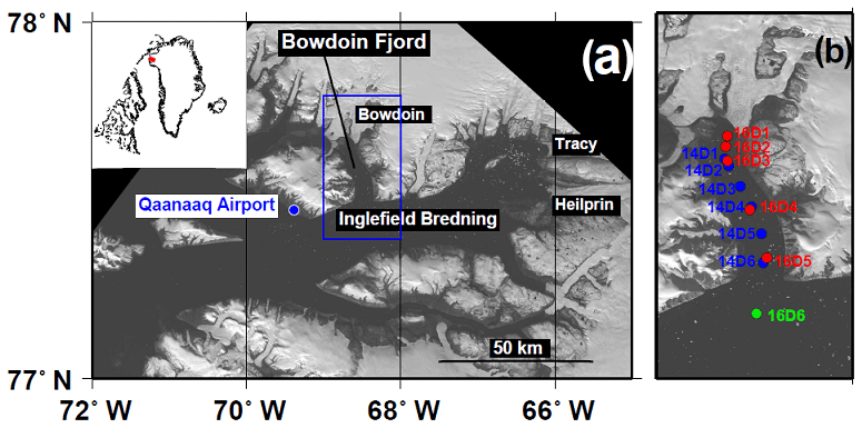
Figure 1Study region in Bowdoin Fjord in northwestern Greenland. (a) Landsat image (6 September 2014) showing northwestern Greenland (downloaded from http://earthexplorer.usgs.gov, last access: 6 April 2020). The blue box indicates the area shown in (b). The inset shows the location of the region in Greenland. (b) Locations of the CTD observation sites indicated by dots (blue in 2014; red in 2016, both inside Bowdoin Fjord; and green in 2016, outside Bowdoin Fjord).
This study focuses on BF (77.6∘ N, 66.8∘ W; 3–5 km wide and 20 km long), one of the arms of Inglefield Bredning (IB; 10–15 km wide and 100 km long) in northwestern Greenland (Fig. 1). In IB, sea ice covers the ocean between October and May. In June and July, the sea ice melts rapidly. During the summer melt season, areas of highly turbid ocean surface water form near the ice sheet and glaciers as a result of glacial meltwater discharge (Ohashi et al., 2016).
The bathymetry of BF was surveyed with an echo sounder along the centerline and several profiles across the fjord (Sugiyama et al., 2015). The water depth is about 600 m at the mouth of BF, shoaling to about 210 m at the ice front of the Bowdoin Glacier (BG). Hence, it is assumed that subglacial discharge takes place at a depth of 210 m below sea level, which corresponds to the depth between warm AW and cold PW cores. Water properties at this depth are expected to change according to the relative influence of AW and PW. Therefore, BF is suitable for assessing the impact of the change in water properties on the vertical distribution of outflowing plume water.
To help estimate the subglacial discharge conditions for BG, we used the Regional Atmospheric Climate Model (RACMO) 2.3p2 runoff data downscaled to 1 km (Noël et al., 2016, 2018). The catchment of the glacier was determined from the Greenland Ice Mapping Project digital elevation model (Howat et al., 2014). In summer (June–August), the daily mean amount of subglacial discharge estimated from the RACMO data varied greatly (19±16 m3 s−1 in 2014 and 21±18 m3 s−1 in 2016). Using the daily mean values of the 5 d prior to the observation dates (Mankoff et al., 2016), we perform numerical experiments (see Sect. 5 for details). The daily mean amount of subglacial discharge over 5 d in 2016 (45 m3 s−1) was estimated to be 25 % greater than that in 2014 (36 m3 s−1).
3.1 Hydrographic observation
We performed CTD observations in BF in the summers of 2014 and 2016. The observations were performed along the centerline of the fjord at six locations each year: at stations 14D1–14D6 on 4 August 2014, and at stations 16D1–16D6 on 29 July 2016 (where the first two digits in the station label denote the year; Fig. 1b). Station 16D6 was located in IB, approximately 4 km from the mouth of BF. A CTD profiler (RINKO Profiler ASTD-102, JFE Advantech) was lowered from a boat to measure the temperature, salinity, and turbidity profiles from the surface to the bottom of the fjord (see Kanna et al., 2018, for details). The precision of the depth, temperature, salinity, and turbidity measurements were 1.8 m, 0.01 ∘C, 0.01 on the practical salinity scale, and 0.3 formazin turbidity units (FTU), respectively.
We collected 33 water samples at stations 16D2–6 to calibrate the salinity measurements. Water sampling was performed at depths deeper than 10 m to avoid the influence of the steep salinity gradient near the surface. The salinities of the water samples were measured using a salinometer (Guideline Autosal 8400B) to correct the in situ measurements based on the CTD. The uncertainty in salinity (∼0.01) made it difficult to compare its absolute value, but the vertical gradient of salinity should be valid.
3.2 Freshwater fraction analysis
In proglacial fjords, seawater is influenced by freshwaters from subglacial meltwater discharge (subglacial discharge) and submarine melting of the ice front (submarine meltwater). A potential-temperature–salinity (θ–S) diagram can be used to separate the mixing processes of these waters (see also Appendix A).
Subglacial discharge mixes with the ambient ocean water to form an upwelling plume, which subsequently spreads due to entrainment. The straight line on the θ–S diagram between the subglacial discharge ( ∘C; pressure dependent freezing point at 210 m depth, ) and ambient ocean water at the conduit depth (θ=θe, S=Se; potential temperature and salinity at the 210 m depth averaged for all observation sites in each year; hereinafter referred to as “entrained fjord water”) is called the runoff line (Straneo et al., 2011, 2012).
At the ice front, submarine melting of ice is driven by the heat of ambient seawater. The straight line on the θ–S diagram that indicates the mixing caused by submarine melting is called the melt line (Straneo et al., 2011, 2012). We defined the effective potential temperature (θmw: ∘C) by calculating the energy required to melt ice when S=0 (Gade, 1979; Jenkins, 1999; Straneo et al., 2012):
where θf is the pressure-corrected melting point of ice (−0.1 ∘C), Lf is the latent heat of fusion (334.5 kJ kg−1), θi is ice temperature (−5 ∘C; Seguinot et al., 2016), and ci and cp are the specific heat capacities of ice and seawater (2.1 and 3.98 ). Thus, the melt line is the line connecting the submarine meltwater (θ=θmw, ) and the entrained fjord water.
In this study, the θ–S data of entrained fjord water were located between the AW and the PW cores, suggesting that the water property was influenced by the mixing of AW and PW. Moreover, the characteristics of AW core differed between 2014 and 2016. Hence, the entrained fjord water property used in this study differed between 2014 and 2016. This entrained fjord water is not necessarily the sole source of submarine meltwater. However, since the observed temperature has a similar structure at the depths where the submarine melt is in effect, we selected the entrained fjord water as the representative source of submarine meltwater fraction (see Sects. 4.2 and 6.3 for details). Note that the estimation of the subglacial discharge fraction is little affected by the above setting of the source due to the θ–S inclination proximity to the melt line.
Assuming that the water properties can be described as a mixture of the three different water masses (subglacial discharge, submarine meltwater, and entrained fjord water), the fraction of each water component in seawater can be calculated (Appendix A; e.g., Everett et al., 2018; Mankoff et al., 2016; Mortensen et al., 2013). In the θ–S space consisting of the positive fraction of each component (hereinafter referred to as the “meltwater quadrant”), the water mass properties can be explained as a mixture of the three components. Note that water mass properties outside the meltwater quadrant are affected by other mixing processes, and the calculation mentioned above is not applicable.
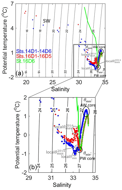
Figure 2(a) Potential-temperature–salinity diagram for the data from 2014 and 2016. Dots are shown at 5 m intervals. The color of the markers corresponds to the sampling sites as indicated in Fig. 1b (blue in 2014, red at stations 16D1–16D5, and green at station 16D6). The potential densities are shown by the black isopycnal contours. The gray box indicates the domain shown in Fig. 7. (b) shows the enlarged region indicated by the gray box in (a).
4.1 Water properties
From the bottom to the surface, layers of warm, saline AW (its core represented by potential temperature maximum; θmax); cold PW (its core represented by the potential temperature minimum; θmin); and specifically warm, fresh SW were observed in 2014 and 2016 (Fig. 2). In 2016, the θ–S properties were similar at depths deeper than the PW core inside and outside BF. However, at depths shallower than the PW core, the θ–S properties differed. Outside BF, temperature monotonically increased from the PW core toward the surface, suggesting the development of a seasonal pycnocline. Inside BF, temperature increased upwards but then decreased at about 40 m. This difference was suggestive of local characteristics of the fjord water structure. Between 2014 and 2016, there were several differences in water properties, especially in temperature. The vertical distributions of the potential temperature, salinity, and turbidity as well as their differences are described in the subsequent sections.
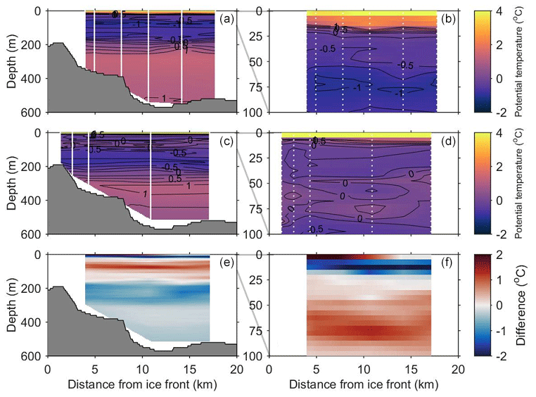
Figure 3Contour plots of potential temperature along the centerline of Bowdoin Fjord as observed in (a) 2014 and (c) 2016. The difference between the 2 years (2016–2014) is shown in (e). (b), (d), and (f) show the enlarged region from the sea surface to 100 m.
4.1.1 Potential temperature
The AW core was warmer and shallower in 2014 (1.3 ∘C at ∼290 m) than in 2016 (1.0 ∘C at ∼320 m; Fig. 3a–d). At the deepest part of the fjord, the warm layer (>0 ∘C) was thicker in 2014. Moreover, the depth of the PW core was shallower in 2014 with a temperature of −0.8 ∘C in both 2014 and 2016. Because of the differences in the AW core temperature and warm layer thickness, the temperature near the BG drainage conduit (210 m) was up to 0.9 ∘C warmer in 2014 (Fig. 3e).
At depths shallower than 150–170 m (i.e., PW core), the temperature structure differed significantly between the two observations. In 2014, a relatively cold temperature maximum (−0.7 ∘C; hereinafter referred to as “local ”) was found at a depth of 100 m (Figs. 2, 3a, b). Moreover, the coldest water (−1.0 ∘C; hereinafter referred to as “local θmin”) was observed at a depth of 80 m (Figs. 2, 3a, b), and the temperature at the local θmin was even colder than that at the PW core. In 2016, a corresponding local θmin was not observed, but a clear temperature maximum (0.2 ∘C; hereinafter referred to as “local ”) was found at a depth of 60 m and the temperature of the local was significantly warmer than that of the local (Figs. 2, 3c, d). Because the increase in temperature from the PW core to the local in BF was roughly the same as that outside BF, the water properties below the local layer in the fjord could represent a seasonal pycnocline over a wider area. In addition, the difference between local and local suggested that a more enhanced seasonal pycnocline developed in 2016 compared to 2014.
At depths shallower than 20 m, the water temperature increased rapidly toward the surface in both 2014 and 2016. However, the temperatures were up to 2.3 ∘C colder in 2016 than in 2014 at depths of 5–20 m (Fig. 3e and f).
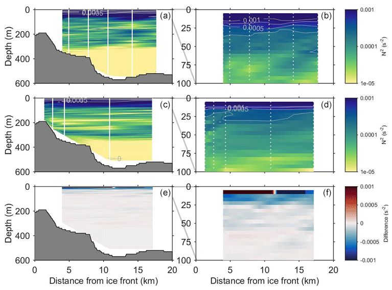
4.1.2 Salinity, potential density, and stratification
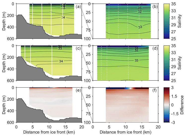
At depths below 210 m, including the AW core, salinity was roughly the same between the two observations (Fig. 4a–d), although the salinity at the AW core differed (2014: 34.2, 2016: 34.3). At a depth of 5–170 m (shallower than the PW core), salinity was higher in 2016 than in 2014, including the salinity at the PW core (2014: 33.5, 2016: 33.7) (Fig. 4e and f). This difference was more significant (0.6–1.6) near the surface (5–20 m). In contrast, salinity at the surface (0–5 m) was lower in 2016 except at the outer portion of BF.
The vertical distribution of the potential density was mainly controlled by salinity; therefore, the differences in the potential density between 2014 and 2016 were mostly the same as those of salinity (not shown). At a depth of 5–170 m, the potential density was higher in 2016 than in 2014, while at the surface it was lower in 2016.
Behavior of subglacial discharge plume is affected by salinity and density profiles. The square of the Brunt–Väisälä frequency (N2) increased toward the surface in both observations. In particular, N2 was the greatest (>0.001 s−2) at depths shallower than 10–15 m, representing the strongest stratification among all depths (Fig. 5a–d). N2 was higher in 2016 than in 2014 at depths shallower than 10 m but lower by up to 0.0007 s−2 at depths of 10–50 m (Fig. 5e and f). Thus, the stratification in 2016 was stronger near the surface (0–10 m) than in 2014 but weaker at the subsurface (10–50 m).
4.1.3 Turbidity
Turbidity acts as an effective tracer of subglacial discharge plume. The highest turbidity layer (>4 FTU) was found not at the surface but at the subsurface at 15–50 m in 2014 and 10–40 m in 2016 (Fig. 6a–d). Turbidity decreased from the subsurface to a depth of about 100 m, and it reached almost zero at depths below 150 m. In addition, turbidity decreased with distance from the ice front toward the mouth of the fjord, in contrast to temperature and salinity, which changed little horizontally.
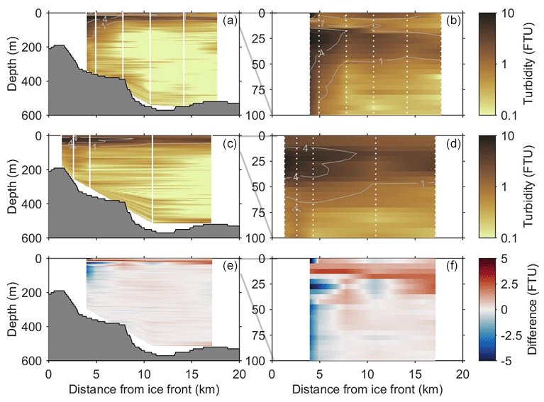
The distribution in turbidity differed between the two observations. In 2014, a low-turbidity layer existed further offshore at a depth of around 10 m, which was sandwiched by higher turbidities above and below (Fig. 6a and b). Conversely, in 2016, turbidity was nearly homogeneous at the depth range of 0–15 m, and there was no discontinuity at a depth of 10 m (Fig. 6c and d). Therefore, turbidity at a depth of 0–15 m was 1–2 FTU higher in 2016 than in 2014 (Fig. 6e and f). Meanwhile, at the depth of 40–150 m within 5 km of the ice front in 2014, turbidity was relatively high (>1 FTU). In 2016, no relatively high-turbidity layer existed at depths below around 60 m. Therefore, turbidity at a depth of 15–200 m within 5 km of the ice front was lower in 2016 than in 2014. This difference was particularly significant (up to 1.5–5 FTU) at depths of 20–120 m. These differences in turbidity could be attributed to the fraction of subglacial discharge, as will be discussed in Sect. 4.2.
4.2 Freshwater fraction in θ–S diagram and the role of subglacial discharge
As shown in Sect. 4.1, there were some differences in the vertical distribution of the θ–S properties between 2014 and 2016. To understand the differences in the mixing processes controlling the water properties, we estimated the freshwater fractions in the θ–S diagram (see Sect. 3.2 for details). We compared a common site nearest the ice front (stations 14D1 and 16D3; approximately 4 km from the ice front) and examined the difference in the freshwater fractions. The results were similar for the other stations regardless of distance from the ice front (e.g., stations 14D4 and 16D4 with ∼11 km distance from the ice front).
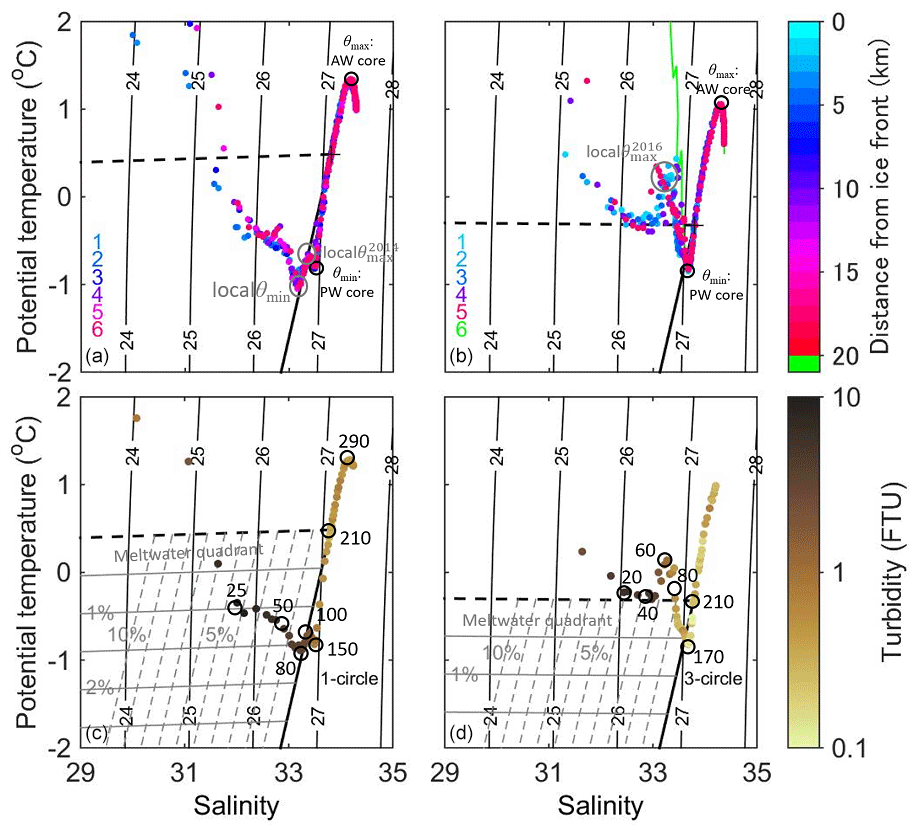
Figure 7Potential-temperature–salinity diagrams of the freshwater fractions in (a), (c) 2014 and (b), (d) 2016 (as shown in Fig. 2b). The solid and dashed black lines represent the theoretical melt and runoff line, respectively. In (a) and (b), the data are plotted for stations 1–6, and the color scale indicates the station number. In (c) and (d), the data are plotted for stations with ∼4 km distance from the ice front (14D1 and 16D3 at depths ≥5 m). The color of markers denotes turbidity. The solid and dashed gray lines represent the fractions of submarine meltwater (where the line intervals are 0.5 %–2.5 %) and subglacial discharge (where the line intervals are 1 %–10 %), respectively. The black numbers outside the circles indicate the depth.
First, we examined the properties of the entrained fjord water at the 210 m depth. The θ–S properties obtained in 2014 were closer to those of the AW core than the PW core (Fig. 7a and c), whereas those in 2016 were closer to the PW core (Fig. 7b and d). This difference implies greater influence of AW at the 210 m depth in 2014.
At depths from 210 m to the PW core (∼150 m), the θ–S properties in 2014 showed a similar tendency as those in 2016. In both 2014 and 2016, near the PW core, the θ–S properties deviated slightly from the melt line and were located outside the meltwater quadrant.
The θ–S properties above the PW core (80–150 m) differed between 2014 and 2016. The θ–S properties in 2014 deviated slightly toward a high temperature from the PW core to the local (∼100 m). This deviation might reflect a slightly developed seasonal pycnocline. From the local (∼100 m) to the local θmin (∼80 m), the θ–S properties aligned perfectly along the melt line (solid black lines in Fig. 7a and c). The submarine meltwater fraction at the local θmin was estimated to be 1.6 %, which was the largest fraction, indicating the greatest influence of submarine melting among all depths (Fig. 7c). The estimated submarine meltwater fraction at the local θmin increased to 2.1 % and 2.5 % in the case that the source of entrained fjord water was set to the water at the depth of 250 and 300 m, respectively. Meanwhile, the subglacial discharge fraction was not significant. By contrast, in 2016, the θ–S properties were indicative of a seasonal pycnocline above the PW core, and the submarine meltwater fraction decreased to less than 0.5 % (Fig. 7d). The estimated fraction increased to 1.1 % and 1.8 % in the case that the source of entrained fjord water was set to the water at the depth of 250 and 300 m, respectively, but the submarine meltwater fraction was by far smaller than those in 2014. On the other hand, the subglacial discharge fraction was estimated to be 1.1 %.
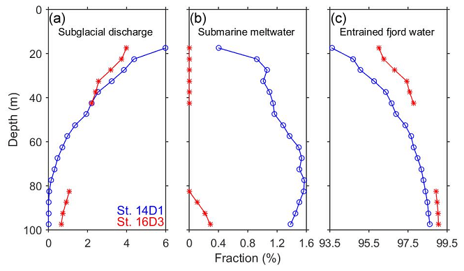
Figure 8Vertical profiles of the three water mass fractions of (a) subglacial discharge, (b) submarine meltwater, and (c) entrained fjord water at stations 14D1 (blue) and 16D3 (red).
At depths of 50–80 m, above the local θmin in 2014, the seawater consisted of 1.3 %–1.6 % submarine meltwater, 0.1 %–1.4 % subglacial discharge, and 97.3 %–98.3 % entrained fjord water (Fig. 7c and blue lines in Fig. 8). This mixture reflected the substantial influence of submarine meltwater in this layer. In 2016, the θ–S data were located outside the meltwater quadrant, implying that the ocean water properties could not be explained by the simple mixing of the three water components (Fig. 7b and d). Near the local approximately 60 m, turbidity was significantly lower in 2016 than in 2014, implying a weaker influence of subglacial discharge.
Further upward, we focused on the subsurface at a depth of 15–40 m where the highest turbidity was observed. The subglacial discharge fraction was high, with a maximum around 15 m (Fig. 7c and d). In 2014, the seawater consisted of 2.5 %–6.0 % subglacial discharge, 0.4 %–1.1 % submarine meltwater, and 93.6 %–96.3 % entrained fjord water (Fig. 7c and blue lines in Fig. 8). Although the submarine meltwater fraction decreased closer to 15 m, the rapid increase in temperature in the θ–S diagram might reflect the influence of the development of a seasonal pycnocline. In 2016, the seawater was composed of approximately 2.4 %–4.0 % subglacial discharge and 96.0 %–97.6 % entrained fjord water, with no submarine meltwater (Fig. 7d and red lines in Fig. 8). The subglacial discharge fraction was up to 2.0 % greater in 2014 than in 2016.
Near the surface (depth: 5–15 m) immediately above the most turbid water layer, the θ–S properties were outside the meltwater quadrant in both observations. The θ–S properties in 2014 deviated toward a significantly high temperature and low salinity above the runoff line (Fig. 7a and c). The θ–S properties in 2016 showed a similar tendency to 2014, but the deviation from the runoff line was smaller (Fig. 7b and d). Therefore, water might have been influenced by subglacial discharge more strongly in 2016 than in 2014, although it was difficult to quantify, because this layer was outside the meltwater quadrant. Turbidity at this depth was also higher in 2016 than in 2014, supporting the greater influence of subglacial discharge in 2016.
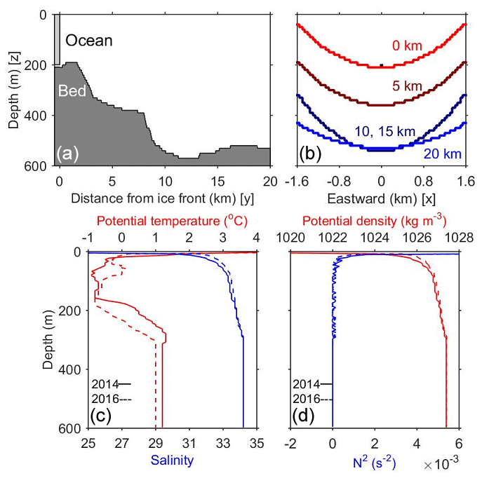
Figure 9Numerical model settings. (a) Ocean depth along the centerline of Bowdoin Fjord (from north to south). The space between the glacier and the sea bed indicates a 10 m high subglacial drainage conduit. (b) Depth across the fjord (from west to east) at 0, 5, 10, 15, and 20 km from the ice front. The box indicates the subglacial drainage conduit at the center of the fjord (40 m wide × 10 m high; 400 m2). Initial vertical profiles of (c) potential temperature, salinity, (d) potential density, and the square of Brunt–Väisälä frequency (N2) computed from (c).
5.1 Experimental settings
To interpret the observed differences in the vertical distribution of outflowing plume water between 2014 and 2016, we perform a set of numerical model experiments. The model simulates a transient behavior of the subglacial discharge plume in front of the BG (Fig. 9). We use a three-dimensional nonhydrostatic ocean model with the Boussinesq approximation, originally developed by Matsumura and Hasumi (2008). The model domain represents BF and is 3.2 km wide (from east to west; x direction), 20.5 km long (from north to south; y direction), and 600 m deep (z direction) (Fig. 9a and b). The ice front is located at the northern end and the fjord mouth at the southern end. We simplify the measured bathymetry of the BF (Sugiyama et al., 2015; Fig. 9a and b) to set a model geometry. A subglacial drainage conduit is approximated by a rectangular channel (40 m wide × 10 m high) at the base (210 m deep) in the center of the glacier front. The model resolution is 20 m horizontally and 5 m vertically. The horizontal subgrid-scale viscosity and diffusion are represented by the strain rate-dependent Smagorinsky model (Smagorinsky, 1963) following Matsumura and Hasumi (2010). The vertical viscosity and diffusivity coefficients are set to m2 s−1. The Coriolis parameter is set to s−1.
The initial potential temperature and salinity are set to be horizontally uniform using the observation data in 2014 (solid lines in Fig. 9c and d). Subglacial discharge ( ∘C; pressure dependent freezing point at 210 m depth, S=0) is injected into the model domain from the subglacial drainage conduit at the northern boundary. The velocity profile at the southern boundary is predicted to compensate for the discharge inflow so that the total water volume is conserved in the model domain. A virtual tracer, that is assumed to obey the same advection–diffusion equation as potential temperature and salinity, is implemented to track the behavior of subglacial discharge. The tracer concentration is initially zero over the whole domain and exhibits unity for the subglacial discharge. No heat flux and wind stress are applied at the surface. Quadratic drag bottom condition is used for the seafloor, where the non-dimensional drag coefficient is set to . We restore θ and S to the initial profile at the southern boundary. The model is integrated for 7 d from a state of rest, which is sufficient time for the subglacial discharge tracer to reach the southern boundary. Note that the numerical experiment results represent the transitional process of the subglacial discharge tracer, and they are not applicable to a long-term behavior of subglacial plume. Thus, we do not discuss the response of the fjord stratification to the water mass transformation due to plume entrainment on the timescales of months.
Table 1List of model runs. Run names, initial stratifications, and values of inflow velocity (Vsg: m s−1) and flux of subglacial discharge (Qsg: m3 s−1).
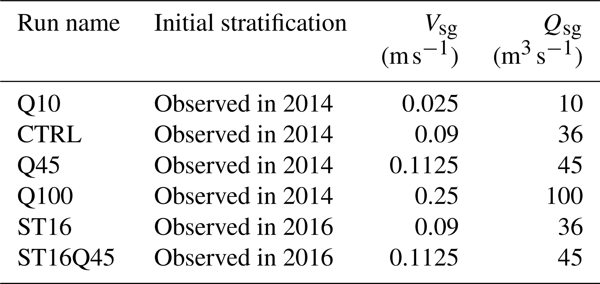
As the control case, we perform the experiment given by inflow velocity at the northern boundary (Vsg) of 0.09 m s−1, corresponding to the subglacial discharge (Qsg) of 36 m3 s−1 (estimated from the RACMO data in Sect. 2) (hereinafter referred to as CTRL; Table 1). To investigate the effect of the amount of subglacial discharge, the experiments are conducted by changing the inflow velocity by a factor of 10 (Vsg=0.025, 0.1125, and 0.25 m s−1; Qsg=10, 45, and 100 m3 s−1; hereinafter referred to as Q10, Q45, and Q100, respectively). We also perform the experiments with the same subglacial discharge as the CTRL and Q45 but with the initial stratification as observed in 2016 to assess the influence of the stratification difference (hereinafter referred to as ST16 and ST16Q45, respectively; dashed lines in Fig. 9c and d).
Although we have implemented the effect of submarine melting following Holland and Jenkins (1999) and Losch (2008), the amount of resultant meltwater is less than 0.05 % of the imposed subglacial discharge. Hence, the effect of submarine melting is negligible on the timescale considered with the present model settings.
5.2 Experimental results
Numerical experiments are performed to investigate the impact of the 25 % greater discharge (Q45), fjord stratification (ST16), and their combined impact (ST16Q45) as compared to the most realistic case (CTRL; see Appendix B for details). When comparing the results of CTRL with those of Q45, ST16, and ST16Q45, the results after 41 h are used to consider the integration time required for the virtual tracer to reach the southern boundary in the earliest case. A comparison of the CTRL and ST16Q45 results is shown in Appendix C.

Figure 10(a) Cross-fjord averaged difference between subglacial discharge tracer concentrations for Q45 (Qsg=45 m3 s−1) and CTRL (Qsg=36 m3 s−1) using the same initial stratification conditions. The difference after integration for 41 h is shown. (b) Difference between the results for the same amount of discharge using initial stratifications as observed in 2016 and 2014 (ST16–CTRL). (c) and (d) Percentage of the results in (a) and (b), respectively.
In Q45, the subglacial discharge tracer concentration at a depth of 0–50 m is 10 %–60 % greater than that in CTRL (Fig. 10a and c). In addition, the tracer concentration shows a decrease of 10 %–40 % at deeper depths of 50–80 m only in the vicinity of the glacier front. This indicates that subglacial discharge plume shifts to the shallower layer as the amount of discharge increases.
In ST16, the concentration of subglacial discharge tracer at a depth of 0–25 m is up to 60 % greater than that in CTRL, except at a depth of 5–15 m in the vicinity of the glacier front (Fig. 10b and d). In particular, at a depth of 0–5 m, tracer concentration rate of increase is high. At depths below 25 m, the tracer concentration decreases by up to 50 %. The stratification in ST16 in the subsurface layer is weaker than that in CTRL. Weaker stratification favors stronger upwelling. The plume in ST16 is likely to spread near the surface in higher concentrations than that in CTRL.
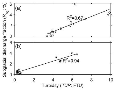
Figure 11Scatter plots of turbidity and the subglacial discharge fraction at stations (a) 14D1 (data in the meltwater quadrant of Fig. 7c) and (b) 16D3 (data in the meltwater quadrant and that including the data points at a depth of 15–40 m in Fig. 7d). The solid lines represent the linear regression of the data.
6.1 Quantitative relationship between the subglacial discharge fraction and turbidity
In Sect. 4.2, it was shown that high turbidity corresponded to a high fraction of subglacial discharge. Therefore, we assessed the quantitative relationship between turbidity and subglacial discharge fraction in both study years (Fig. 11). In 2014, the relationship between the subglacial discharge fraction (Rsg:%) and turbidity (TUR:FTU) in the meltwater quadrant was expressed as –2.0 (R2=0.67; Fig. 11a). In 2016, the data in the meltwater quadrant and that including the data points close to the runoff line (depth: 15–40 m) showed a linear relationship of (R2=0.94), with a roughly similar inclination to that in 2014 (Fig. 11b). Moreover, the low turbidity at the local (depth: 60 m) in 2016 was consistent with the calculation that the fraction of subglacial discharge is small in this layer (Fig. 7b and d). These results indicate that the vertical distribution of turbidity reflects the mixing ratio of subglacial discharge near the ice front (Fig. 6).
Recent observations in other regions of Greenland have qualitatively shown that the high-turbidity subsurface layer corresponds to the vertical distribution of outflowing plume water (Chauché et al., 2014; Stevens et al., 2016). The quantitative relationship between turbidity and the subglacial discharge fraction presented in this study reveals that measuring turbidity is an effective tool to investigate the vertical distribution of outflowing plume water into fjords. At the fjord surface, the quantitative relationship between turbidity and the subglacial discharge fraction was not investigated in this study. It should be noted that turbidity at the fjord surface is only a reasonable proxy if turbid subglacial discharge plume is able to reach the surface, which depends on the degree of entrainment.
6.2 Factors controlling the observed vertical distribution of outflowing plume water
As shown in Sect. 4.2, the estimated subglacial discharge fraction differed between 2014 and 2016. A likely interpretation of this difference is the amount of subglacial discharge and fjord stratification in each observation. To test this hypothesis, we compare the numerical model results with the observational data. It should be noted that the observational data represent snapshots in summer and not the entire melt seasons. Thus, we discuss only the difference in the short-term transitional process of outflowing plume water.
Near the fjord surface (depth: 5–15 m), turbidity was higher in 2016 than in 2014 (Fig. 6e and f). In Q45, the concentration of subglacial discharge tracer near the surface increased by about 30 % from that in CTRL (Fig. 10a and c). The observation and model were consistent with the assumption that the subglacial discharge in 2016 was greater, as estimated from the RACMO data. These results suggest that turbid subglacial plume extended near the fjord surface more in 2016 because of a stronger buoyancy forcing exerted by the 25 % greater discharge. Previous studies have also suggested that a subglacial plume driven by a greater discharge has a stronger buoyancy forcing, leading to both faster entrainment of ambient water and an increase in the fraction of subglacial discharge (Jenkins, 2011; Straneo and Cenedese, 2015). Chauché et al. (2014) compared the θ–S properties of fjord water with the amount of subglacial discharge based on a glacier surface melt estimation using a positive-degree-day/melt-rate model (Box, 2013). Comparison of results in CTRL and Q45 showed that a 25 % change in the subglacial discharge caused an approximately 30 % change in the subglacial discharge fraction near the surface. In ST16, the tracer concentration increased by a large portion in 5–15 m compared to that in CTRL (Fig. 10b and d). Although the increase at 5–15 m favored the observed change, the mean increase in the tracer concentration was smaller than that of the increase in discharge. Therefore, the vertical distribution of outflowing plume water near the surface could be affected more by a change in the amount of subglacial discharge than the difference in the observed fjord surface stratification.
Furthermore, a 25 % increase in the subglacial discharge results in a greater tracer concentration not only at the surface but also at the subsurface (depth: 15–40 m). The magnitude of the change was similar between the surface and subsurface layers (a few tens of percent) (Fig. 10a and c). This implies the need to consider the vertical distribution of outflowing plume water at the subsurface in addition to the drone surface measurement to quantitatively assess the overall impact of subglacial discharge.
In contrast to the observations near the surface, the fraction of turbid subglacial discharge at the subsurface (15–40 m) was greater in 2014 than in 2016 (Figs. 6, 7, and 8a). This field observation was inconsistent with the numerical experiments of the differences in discharge, showing a smaller concentration of subglacial discharge tracer at the subsurface under a smaller amount of discharge (Fig. 10a and c). From the stratification change experiment, the tracer concentration at 25–40 m was about 20 % greater in CTRL than in ST16 (Fig. 10b and d). Although the decrease in the shallow portion of subsurface did not favor the observed change, this was consistent with the observed difference at the subsurface, and the rate of change was quantitatively consistent (a few tens of percent). Thus, in comparison of the change in the amount of subglacial discharge, variations in stratification are a likely explanation for the observed differences in the subglacial discharge fraction at the subsurface.
Previous studies have shown that strong subsurface stratification in fjords prohibits upwelling of the subglacial discharge plume and results in the dispersion of the plume into a subsurface layer (Carroll et al., 2015). Furthermore, plumes extend further over the surface under weaker stratification (Carroll et al., 2015). The stratification in ST16 in the subsurface layer is weaker than that in CTRL, whereas that near the surface is stronger. In the case when the plume reached the fjord surface, our model suggested that strong surface stratification would prohibit the subduction of the outcropped plume, likely resulting in a plume that extends to the fjord surface.
6.3 Difference in the formation process of stratified structures
Subsurface stratification influences the vertical distribution of outflowing plume water. The fjord stratification in 2014 and in 2016 differed at a depth of approximately 60–80 m, which was attributed to the influence of submarine melting and the broad seasonal pycnocline. In this section, we discuss the formation process of the stratified structures in each observation.
In 2014, a warm layer strongly affected by AW was in contact with the ice front, which could enhance the fraction of submarine meltwater around a depth of 80 m (Figs. 2, 3, 7a, c, and 8b). Because the submarine meltwater fraction was detected regardless of the distance from the ice front of the BG, submarine meltwater from other glaciers in IB might have influenced the water in BF. Moreover, this horizontal distribution of the submarine meltwater suggests that the submarine melt does not take place only at the subglacial conduit depth. However, the relationship that temperature at the deep part of fjord is generally warmer in 2014 and the relatively warmer source temperature of entrained fjord water in 2014 should be robust (Figs. 3 and 7). A warm layer above 210 m extended further up to the shallower layer in 2014 than in 2016. The available excess heat was 1.6 times greater in 2014 than in 2016 when calculated by the difference from the freezing temperature (Figs. 3 and 7). A previous model study found that the rate of submarine melting increased proportionally to the increase in water temperature to the power of 1.3–1.6 (Xu et al., 2013). Porter et al. (2014) revealed that the rates of ice mass loss at the Tracy Glacier and Heilprin Glacier, neighboring tidewater glaciers in IB, differed substantially between 1.63 and 0.53 Gt a−1. Since the water depth at the ice front of the Tracy Glacier (610 m) is deeper than that of the Heilprin Glacier (350 m), the ice front has wider contact with warm AW, suggesting a greater glacier mass loss associated with the greater submarine melting (Porter et al., 2014). Our study suggests that the difference in the structure of deep heat storage can alter the development of submarine melting layer and affects ice mass loss from Greenland glaciers.
In 2016, a simple, but broad, seasonal pycnocline was detected outside BF (Figs. 2, 3, 7b, and d). In the study area (Qaanaaq Airport; 77.47∘ N, 69.23∘ W; 16 m a.s.l.; blue circle in Fig. 1a), the mean temperature during the previous winter (December–February) was 1.1 ∘C lower in 2016 than in 2014. Thus, winter vertical mixing of the fjord was enhanced and the mixed layer depth could deepen during the preceding winter in 2016. In summer, a seasonal pycnocline could develop above the remnant of the winter mixed layer. In addition, the PW core in BF was deeper in 2016, supporting the possibility of the development of a seasonal pycnocline influenced by the enhancement of the winter vertical mixing. We speculate that the development of the seasonal pycnocline over a broader area in 2016 is due to the enhancement of winter vertical mixing.
At depths shallower than 60–80 m, where subglacial discharge spreads, fjord stratification could be modified by subglacial discharge. Fjord stratification is expected to be stronger after subglacial discharge that exits near the surface as in this study, because subglacial discharge would lighten the surface layers. However, this study revealed the transitional processes of subglacial discharge plume over a relatively short timescale. To fully understand the longer-term interactions of subglacial discharge and fjord stratification (e.g., seasonal and interannual variations), we need to perform long-term oceanic observations and numerical experiments to capture the realistic nature of discharge and submarine melting over a much broader model domain.
With a focus on the differences in the vertical distribution of outflowing plume water and ambient water properties, we investigated the properties of vertical water mass profiles in BF in northwestern Greenland. The differences in the subglacial discharge fraction and water mass properties between 2014 and 2016 are summarized in Fig. 12.
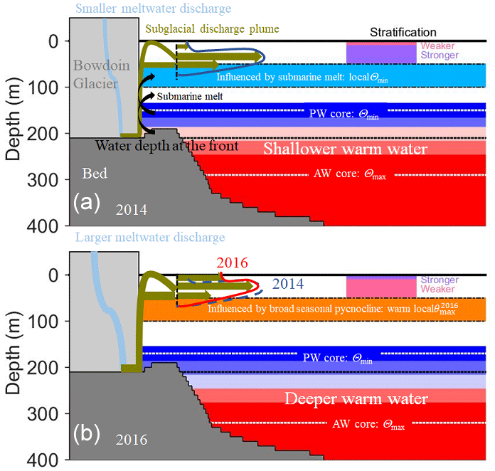
Figure 12Schematic diagram of the possible glacial discharge and properties of vertical water mass profiles of Bowdoin Fjord in (a) 2014 and (b) 2016.
The depths of the temperature minimum and maximum differed between the two observations. The θmax (AW core) and the θmin (PW core) were shallower in 2014 (θmax at ∼290 m; θmin at ∼150 m) than in 2016 (θmax at ∼320 m; θmin at ∼170 m). The local θmin was observed around 80 m in 2014 but not in 2016. In turn, prominent local was detected around 60 m in 2016, which was significantly warmer than the local maximum in 2014. The analysis of the θ–S properties indicated that local θmin in 2014 and local in 2016 could be influenced by the development of a submarine melting layer and broad seasonal pycnocline, respectively.
Subglacial discharge plume spread at a depth shallower than local θmin and local . In both 2014 and 2016, the fractions of turbid subglacial discharge were highest at the subsurface (15–40 m). The maximum fraction near the ice front was ∼6 % in 2014 and ∼4 % in 2016. Near the surface (5–15 m), turbidity was higher in 2016 than in 2014, suggesting a stronger influence of turbid subglacial discharge in 2016.
To assess the factors controlling the difference in the observed subglacial discharge fraction, we perform a set of numerical experiments to simulate the subglacial discharge plume under different stratification and volume flux of subglacial discharge. The experiments using the different initial stratifications suggest that the fractional difference in subglacial discharge at the subsurface is likely attributed to the difference in fjord stratification. Moreover, the numerical model results based on a 25 % greater discharge suggest that the difference near the surface is primarily affected by the increase in discharge.
From the surface to the subsurface, where subglacial discharge spreads, fjord stratification varied between the study years depending on the layer that developed and the amount of subglacial discharge. At a depth around 60–80 m, fjord stratification could be determined by the influences of submarine melting and seasonal pycnocline. Because of the thicker warm layer strongly affected by AW, a submarine melting layer was able to develop in 2014.
Our study suggests that observed fjord stratification, together with the amount of subglacial discharge, can affect the vertical distribution of outflowing plume water. Given the current increase in meltwater discharge from Greenlandic glaciers, the buoyancy forcing of the subglacial discharge plume and ambient fjord stratification are expected to change. To fully capture the behavior of subglacial discharge plume, further continuous observations and numerical modeling are required over a wider area encompassing northwestern Greenland.
The origins of freshwater in ocean water can be estimated based on a three-water mass mixing model. To quantitatively assess the difference in freshwater fractions, we calculated the volume fractions of subglacial discharge (fsg), submarine meltwater (fmw), and entrained fjord water (fe) from the observed temperature and salinity (Fig. A1). From the mass conservation of fsg, fmw, and fe:
The sampled potential temperature (θA: ∘C) and salinity (SA) are represented in the following equations:
Because Ssg=0 and Smw=0, Eq. (A3) is converted into
Using Eqs. (A1), (A2), and (A4), fsg and fmw are given as the following respective equations:
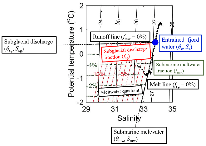
Figure A1Freshwater fraction analysis in the potential-temperature–salinity diagram. The black dots represent the data observed at depths ≥5 m of station 14D1.
To validate the transitional process of subglacial discharge obtained from the numerical experiment, we compare the numerical model results (CTRL, Q100, and Q10) with observation condition.
In CTRL, the highest tracer concentration is observed at a depth of 0–5 m within several hundreds of meters from the ice front and at a depth of 10–15 m beyond several hundreds of meters from the ice front (Fig. B1a). The distribution roughly coincides with the observed profiles.
In Q100, beyond several hundreds of meters from the ice front, the highest tracer concentration is observed at a depth of 10–15 m, approximately the same results as obtained in CTRL (Fig. B1b). However, the region of the highest tracer concentration covers up to 1.0×10⁵ m2 of the fjord surface (Fig. B1e and h), which is not detected at the BG ice front during the 2 years of observations.
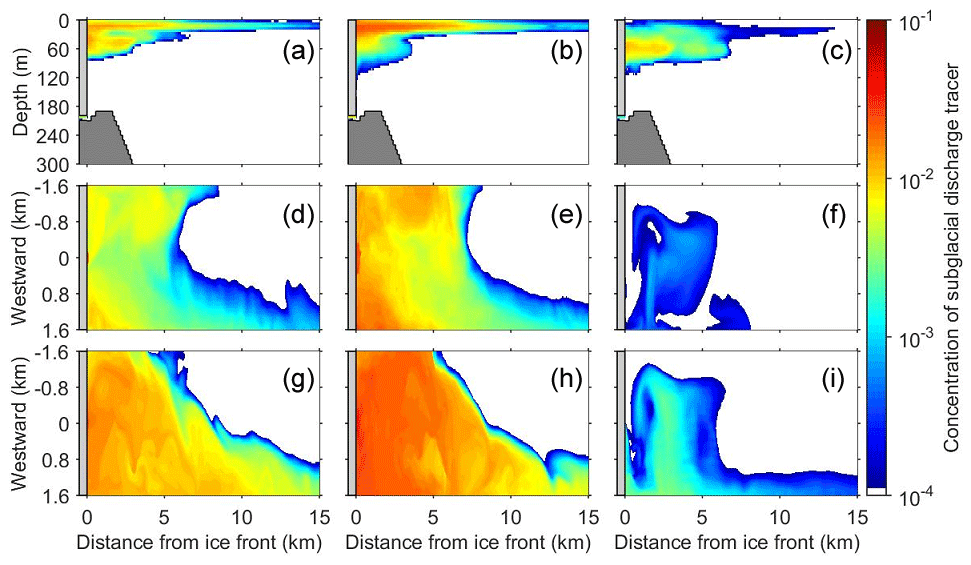
Figure B1(a–c) Cross-fjord averaged concentration of the subglacial discharge tracer. Horizontal distribution of the tracer concentration (d–f) at the fjord surface (depth: 0–5 m) and (g–i) at a depth of 10–15 m. Experimental results are obtained (a, d, g) in CTRL after integration for 62 h (b, e, h) in Q100 after 33 h, and (c, f, i) in Q10 after 153 h. The integration time in each experiment is equivalent to the time required for the first arrival of the tracer.
In Q10, the highest concentration of subglacial discharge tracer is observed at a depth of 50–60 m regardless of the distance from the ice front (Fig. B1c). This result is significantly different from those in CTRL and Q100. The results indicate that subglacial discharge plume does not reach the fjord surface, which is inconsistent with the visual observation of turbid surface plumes in front of BG.
In summary, among the three experiments performed under the same initial stratification, the results of CTRL, using the subglacial discharge estimated from RACMO data, are the most consistent with the observed horizontal and vertical distributions of plume water.
To investigate the combined impact of the 25 % greater discharge and fjord stratification difference (ST16Q45), a numerical experiment is performed. In ST16Q45, the concentration of subglacial discharge tracer at a depth of 0–30 m is 30 %–60 % greater than that in CTRL, whereas the tracer concentration decreases by up to 60 % at depths below 30 m (Fig. C1a and b). The results are consistent with the observed differences at 5–15 m (near the surface) and 30–40 m (deep portion of the subsurface), except at the depth of 15–30 m. This supports the suggestion that the vertical distribution of outflowing plume water near the surface and at the subsurface can be affected by the differences in the amount of discharge and fjord stratification, respectively (Sect. 6.2).
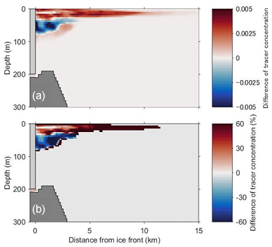
Figure C1(a) Cross-fjord averaged difference between the results for the different amounts of discharge, using initial stratifications as observed in 2016 and 2014 (ST16Q45–CTRL). The difference after integration for 41 h is shown. (b) Percentage of the results in (a).
The codes to generate the figures and analysis are available from Zenodo (https://zenodo.org/record/3532803, last access: 6 April 2020; Ohashi et al., 2019). The source code for the nonhydrostatic ocean model used in this study is available at http://lmr.aori.u-tokyo.ac.jp/feog/ymatsu/kinaco.git (last access: 6 April 2020).
Air temperature data are provided by the United States National Oceanic and Atmospheric Administration National Climatic Data Center (http://www.ncdc.noaa.gov/cdo-web/, last access: 6 April 2020). The CTD data and all files used in the numerical experiments are available from Zenodo (https://zenodo.org/record/3532803, last access: 6 April 2020; Ohashi et al., 2019).
YO analyzed data, performed simulations, and produced figures. YO and SA prepared the article. YM developed the model code. SS, NK, DS, and YO contributed to the field work. All authors discussed the results and commented on the article.
The authors declare that they have no conflict of interest.
We would like to thank Yasushi Fukamachi, Takanobu Sawagaki, Jun Saito, Izumi Asaji, and the members of the 2014 and 2016 field campaigns. Special thanks are extended to Sakiko Daorana, Toku Oshima, and Kim Petersen for providing logistical support. We would like to acknowledge Michiel Roland van den Broeke and Brice Noël for providing RACMO data.
This research has been supported by the Japanese Ministry of Education, Culture, Sports, Science and Technology through the Green Network of Excellence (GRENE) Arctic Climate Change Research Project and the Arctic Challenge for Sustainability (ArCS) Project, and JSPS KAKENHI (grant nos. JP16K12575, JP15H05825, JP16H05734, and JP20H00186).
This paper was edited by Mario Hoppema and reviewed by two anonymous referees.
Arendt, K. E., Dutz, J., Jónasdóttir, S. H., Jung-Mads, S., Mortensen, J., Møller, E. F., and Nielsen, T. G.: Effects of suspended sediments on copepods feeding in a glacial influenced sub-Arctic fjord, J. Plankt. Res., 33, 1526–1537, https://doi.org/10.1093/plankt/fbr054, 2011.
Bartholomaus, T. C., Amundson, J. M., Walter, J. I., O'Neel, S., West, M. E., and Larsen, C. F.: Subglacial discharge at tidewater glaciers revealed by seismic tremor, Geophys. Res. Lett., 42, 6391–6398, https://doi.org/10.1002/2015GL064590, 2015.
Bendtsen, J., Mortensen, J., Lennert, K., and Rysgaard, S.: Heat sources for glacial ice melt in a West Greenland tidewater outlet glacier fjord: The role of subglacial freshwater discharge, Geophys. Res. Lett., 42, 4089–4095, https://doi.org/10.1002/2015GL063846, 2015.
Box, J. E.: Greenland Ice Sheet Mass Balance Reconstruction. Part II: Surface Mass Balance (1840–2010), J. Climate, 26, 6974–6989, https://doi.org/10.1175/JCLI-D-12-00518.1, 2013.
Cape, R. M., Straneo F., Beaird N., Bundy, R. M., and Charette, M. A.: Nutrient release to oceans from buoyancy-driven upwelling at Greenland tidewater glaciers, Nat. Geosci., 12, 34–39, https://doi.org/10.1038/s41561-018-0268-4, 2019.
Carroll, D., Sutherland, D. A., Shroyer, E. L., Nash, J. D., Catania, G. A., and Stearns, L. A.: Modeling turbulent subglacial meltwater plumes: Implications for fjord-scale buoyancy-driven circulation, J. Phys. Oceanogr., 45, 2169–2185, https://doi.org/10.1175/JPO-D-15-0033.1, 2015.
Carroll, D., Sutherland, D. A., Shroyer, E. L., Nash, J. D., Catania, G. A., and Stearns, L. A.: Subglacial discharge-driven renewal of tidewater glacier fjords, J. Geophys. Res.-Oceans, 122, 6611–6629, https://doi.org/10.1002/2017JC012962, 2017.
Catania, G. A., Stearns, L. A., Sutherland, D. A., Fried, M. J., Bartholomaus, T. C., Morlighem, M., Shroyer, E., and Nash, J.: Geometric Controls on Tidewater Glacier Retreat in Central Western Greenland, J. Geophys. Res.-Earth Surf., 123, 2024–2038, https://doi.org/10.1029/2017JF004499, 2018.
Chauché, N., Hubbard, A., Gascard, J.-C., Box, J. E., Bates, R., Koppes, M., Sole, A., Christoffersen, P., and Patton, H.: Ice–ocean interaction and calving front morphology at two west Greenland tidewater outlet glaciers, The Cryosphere, 8, 1457–1468, https://doi.org/10.5194/tc-8-1457-2014, 2014.
Chu, V. W.: Greenland ice sheet hydrology: a review, Prog. Phys. Geogr., 38, 19–54, https://doi.org/10.1177/0309133313507075, 2014.
Enderlin, E., Howat, I., Jeong, S., Noh, M., van Angelen, J. H., and van den Broeke, M. R.: An improved mass budget for the Greenland Ice Sheet, Geophys. Res. Lett., 41, 866–872, https://doi.org/10.1002/2013GL059010, 2014.
Everett, A., Kohler, J., Sundfjord A., Kovacs, K. M., Torsvik, T., Pramanik, A., Boehme, L., and Lydersen, C.: Subglacial discharge plume behaviour revealed by CTD-instrumented ringed seals, Sci. Rep.-UK, 8, 13467, https://doi.org/10.1038/s41598-018-31875-8, 2018.
Gade, H. G.: Melting of ice in sea water: A primitive model with application to the Antarctic ice shelf and icebergs, J. Phys. Oceanogr., 9, 189–198, https://doi.org/10.1175/1520-0485(1979)009<0189:MOIISW>2.0.CO;2, 1979.
Gimbert, F., Tsai, V. C., Amundson, J. M., Bartholomaus, T. C., and Walter J. I.: Sub-seasonal changes observed in subglacial channel pressure, size, and sediment transport, Geophys. Res. Lett., 43, 3786–3794, https://doi.org/10.1002/2016GL068337, 2016.
Holland, D. and Jenkins, A.: Modeling thermodynamic ice–ocean interactions at the base of an ice shelf, J. Phys. Oceanogr., 29, 1787–1800, https://doi.org/10.1175/1520-0485(1999)029<1787:MTIOIA>2.0.CO;2, 1999.
Howat, I. M., Negrete, A., and Smith, B. E.: The Greenland Ice Mapping Project (GIMP) land classification and surface elevation data sets, The Cryosphere, 8, 1509–1518, https://doi.org/10.5194/tc-8-1509-2014, 2014.
Jenkins, A.: The impact of melting ice on ocean waters, J. Phys. Oceanogr., 29, 2370–2391, https://doi.org/10.1175/1520-0485(1999)029<2370:TIOMIO>2.0.CO;2, 1999.
Jenkins, A.: Convection-driven melting near the grounding lines of ice shelves and tidewater glaciers, J. Phys. Oceanogr., 41, 2279–2294, https://doi.org/10.1175/JPO-D-11-03.1, 2011.
Kanna, N., Sugiyama, S., Ohashi, Y., Sakakibara, D., Fukamachi, Y., and Nomura, D.: Upwelling of macronutrients and dissolved inorganic carbon by a subglacial freshwater driven plume in Bowdoin Fjord, northwestern Greenland, J. Geophys. Res.-Biogeo., 123, 1666–1682, https://doi.org/10.1029/2017JG004248, 2018.
Khan, S. A., Wahr, J., Bevis, M., Velicogna, I., and Kendrick, E.: Spread of ice mass loss into northwest Greenland observed by GRACE and GPS, Geophys. Res. Lett., 37, L06501, https://doi.org/10.1029/2010GL042460, 2010.
Kjær, K. H., Khan, S. A., Korsgaard, N. J., Wahr, J., Bamber, J. L., Hurkmans, R., van den Broeke, M., Timm, L. H., Kjeldsen, K. K., and Bjørk, A. A.: Aerial photographs reveal late-20th-century dynamic ice loss in northwestern Greenland, Science, 337, 596–573, https://doi.org/10.1126/science.1220614, 2012.
Losch, M.: Modeling ice shelf cavities in a z coordinate ocean general circulation model, J. Geophys. Res., 113, C08043, https://doi.org/10.1029/2007JC004368, 2008.
Lydersen, C., Assmy, P., Falk-Petersen, S., Kohler, J., Kovacs, K. M., Reigstad, M., Steen, H., Strøm, H., Sundfjord, A., Varpe, Ø., Walczowski, W., Weslawski, J. M., and Zajaczkowski, M.: The importance of tidewater glaciers for marine mammals and seabirds in Svalbard, Norway, J. Mar. Syst., 129, 452–471, https://doi.org/10.1016/j.jmarsys.2013.09.006, 2014.
Mankoff, K. D., Straneo, F., Cenedese, C., Das, S. B., Richards, C. G., and Singh, H.: Structure and dynamics of a subglacial discharge plume in a Greenlandic fjord, J. Geophys. Res.-Oceans, 121, 8670–8688, https://doi.org/10.1002/2016JC011764, 2016.
Matsumura, Y. and Hasumi, H.: A non-hydrostatic ocean model with a scalable multigrid Poisson solver, Ocean Model., 24, 15–28, https://doi.org/10.1016/j.ocemod.2008.05.001, 2008.
Matsumura, Y. and Hasumi, H.: Modeling ice shelf water overflow and bottom water formation in the southern Weddell Sea, J. Geophys. Res., 115, C10033, https://doi.org/10.1029/2009JC005841, 2010.
Meire, L., Mortensen, J., Meire, P., Juul-Pedersen, T., Sejr, M. K., Rysgaard, S., Nygaard, R., Huybrechts, F., and Meysman, F. J.: Marine-terminating glaciers sustain high productivity in Greenland fjords, Glob. Change Biol., 23, 5344–5357, https://doi.org/10.1111/gcb.13801, 2017.
Mortensen, J., Lennert, K., Bendtsen, J., and Rysgaard, S.: Heat sources for glacial melt in a sub-Arctic fjord (Godthåbsfjord) in contact with the Greenland Ice Sheet, J. Geophys. Res., 116, C01013, https://doi.org/10.1029/2010JC006528, 2011.
Mortensen, J., Bendtsen, J., Motyka, R. J., Lennert, K., Truffer, M., Fahnestock, M., and Rysgaard, S.: On the seasonal freshwater stratification in the proximity of fast-flowing tidewater outlet glaciers in a sub-Arctic sill fjord, J. Geophys. Res.-Oceans, 118, 1382–1395, https://doi.org/10.1002/jgrc.20134, 2013.
Motyka, R. J., Truffer, M., Fahnestock, M., Mortensen, J., Rysgaard, S., and Howat, I. M.: Submarine melting of the 1985 Jakobshavn Isbræ floating tongue and the triggering of the current retreat, J. Geophys. Res., 116, F01007, https://doi.org/10.1029/2009JF001632, 2011.
Motyka, R. J., Dryer, W. P., Amundson, J., Truffer, M., and Fahnestock, M.: Rapid submarine melting driven by subglacial discharge, LeConte Glacier, Alaska, Geophys. Res. Lett., 40, 5153–5158, https://doi.org/10.1002/grl.51011, 2013.
Myers, P. G., Kulan, N., and Ribergaard, M. H.: Irminger Water variability in the West Greenland Current, Geophys. Res. Lett., 34, L17601, https://doi.org/10.1029/2007GL030419, 2007.
Noël, B., van de Berg, W. J., Machguth, H., Lhermitte, S., Howat, I., Fettweis, X., and van den Broeke, M. R.: A daily, 1 km resolution data set of downscaled Greenland ice sheet surface mass balance (1958–2015), The Cryosphere, 10, 2361–2377, https://doi.org/10.5194/tc-10-2361-2016, 2016.
Noël, B., van de Berg, W. J., van Wessem, J. M., van Meijgaard, E., van As, D., Lenaerts, J. T. M., Lhermitte, S., Kuipers Munneke, P., Smeets, C. J. P. P., van Ulft, L. H., van de Wal, R. S. W., and van den Broeke, M. R.: Modelling the climate and surface mass balance of polar ice sheets using RACMO2 – Part 1: Greenland (1958–2016), The Cryosphere, 12, 811–831, https://doi.org/10.5194/tc-12-811-2018, 2018.
Ohashi, Y., Iida, T., Sugiyama, S., and Aoki, S.: Spatial and temporal variations in high turbidity surface water off the Thule region, northwestern Greenland, Polar Sci., 10, 270–277, https://doi.org/10.1016/j.polar.2016.07.003, 2016.
Ohashi, Y., Aoki, S., Matsumura, Y., Sugiyama, S., Kanna, N., and Sakakibara, D.: Observational data and numerical experimental files for subglacial discharge plume in Bowdoin Fjord, northwestern Greenland [Data set], Zenodo, available at: https://zenodo.org/record/3532803 (last access: 6 April 2020), 2019.
O'Leary, M. and Christoffersen, P.: Calving on tidewater glaciers amplified by submarine frontal melting, The Cryosphere, 7, 119–128, https://doi.org/10.5194/tc-7-119-2013, 2013.
Porter, D. F., Tinto, K. J., Boghosian, A., Cochran, J. R., Bell, R. E., Manizade, S. S., and Sonntag, J. G.: Bathymetric control of tidewater glacier mass loss in northwest Greenland, Earth Planet. Sci. Lett., 401, 40–46, https://doi.org/10.1016/j.epsl.2014.05.058, 2014.
Retamal, L., Bonilla, S., and Vincent, W. F.: Optical gradients and phytoplankton production in the Mackenzie River and the coastal Beaufort Sea, Polar Biol., 31, 363–379, https://doi.org/10.1007/s00300-007-0365-0, 2008.
Ribergaard, M. H., Olsen, S. M., and Mortensen, J.: Oceanographic Investigations off West Greenland 2007, Danish Metrological Institute Centre for Ocean and Ice (DMI), Copenhagen, 48 pp., available at: https://archive.nafo.int/open/sc/2008/scr08-003.pdf (last access: 6 April 2020), 2008.
Rignot, E., Fenty, I., Xu, Y., Cai, C., and Kemp, C.: Undercutting of marine-terminating glaciers in West Greenland, Geophys. Res. Lett., 42, 5909–5917, https://doi.org/10.1002/2015GL064236, 2015.
Sciascia, R., Straneo, F., Cenedese, C., and Heimbach, P.: Seasonal variability of submarine melt rate and circulation in an East Greenland fjord, J. Geophys. Res.-Oceans, 118, 2492–2506, https://doi.org/10.1002/jgrc.20142, 2013.
Seguinot, J., Funk, M., Ryser, C., Jouvet, G., Bauder, A., and Sugiyama, S.: Ice dynamics of Bowdoin tidewater glacier, Northwest Greenland, from borehole measurements and numerical modelling, Geophys. Res. Abstr., 18, EGU2016-11604-1, 2016.
Shepherd, A., Ivins, E. R., Geruo, A., Barletta, V. R., Bentley, M. J., Bettadpur, S., Briggs, K. H., Bromwich, D. H., Forsberg, R., Galin, N., Horwath, M., Jacobs, S., Joughin, I., King, M. A., Lenaerts, J. T. M., Li, J. L., Ligtenberg, S. R. M., Luckman, A., Luthcke, S. B., McMillan, M., Meister, R., Milne, G., Mouginot, J., Muir, A., Nicolas, J. P., Paden, J., Payne, A. J., Pritchard, H., Rignot, E., Rott, H., Sorensen, L. S., Scambos, T. A., Scheuchl, B., Schrama, E. J. O., Smith, B., Sundal, A. V., van Angelen, J. H., van de Berg, W. J., van den Broeke, M. R., Vaughan, D. G., Velicogna, I., Wahr, J., Whitehouse, P. L., Wingham, D. J., Yi, D. H., Young, D., and Zwally, H. J.: A reconciled estimate of ice-sheet mass balance, Science, 338, 1183–1189, https://doi.org/10.1126/science.1228102, 2012.
Smagorinsky, J.: General circulation experiments with the primitive equations: I. The basic experiment, Mon. Weather Rev., 91, 99–164, https://doi.org/10.1175/1520-0493(1963)091<0099:GCEWTP>2.3.CO;2, 1963.
Stevens, L. A., Straneo, F., Das, S. B., Plueddemann, A. J., Kukulya, A. L., and Morlighem, M.: Linking glacially modified waters to catchment-scale subglacial discharge using autonomous underwater vehicle observations, The Cryosphere, 10, 417–432, https://doi.org/10.5194/tc-10-417-2016, 2016.
Straneo, F. and Cenedese, C.: The Dynamics of Greenland's Glacial Fjords and Their Role in Climate, Ann. Rev. Mar. Sci., 7, 89–112, https://doi.org/10.1146/annurev-marine-010213-135133, 2015.
Straneo, F. and Heimbach, P.: North Atlantic warming and the retreat of Greenland's outlet glaciers, Nature, 504, 36–43, https://doi.org/10.1038/nature12854, 2013.
Straneo, F., Curry, R. G., Sutherland, D. A., Hamilton, G. S., Cenedese, C., Våge, K., and Stearns, L. A.: Impact of fjord dynamics and glacial runoff on the circulation near Helheim Glacier, Nat. Geosci., 3, 182–186, https://doi.org/10.1038/ngeo1109, 2011.
Straneo, F., Sutherland, D. A., Holland, D. M., Gladish, C., Hamilton, G. S., Johnson, H. L., Rignot, E., Xu, Y., and Koppes, M.: Characteristics of ocean waters reaching Greenland's glaciers, Ann. Glaciol., 53, 202–210, https://doi.org/10.3189/2012AoG60A059, 2012.
Sugiyama, S., Sakakibara, D., Tsutaki, S., Maruyama, M., and Sawagaki, T.: Glacier dynamics near the calving front of Bowdoin Glacier, northwestern Greenland, J. Glaciol., 61, 223–232, https://doi.org/10.3189/2015JoG14J127, 2015.
Sutherland, D. A. and Pickart, R. S.: The East Greenland Coastal Current: structure, variability, and forcing, Prog. Oceanogr., 78, 58–77, https://doi.org/10.1016/j.pocean.2007.09.006, 2008.
van den Broeke, M. R., Enderlin, E. M., Howat, I. M., Kuipers Munneke, P., Noël, B. P. Y., van de Berg, W. J., van Meijgaard, E., and Wouters, B.: On the recent contribution of the Greenland ice sheet to sea level change, The Cryosphere, 10, 1933–1946, https://doi.org/10.5194/tc-10-1933-2016, 2016.
Xu, Y., Rignot, E., Fenty, I., and Menemenlis, D.: Subaqueous melting of Store Glacier, West Greenland from three-dimensional, high resolution numerical modeling and ocean observations, Geophys. Res. Lett., 40, 4648–4653, https://doi.org/10.1002/grl.50825, 2013.
- Abstract
- Introduction
- Study area
- Observational data and methods
- Observational results
- Numerical experiments
- Discussion
- Conclusions
- Appendix A: Freshwater fraction analysis equations
- Appendix B: Validation of the transitional process of subglacial discharge in the numerical experiment
- Appendix C: Comparison of results in CTRL and ST16Q45
- Code availability
- Data availability
- Author contributions
- Competing interests
- Acknowledgements
- Financial support
- Review statement
- References