the Creative Commons Attribution 4.0 License.
the Creative Commons Attribution 4.0 License.
 | 25 May 2020
Circulation of the European northwest shelf: a Lagrangian perspective
Marcel Ricker
Emil V. Stanev
The dynamics of the European northwest shelf (ENWS), the surrounding deep ocean, and the continental slope between them are analysed in a framework of numerical simulations using Lagrangian methods. Several sensitivity experiments are carried out in which (1) the tides are switched off, (2) the wind forcing is low-pass filtered, and (3) the wind forcing is switched off. To measure accumulation of neutrally buoyant particles, a quantity named the “normalised cumulative particle density (NCPD)” is introduced. Yearly averages of monthly results in the deep ocean show no permanent particle accumulation areas at the surface. On the shelf, elongated accumulation patterns persist in yearly averages, often occurring along the thermohaline fronts. In contrast, monthly accumulation patterns are highly variable in both regimes. Tides substantially affect the particle dynamics on the shelf and thus the positions of fronts. The contribution of wind variability to particle accumulation in specific regions is comparable to that of tides. The role of vertical velocities in the dynamics of Lagrangian particles is quantified for both the eddy-dominated deep ocean and for the shallow shelf. In the latter area, winds normal to coasts result in upwelling and downwelling, illustrating the importance of vertical dynamics in shelf seas. Clear patterns characterising the accumulation of Lagrangian particles are associated with the vertical circulations.
- Article
(16780 KB) -
Supplement
(1641 KB) - BibTeX
- EndNote


The European northwest shelf (ENWS) (Fig. 1) is among the most studied ocean areas worldwide. Numerous reviews have presented details of its physical oceanography (e.g. Otto et al., 1990; Huthnance, 1991). Understanding the dynamics of the ENWS has been achieved with substantial contributions from Eulerian numerical modelling (Maier-Reimer, 1977; Backhaus, 1979; Heaps, 1980; Davies et al., 1985; Holt and James, 1999; Pohlmann, 2006; Zhang et al., 2016; Pätsch et al., 2017). In contrast, the usefulness of Lagrangian methods for a comprehensive understanding of the ENWS dynamics has not yet been widely investigated heretofore.
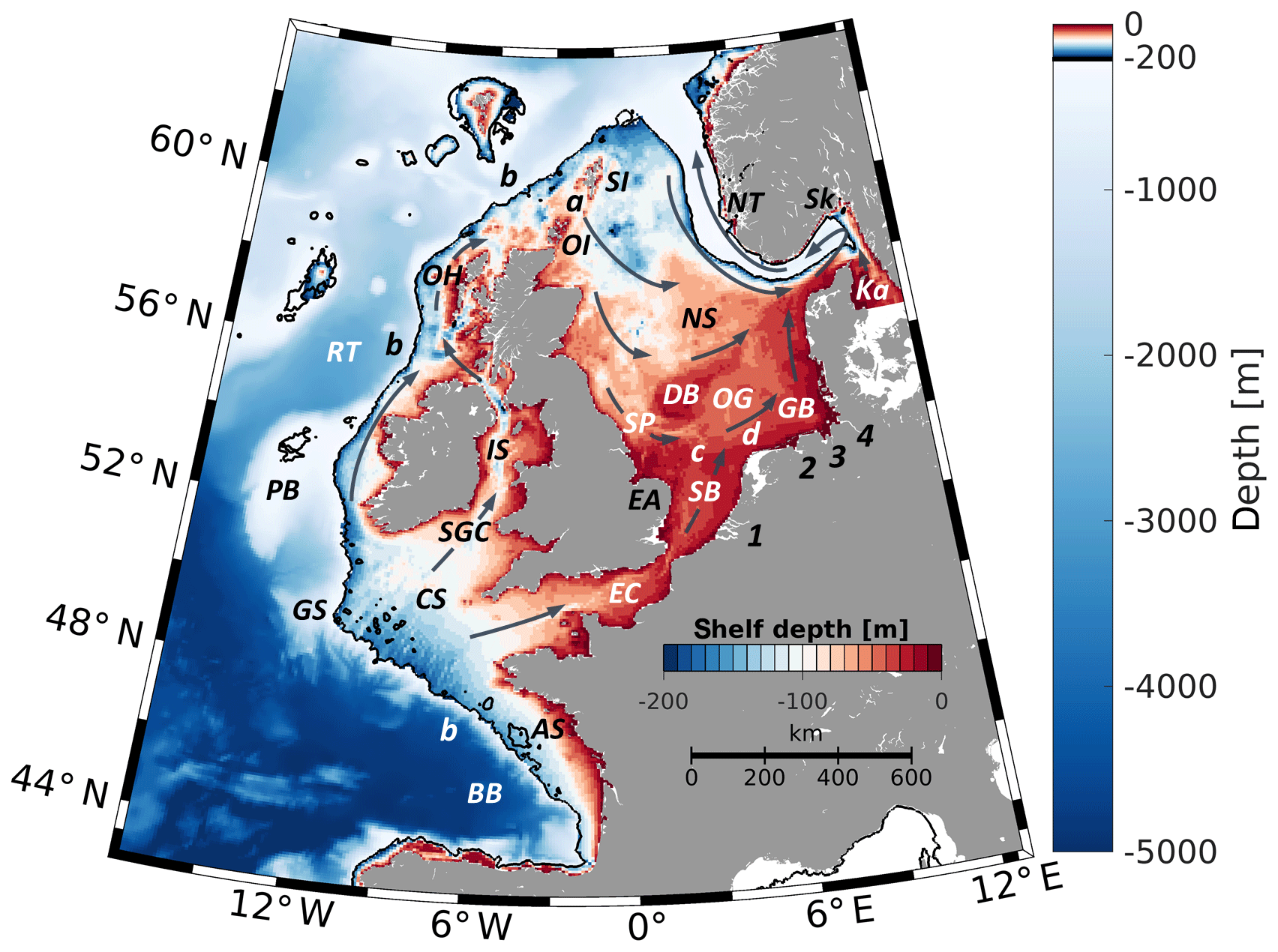
Figure 1Bathymetry of the model domain. The shelf is defined as depths shallower than 200 m (colour bar within the map). In this and all following figures, the 200 m depth contour is highlighted with a black solid line. Grey arrows schematically show the general shelf sea circulation. The abbreviations used in the text are as follows: Armorican Shelf (AS), Bay of Biscay (BB), Celtic Sea (CS), Dogger Bank (DB), East Anglia (EA), English Channel (EC), German Bight (GB), Goban Spur (GS), Irish Sea (IS), Kattegat (Ka), North Sea (NS), Norwegian Trench (NT), Oyster Ground (OG), Outer Hebrides (OH), Orkney Islands (OI), Porcupine Bank (PB), Rockall Trough (RT), Skagerrak (Sk), Southern Bight (SB), St. George's Channel (SGC), Shetland Islands (SI), Silver Pit (SP), Fair Isle Current (a), European Slope Current (b), East Anglia Plume (c), Frisian Front (d), Rhine (1), Ems (2), Weser (3), and Elbe (4).
In the following, we briefly summarise some basic oceanographic knowledge about the ENWS (the study area is shown in Fig. 1). The slope current dynamics and exchanges between the deep ocean and shelf have been analysed by Huthnance (1995), Davies and Xing (2001), Huthnance et al. (2009), and Marsh et al. (2017); Lagrangian drifter experiments in this area have been described by, for example, Booth (1988) and Porter et al. (2016). The prevailing westerlies induce on-shelf water transport from the Celtic Sea up to the Outer Hebrides (Huthnance et al., 2009). Water entering the Celtic Sea flows into the English Channel, into the Irish Sea via St. George's Channel, or around the southwest of Ireland (grey arrows in Fig. 1 schematically show the principal shelf circulation). The water exiting the Irish Sea flows around the Outer Hebrides and joins the on-shelf transported water. Part of this water enters the North Sea, mainly via the Fair Isle Current, where it begins an anticlockwise journey through the North Sea. The third path of waters entering the North Sea originates from the Baltic Sea; subsequently, those waters are integrated into a complex system of currents in the Skagerrak and the Norwegian Trench. In this area, the Atlantic and Baltic Sea waters undergo strong mixing. Along the southern slope of the Norwegian Trench, a branch of the European Slope Current flows toward the Baltic Sea, while a current flowing in the opposite direction follows the northern slope of the trench. In addition, large river runoff influences the water masses in the North Sea and along the Scandinavian coast, explaining the low salinity along coastal areas. Further details of the North Sea circulation can be found in, for example, Howarth (2001) and in the above-mentioned reviews. The major hypothesis in the present study is that although the North Sea is very shallow, it contains an important vertical circulation. Revealing such characteristics is the first specific objective of the present study.
Much is known about the thermohaline fronts on the ENWS and its estuaries (Simpson and Hunter, 1974; Hill et al., 2008; Holt and Umlauf, 2008; Pietrzak et al., 2011). Although large parts of this ocean area are vertically well mixed, seasonal and shorter-term variability lead to pronounced differences in the positions and strengths of the fronts. Freshwater fluxes are also important, particularly in shallow coastal areas. Krause et al. (1986), Le Fèvre (1986), Belkin et al. (2009), Lohmann and Belkin (2014), Mahadevan (2016), and McWilliams (2016) addressed the biological consequences of frontal systems, and the frontal physics are summarised in Simpson and Sharples (2012). However, to the best of the authors' knowledge, the frontal dynamics of the ENWS have not been addressed from a Lagrangian perspective; therefore, this will be the second specific objective of our study.
Most previous studies that employed Lagrangian particle tracking in the region of the ENWS (Backhaus, 1985; Hainbucher et al., 1987; Schönfeld, 1995; Rolinski, 1999; Daewel et al., 2008; Callies et al., 2011; Neumann et al., 2014; Marsh et al., 2017) addressed only part of the region studied herein. Hence, our overall objective is to provide a comparison among the specific hydrodynamic regimes in different areas of the ENWS and exchanges between these areas. One example has been recently provided by Marsh et al. (2017) for part of the European Slope Current. Lagrangian approaches applied to other ocean regions can be found in Bower et al. (2009) for the North Atlantic, Paparella et al. (1997) for the Antarctic Circumpolar Current, Reisser et al. (2013) for Australia, van Sebille et al. (2015) for the world ocean, Maximenko et al. (2018) for tsunamis, and Froyland et al. (2014) and van der Molen et al. (2018) in terms of connectivity studies.
The present study was initiated in the framework of a project studying the fate of marine litter in the North Sea (Gutow et al., 2018; Stanev et al., 2019). Here, we extend the area of our analyses to include the entire ENWS, the European Slope Current, the Bay of Biscay, and parts of the northeast Atlantic. Unlike our recent studies, herein we address virtual Lagrangian particles (“particles” in the following) and not real drifters. These particles are transported only by 3-D ocean currents (turbulence, Stokes drift, and wind drag are not considered). Thus, this study aims at giving a Lagrangian representation of the velocity field of the ENWS and the surrounding deep ocean.
In Sect. 2, we will describe the model, its setup, and the Lagrangian experiments. In Sect. 3.1 and 3.2, Eulerian model results and model validations are presented followed by Lagrangian model results and sensitivity experiments being discussed in Sect. 4.1 to 4.5. The paper ends with a brief conclusion in Sect. 5.
2.1 The numerical model
The Nucleus for European Modelling of the Ocean (NEMO) hydrodynamic ocean model is used in this paper (Madec, 2008). For this study, the Atlantic Margin Model configuration with a 7 km resolution (AMM7; Fig. 1) of NEMO is chosen because it appears to be one of the best validated model setups for the ENWS (O'Dea et al., 2012, 2017). The numerical model solves the primitive equations using hydrostatic and Boussinesq approximations. The horizontal resolution is 1∕9∘ in the zonal direction and 1∕15∘ in the meridional direction; that is, the resolution is approximately 7.4 km. This lateral resolution allows for resolving, for example, tidal mixing fronts, modification of tidal ellipses by stratification, strong shear stresses induced by tides, and eddies with diameters larger than 30–40 km. Not fully resolved are, for example, frontal jets and shelf break downwelling (Stanev and Ricker, 2020). There are 297×375 grid points altogether and 51 vertical σ layers. For tracer, i.e. temperature and salinity, advection, we employ the total variation diminishing (TVD) scheme; diffusion takes place on geopotential levels with a Laplacian operator (the constant horizontal eddy diffusivity is specified as 50 m2 s−1). For momentum diffusion, a bi-Laplacian scheme is applied to act on the model levels (constant coefficient of m4 s−1). The generic length scale (GLS) k–ε scheme is used as the turbulence closure scheme; the bottom friction is non-linear with a log-layer structure, a roughness length of m, and a drag coefficient range of to . The baroclinic time step is 300 s. The output, including the salinity (S), temperature (T), velocities (u, v), and sea surface height (SSH), is written hourly.
The atmospheric forcing is provided by the UK Met Office’s numerical weather prediction (NWP) model with a 3 h temporal resolution for the fluxes and an hourly resolution for the 10 m wind and air pressure. The model uses climatological river runoff based on the European HYdrological Predictions for the Environment (E-HYPE) product of the Swedish Meteorological and Hydrological Institute (SMHI). The open boundary forcing has two parts: a tidal harmonic signal (15 constituents Q1, O1, P1, S1, K1, 2N2, MU2, N2, NU2, M2, L2, T2 ,S2, K2, M4) and the remaining barotropic part consisting of the sea surface elevation and depth-mean currents (2-D surge component). The barotropic forcing was implemented following the Flather radiation scheme (Flather, 1994). In addition to tidal harmonic forcing, tidal potential forcing using the same tidal constituents was applied over the entire model area. The initial and boundary data for temperature and salinity were taken from the operational Forecasting Ocean Assimilation Model (FOAM) AMM7 setup. Further details about the model setup are given in Stanev and Ricker (2020), where the same model configuration has been first used. The period of integration considered here spans from 1 January 2014 to 31 December 2015 of which the first year is the spin-up period. The analyses of the results are performed for the area between 42.57–63.50∘ N and 17.59∘ W–13.00∘ E, which is slightly smaller than the model domain to avoid effects due to the open boundaries.
Although part of this study could be performed using the freely available operational FOAM AMM7 data, we run the above-mentioned model to (1) perform Lagrangian simulations online, (2) take into account timescales shorter than days, and (3) carry out some additional sensitivity experiments. In contrast to the operational FOAM AMM7 model setup, the data are not assimilated here. In the following, the basic experiment is referred to as the control run (CR). In one sensitivity experiment, the tides are turned off; this experiment is referred to hereafter as the non-tidal experiment (NTE). In two other sensitivity experiments, the wind forcing is low-pass filtered with a moving time window of 1 week (referred to as the filtered-wind experiment, FWE) or completely turned off (the non-wind experiment, NWE). The changes in the model forcing are applied on 1 January 2015.
2.2 Validation data
For validation of sea surface temperature (SST), data from the Operational Sea Surface Temperature and Ice Analysis (OSTIA) system are used, which provides a gap-free synthesis of several satellite products (Donlon et al., 2012). Velocities have also been validated using nine passive GPS surface drifters; these drifters provide the most appropriate type of in situ data for validating the model's ability for particle advection. The drifter design and a bottom-mounted sail reduce the effect of direct wind drag (see Callies et al., 2017, for a technical description of the drifters). The drifters were released in the German Bight during RV Heincke cruise HE445, and their position was sent every ∼20 min from May to July 2015. The dataset is freely available (Carrasco and Horstmann, 2017) and, to the best of the authors' knowledge, it is the only GPS drifter dataset available for the ENWS during the period of the simulations analysed herein. For validation, the model velocities are interpolated to the drifter positions in space and time. Drifter velocities are also compared with independent observations using high-frequency (HF) radar data. The HF radar system described by Stanev et al. (2015) and Baschek et al. (2017) consists of three measurement stations covering most of the German Bight and measures ocean surface velocities.
2.3 Particle release experiments
Particles are released in the hydrodynamic model, and their propagation is used to analyse the transport properties. The experiments were carried out “online”; that is, the particle trajectories were computed within the hydrodynamic model at every time step. Additional experiments were carried out “offline” using the model velocity output. High-frequency processes and vertical transport are better accounted for in the former experiments, whereas backtracking is only possible offline. An intercomparison between the online and offline integrations using the same particle setup demonstrated that neither approach leads to drastic differences when comparing 2-D horizontal particle transport properties.
The online advection of particles was achieved by the freely available open-source ARIANE model. The version of ARIANE implemented in NEMO has frequently been used in other studies, e.g. Blanke and Raynaud (1997) and Blanke et al. (1999). Further details of the ARIANE model can be found in the appendix of Blanke and Raynaud (1997) and in the ARIANE user manual (http://stockage.univ-brest.fr/~grima/Ariane/, last access: 5 July 2019). Beaching is not possible; that is, the total number of particles remains constant over time. An extra wind drag is not used and neither is additional horizontal and vertical diffusion for the particles (pure Lagrangian particles). Actually, velocity gradients together with a small advection time step (van Sebille et al., 2018) provide a sufficiently high shear diffusion. The vertical velocity is taken into account and the particle positions are written hourly. Particles are neutrally buoyant and provide a Lagrangian representation of the velocity field.
Table 1Summary of the particle release experiments; further details are given in Sect. 2.3. Surface release is done at 1 m depth and bottom release one grid cell above the sea floor. Particle release was done once at the beginning of the respective month in 2015.

Different seeding strategies were implemented. In one class of experiments (no. 1–4 in Table 1), the particles were seeded laterally at 1 m (surface particles), as well as in the grid cells just above the seafloor (bottom particles) over the whole domain. In the second experiment (no. 5 in Table 1) named CR-B, the particle tracking process was carried out offline. For this purpose, the freely available open-source model OpenDrift (Dagestad et al., 2018) was used, in which the particles were advected by a second-order Runge–Kutta scheme. The offline calculation was performed backward in time at a constant depth with a velocity input time step, a model time step, and an output time step of 1 h. The particle release depth in this experiment was 1 m. In a third experiment (no. 6 in Table 1) named CR-V, particles were released in a 100 km wide strip extending oceanward from the 150 m isobath starting in the Bay of Biscay and ending north of the Shetland Islands at 61.7∘ N (red and blue coloured area in Fig. 9a–d). In this experiment, particles were seeded vertically every 20 m; this is exemplarily shown for the depth 900–1000 m in Fig. 9e.
The seeding strategy was consistently executed as follows. The initial distribution of particles was uniform with 1 particle per model grid cell; that is, 64 831 particles per depth layer for the whole domain (experiment nos. 1–5 in Table 1) and a total of 345 011 particles in experiment no. 6. In CR and CR-V (experiment nos. 1 and 6, respectively), particle release was repeated on the first day of every month in 2015, and particles were traced for 1 month. Thus, 12 datasets, each including 1 month of trajectory data, were generated. Additionally, for the seeding in January, the particle positions were traced for 6 months. The FWE, NWE, and CR-B (experiment nos. 3–5, respectively) were conducted only for January 2015, whereas the NTE (experiment no. 2) was additionally run for July 2015.
Experiment no. 1 aims to understand and visualise the general circulation of the ENWS at both the surface and bottom. The uniform initial distribution of particles enables a comprehensive Lagrangian representation of surface and bottom dynamics over the whole domain. This experiment will also be used to analyse accumulation and dispersal areas as well as vertical dynamics and frontal effects. Further, it serves as the reference run for the sensitivity experiments. The sensitivity experiments (experiment nos. 2–4) are performed to assess the influence on Lagrangian dynamics of some of the most important drivers for particle advection, i.e. tides and wind. Experiment no. 5 supports the analyses of vertical shelf dynamics and complements experiment no. 1. Experiment no. 6 provides a 3-D particle seeding along the continental slope to study the dynamics there.
2.4 Normalised cumulative particle density
The analyses of the results will focus on typical Lagrangian properties, e.g. the positions of the particles and their trajectories. Such a presentation could be considered inferior compared with the Eulerian presentation, which displays the concentrations of properties. However, from these Lagrangian characteristics, one can derive properties similar to the concentration that can represent the “compaction” process of particles in certain areas or identify the areas that are more frequently visited by the particles. These properties related to particle density allow the areas in which particles accumulate to be identified.
Different approaches to quantify particle accumulation have been proposed (Koszalka and LaCasce, 2010; Koszalka et al., 2011; van Sebille et al., 2012; Huntley et al., 2015). Below, in addition to the typical Lagrangian properties, a property named the “normalised cumulative particle density (NCPD)” is introduced that measures the number of particles that have visited each grid cell during a certain time interval. This quantity is normalised by the corresponding number of initial particles in the respective NCPD grid cell for the same time interval (in our case 1 particle per grid cell), which corresponds to a motionless situation:
where NCPD is the normalised cumulative particle density; (X, Y) represents the coordinates of an arbitrary grid cell in longitudinal and latitudinal directions, respectively, with dimensions dX and dY; n is the number of time steps from t0 to tn; u is the velocity field; and N is the number of particles at time step i in grid (X, Y). In the present study, (dX, dY) represents the model grid dimensions (dx, dy), but they could be larger or smaller for other applications. A NCPD greater (smaller) than unity corresponds to more (fewer) particles, which are identified in a grid cell, on average, than there would be without currents. Thus, the NCPD can be interpreted as the percentage of the initial number of particles averaged over time or as proportional to the inverse residence time.
The definition of the NCPD is not straightforward if the initial particle concentration is zero in some areas. Further, if the number of particles in some areas remains small (e.g. areas close to an inflow-dominated open boundary or divergence zones), the statistical confidence of this property cannot be ensured. Therefore, areas where the NCPD is less than 30 % are excluded from the analysis (white areas in the following figures). In the present study, the focus will be on monthly timescales (tn=1 month). Choices of (dX, dY) and of the particle seeding have been made accordingly. For comparison, for integration times longer than 1 month, large areas remain free of particles; integration times shorter than 1 month would cause rather noisy results.
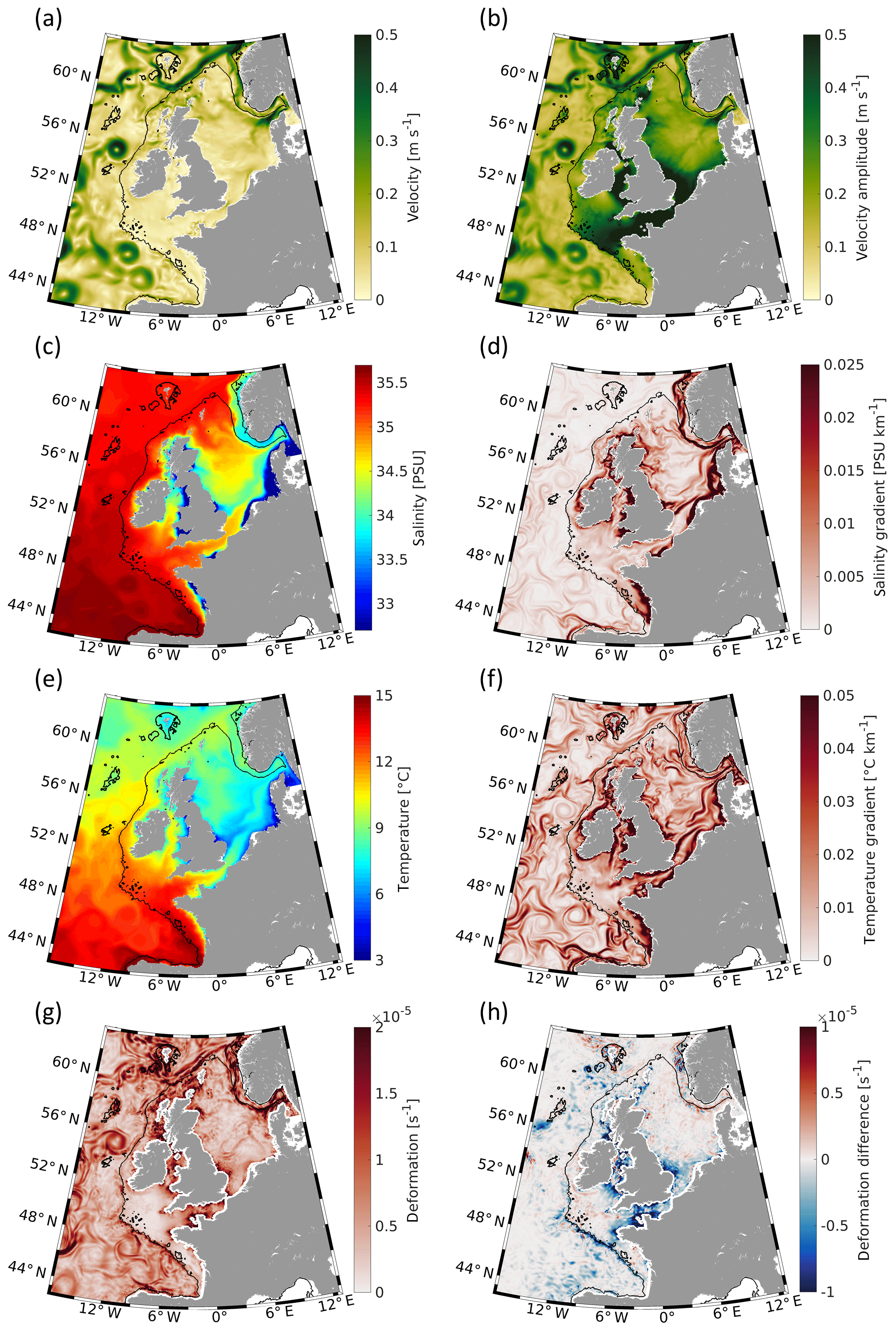
Figure 2Simulated surface properties in the control run (CR, no. 1; see Table 1) for January 2015: (a) velocity magnitude derived from the averaged u and v velocity components, (b) mean velocity magnitude, (c) mean salinity, and (e) mean temperature. Magnitudes of the (d) temperature and (f) salinity gradients as well as (g) the deformation in the CR and (h) the differences of the non-tidal experiment (NTE, no. 2) minus CR of the deformation are presented as 24.84 h averaged fields on 15 January 2015.
3.1 Analysis of the simulated dynamics
The circulation of the CR is very diverse in different model areas, but the differences among the dynamic regimes in the CR are most pronounced between the deep ocean and the shelf. The residual velocities (U) and velocity amplitudes for January 2015 (Fig. 2a, b) show basically two regimes: an eddy-dominated regime west of the continental slope and a tidally dominated regime on the shelf. The latter is characterised by relatively low residual velocities (Fig. 2a) and large velocity oscillations in the English Channel, Southern Bight, Irish Sea, and Celtic Sea (Fig. 2b). The transition between these two regimes occurs along the 200 m isobath, which can be considered a separation line between the dynamics of the shelf and deep ocean. A sequence of mesoscale eddies is developed offshore of the western shelf edge with a dominant one in the Rockall Trough (Fig. 2a, b), which is also readily visible in the corresponding SSH pattern (not shown). The largest amplitudes of the sea level oscillations are observed around the British Isles, in the English Channel, and in the German Bight. The dominant wind direction is from the west due to the prevailing westerlies (Fig. S1 in the Supplement).
The simulated thermohaline characteristics are consistent with the existing knowledge: the coastal waters, particularly those in the German Bight, are less saline (Fig. 2c) and represent typical regions of freshwater influence (ROFIs). In the German Bight, most of the low-salinity water originates from the Rhine, Ems, Weser, and Elbe rivers and spreads along the German and Danish coasts before it reaches the Skagerrak, where it mixes with the low-salinity outflow from the Baltic Sea. The pattern of the salinity gradient (Fig. 2d) reveals features along the coasts and at the major fronts in the German Bight. Additionally, the two current branches in the Norwegian Trench associated with two opposing flows (one flowing to the east along the southern slope and another flowing in the opposite direction along the northern coast) are also easily observed as areas characterised by large salinity gradients.
In January, the overall temperature distribution is characterised by cold temperatures on the shallow shelf and a south–north temperature gradient in the deep water south of Ireland (Fig. 2e). A warm water plume exits the English Channel (Fig. 2e) and traces the pathway of warm Atlantic water into the North Sea, which is also known from satellite observations (Pietrzak et al., 2011). At the northern boundary of this plume, the East Anglia Plume is known to transport suspended particulate matter (SPM) to the northeast. Along with a second plume extending into the Irish Sea, these plumes are visible as strong temperature gradients (Fig. 2f). The temperature gradient also reveals a number of mesoscale features occurring in the deep ocean along the rims of currents (compare Fig. 2f with 2a). In July, the warmest temperatures can be found in the Bay of Biscay and along the coasts of the shallow shelf, especially on the Armorican Shelf (Fig. S2a). The July temperature distribution is also characterised by well-pronounced temperature gradients, e.g. the Frisian Front located somewhat north of the Dutch coast. The simulated gradients along the Celtic Sea Front, Ushant Front, Islay–Malin Head Front, and the Flamborough Head Front (black circles in Fig. S2a) support the results by Pingree and Griffiths (1978). The disappearance of these fronts in the results of the NTE demonstrates that they are tidal mixing fronts (see Fig. S2a, b). Overall, Fig. 2a–f support much of what is known from previous studies about the general dynamics and thermohaline characteristics of the ENWS (e.g. Pätsch et al., 2017).
Understanding the differential properties of currents is of utmost importance to understand the propagation of Lagrangian particles. Therefore, we will present a brief analysis of deformation, as proposed by Smagorinsky (1963):
with horizontal tension strain,
and horizontal shearing strain,
with (u, v) being the model velocities components and (∂x, ∂y) the model grid size in longitudinal and latitudinal directions, respectively. Figure 2g shows the 24.84 h averaged (two M2 cycles) deformation obtained from the CR surface currents on 15 January 2015 (the influence of the most dominant tidal constituent is excluded). The order of this property, O (10−5), is within the ranges measured by Molinari and Kirwan (1975) with Lagrangian drifters in the Caribbean Sea. The most obvious features are the two large areas on the shelf exhibiting low deformation, namely the North Sea and the Celtic Sea, including the Armorican Shelf connected by the English Channel and Southern Bight, where several localised high-deformation areas appear (compare Fig. 2g with 2b). High-deformation areas are also present in the Irish Sea extending to the northern coast of Ireland. The difference of deformation between the NTE and CR (i.e. NTE minus CR) clearly shows the impact of tides on these three areas (Fig. 2h). In addition to shallow, enclosed areas, the deformation along the shelf edge of the Celtic Sea is also affected by tides. High-deformation features in the deep ocean arise at the eddy boundaries (compare Fig. 2g with 2a) and most of them are also present in the NTE. Hence, flow deformation is expected to be of significant importance for water masses in the deep ocean. Exceptions are the Bay of Biscay and the northwest of the domain where the deformation is less pronounced in the NTE. The difference patterns (Fig. 2h) there have scales of mesoscale eddies suggesting that these eddy dynamics could be coupled to the one of tides. In the Norwegian Trench, high deformation is observed along the southern 200 m isobath. Here, the influence of tides arises as small-scale patterns associated with the interaction of the two currents.
3.2 Model validation
The root-mean-square difference of January 2015 SST of the model and OSTIA data reveals values smaller than 1.5 ∘C in vast areas of the model domain, whereas values between 0.5 and 1.0 ∘C are the typical range (Fig. S3).
Scatter plots of drifter and model velocities show a good model performance in the range of ±25 cm s−1, where the quantile–quantile plot (QQ plot) is almost along the diagonal (Fig. S4a and S4b). Deficiencies in the model occur at higher velocities, where the model is too slow probably due to the neglected direct wind drag and Stokes drift (Röhrs et al., 2012; Stanev et al., 2019). Nevertheless, the linear correlations of the u and v velocity components of 0.88 and 0.84, respectively, between the drifters and the model and the corresponding root-mean-square errors (RMSEs) of 14.3 and 12.4 cm s−1 are considered to reflect a satisfactory model performance (Table 2).
Table 2Summary of the model velocity validation performed by comparing GPS drifter velocities with the CR and HF radar velocities; the surface velocity components of the latter were interpolated to the drifter velocities. Details are given in the text. A positive bias denotes that drifter velocities are larger than the velocities of the CR or HF radar. The corresponding scatter plots are given in Fig. S4. n is the number of observations.
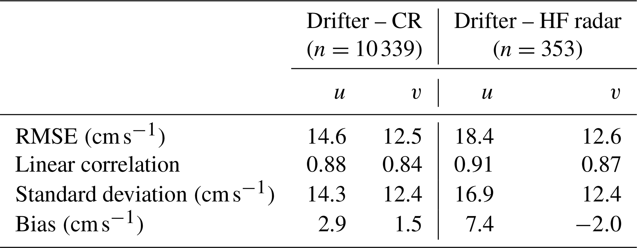
The quality of the above numbers illustrating the model skill can be better understood if the drifter data are compared with independent observations using HF radar data. The corresponding scatter plots (Fig. S4c and S4d) do not show as much underestimation of high velocities as in the model (compare with Fig. S4a and S4b), but the spread of the data is comparable to the case of the model–data comparison (the standard deviation between the two observations is even larger than in the case of the model–data comparison). The conclusion from Table 2 is that the difference between the estimations from the model and data are not larger than that between two observations. Similar validations provided by Stanev et al. (2019) for the North Sea also demonstrate the credibility of the Lagrangian tracking approach.
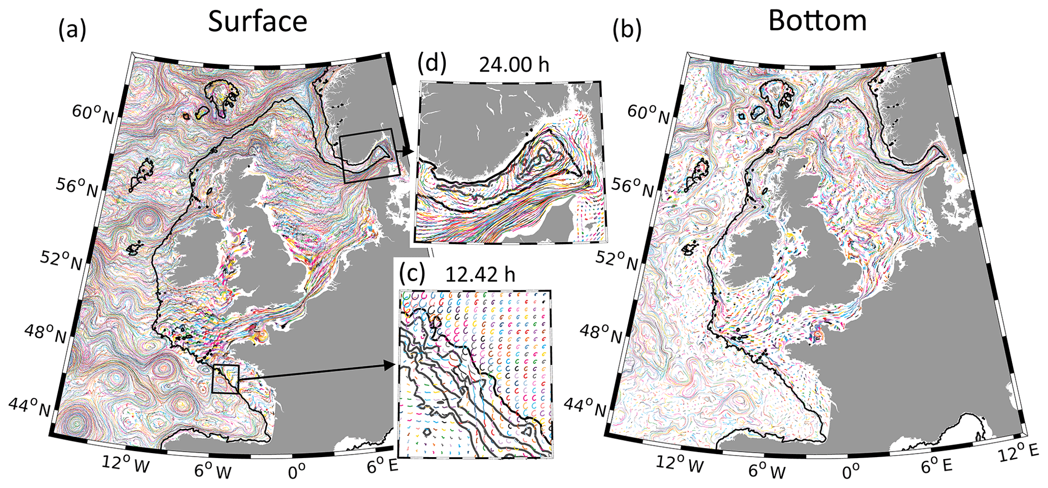
Figure 3Lagrangian trajectories of every eighth particle after 15 d of integration in the control run (CR, no. 1; see Table 1) released on 1 January 2015. Particles are released at (a) the surface and (b) bottom. Panels (c) and (d) are magnified views of the domain showing all trajectories of (c) the first 12.42 h and (d) 24.00 h representative of different dynamics: (c) the area of the Armorican Shelf continental slope including tidal ellipses and (d) the circulation in the Skagerrak. The trajectory colours are randomly chosen for better visibility. Grey lines are isobaths in (c) 800 m and (d) 200 m steps.
4.1 Overall analysis of trajectories and particle dynamics
The particle trajectories (Fig. 3) of the CR (experiment no. 1; see Table 1) show the well-known dynamic features of the ENWS and the surrounding deep ocean. In relatively shallow areas, e.g. the English Channel, Southern Bight, and Irish Sea, the surface and bottom currents are almost parallel (Fig. 3a, b). This is typical for tidally influenced wind-driven shallow water circulation. Trajectories symbolising currents appear relatively thick in the areas dominated by strong tides because the large-scale presentation cannot effectively resolve small tidal excursions. This is supported by the magnified representation of the dynamics in Fig. 3c and d. After 12.42 h, the trajectories on the shelf present as nearly closed circles. The difference between the start and end positions on the circular loops give an estimate of the net transport, which is much smaller than the tidal excursions. The net transport rapidly increases, and the tidal excursions decrease further off-shelf beyond the 800 m isobaths, where the mesoscale dynamics are dominant. As in the case of the Eulerian visualisation of the velocity field, the 200 m isobath can be considered the boundary separating the dynamics of the shallow and deep ocean. The meandering of the European Slope Current along the shelf edge (at ∼500–2000 m) is pronounced from the Bay of Biscay to the Goban Spur and around the Porcupine Bank (Fig. 3b). The Skagerrak and Norwegian Trench also show pronounced mesoscale dynamics (Fig. 3d).
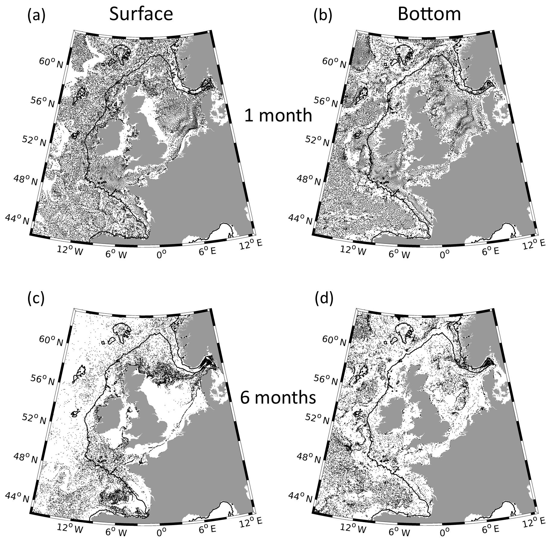
Figure 4Particle positions after (a, b) 1 month and (c, d) 6 months released on 1 January 2015 at (a, c) the surface and (b, d) bottom in the control run (CR, no. 1; see Table 1).
4.2 Surface and bottom patterns of the particle distribution
Despite some similarities between the surface and bottom trajectories (Fig. 3), the particle accumulation patterns in shallow areas are considerably different (Fig. 4). To investigate these differences, the positions of the particles released in January (CR, experiment no. 1; see Table 1) are displayed in Fig. 4. After 1 month, the surface-released particles accumulate mainly along narrow patterns on the shelf and in the Skagerrak (Fig. 4a). In contrast, the coastal regions around Great Britain and Ireland (but also in the German Bight) can be considered divergence zones. The particle distribution in the deep ocean also shows small strip-type patterns, especially in the southwestern part of the model domain, and will be discussed in detail later (see Sect. 4.3). In the following, examples of pronounced accumulation and dispersal features are given.
There is a tendency for the bottom-released particles to leave areas with a steep bottom slope. The most obvious example is the continental slope along the 200 m isobath from the Spanish coast around the Goban Spur and Porcupine Bank (Fig. 4b) until the Norwegian Trench. Van Aken (2001), Huthnance et al. (2009), and Guihou et al. (2018) demonstrated that slope currents, downward flows of shelf water, and internal waves, respectively, dominate the dynamics of the ENWS continental slope. These processes can induce a net transport and in turn a tendency of bottom-released particles to leave the continental slope.
After 6 months, vast areas of the shelf and the western part of the domain become free of particles. The particles flow from the English Channel along the Frisian Front in the south and the Fair Isle Current in the north into the inner North Sea (Fig. 4c). The pattern in the Irish Sea is similar to the Frisian Front: a narrow strip of particles in the middle of this basin is the remnant of a similar strip from an earlier time (Fig. 4a) connecting the source of particles (in the south) to their sink (in the north). The region around the Orkney and Shetland islands accumulates particles owing to on-shelf transport by the westerlies, which also drives particles away from the western open boundary. This region additionally receives particles from the south originating from the Irish Sea or floated around the western coast of Ireland; in both cases, these particles are sourced from the deep ocean. Likewise, the Bay of Biscay accumulates particles on timescales of several months. Bottom accumulation on the shelf occurs mainly west and south of the Dogger Bank (Fig. 4d). Also the bottom trajectories (Fig. 3b) show that particles north of Dogger Bank are forced to flow around its western edge through the Silver Pit into the Oyster Ground (see the bathymetry in Fig. 1) suggesting topographically influenced particle motions. Once the particles reach this basin, they can flow out only northward along its thalweg until they reach the northeastern edge of Dogger Bank (compare Fig. 4d with Fig. 1).
In the Skagerrak, the situation is as follows. At the bottom, the Norwegian Trench supplies the Skagerrak with particles from the Atlantic along its southern slope. At the surface, the Skagerrak receives particles from the Fair Isle Current, the German Bight, and the Baltic Sea. Particles approaching the Skagerrak can become trapped in its circular and eddy-dominated velocity pattern (Figs. 3d and 2b), which extends from the surface down to the bottom (see also Rodhe, 1987; Gutow et al., 2018). In the Norwegian Trench, the particle distribution has high spatial variability due to the irregular mesoscale dynamics.
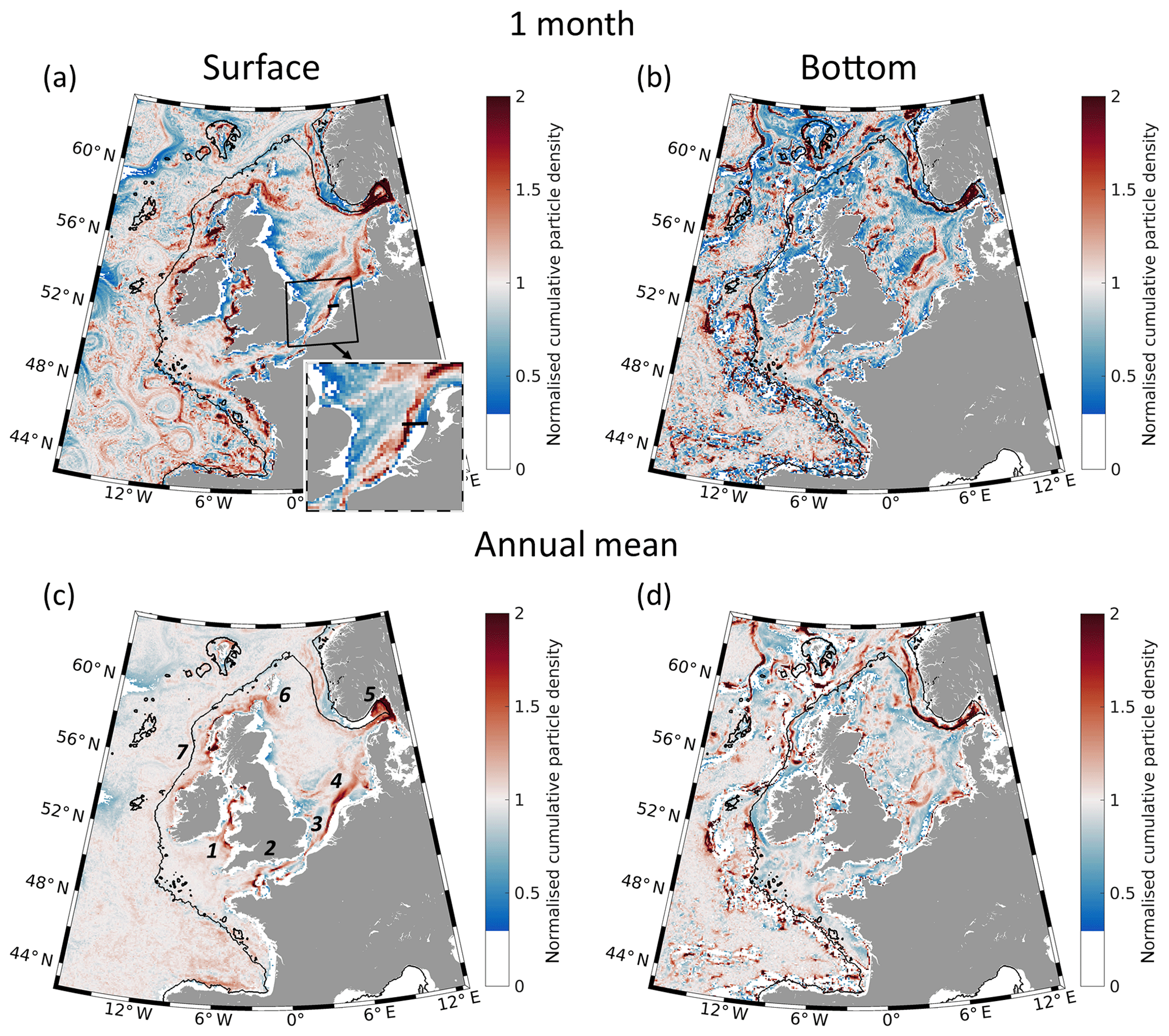
Figure 5Tendencies of accumulation shown as (a, b) the January mean normalised cumulative particle density (NCPD) and (c, d) the average of monthly NCPD for 2015 (averages of Figs. S5 and S6, respectively) in the control run (CR, no. 1; see Table 1). Panels (a) and (c) correspond to surface-released particles, while panels (b) and (d) correspond to bottom-released particles. In (a), the solid black line located in the Southern Bight is the transect shown in Fig. 7 (enlarged in the inset). The numbers in (c) indicate the most pronounced accumulation areas.
4.3 Tendencies of particle accumulation
The instantaneous particle positions are not sufficiently representative of their accumulation and dispersal over long periods, and this can lead to misinterpretations of their accumulation trends. This becomes evident by comparing the particle positions after 1 month (Fig. 4a, b) with the NCPD for the same period (Fig. 5a, b). Although the general surface and bottom particle patterns (Fig. 4a, b) for January 2015 are comparable to the mean accumulation patterns (Fig. 5a, b), some features do not coincide. The monthly NCPDs for all 12 months are shown in Figs. S5 and S6 for the surface- and bottom-released particles, respectively. At the surface, only a few accumulation areas are visible on the annual mean map (numbered red areas in Fig. 5c); these areas are located in the Irish Sea (1), English Channel (2), Southern Bight (3), German Bight (4), Skagerrak (5), at the Fair Isle Current (6), and at the northern coasts of Ireland and Great Britain (7). Vast coastal areas have a NCPD smaller than 0.3, implying offshore propagation. Despite the numbered accumulation areas and coasts prone to particle removal, most of the domain shows neither particle accumulation nor removal (NCPD≈1).
At the bottom, particle accumulation is highly variable in the deep ocean, but the removal of particles from areas with steep topography is evident (Fig. 5d). On the shelf, the tendency of particles to propagate away from coasts is smaller than for surface particles; particles even accumulate, e.g. in the German Bight and along the eastern British coast (discussed in detail in Sect. 4.4). Further, accumulation takes place south of Dogger Bank and in the Skagerrak. It is worth noting that the major accumulation pattern at the surface along the Frisian Front (3 and 4 in Fig. 5c) has as its counterpart a pattern of removal at the bottom (compare Fig. 5c and 5d). Additionally, coastward of accumulation area 4, there is a removal area at the surface; in the same area, the bottom pattern shows a tendency for accumulation. These opposite tendencies in the surface and bottom layers suggest that the vertical circulation is also important in shallow environments. The inflow along the southern slope of the Norwegian Trench appears as increased particle accumulation.
There are some prominent small-scale features (strip-like or filament-like characteristics) in the deep ocean occurring as NCPD maxima and minima (Figs. 5a and S5) as well as particle accumulation and dispersal in the particle distribution (Fig. 4a). These features change their positions depending on mesoscale dynamics. They are reminiscent of the attributes reported by Haller and Yuan (2000), who demonstrated that particles initially located outside eddies accumulate in lines along the boundaries between them. When the averages are computed for a longer period, these filaments tend to disappear (compare Fig. 5a with 5c), which is explained by the fact that the timescales of eddy motions are substantially shorter than the annual scale. This follows from the changes in the position and occurrence of the strip-type areas with NCPDs greater than 1 from month to month (compare the results from single months of Fig. S5). A more profound Lagrangian representation of eddies and their coherent character can be found in, for example, Beron-Vera et al. (2019).
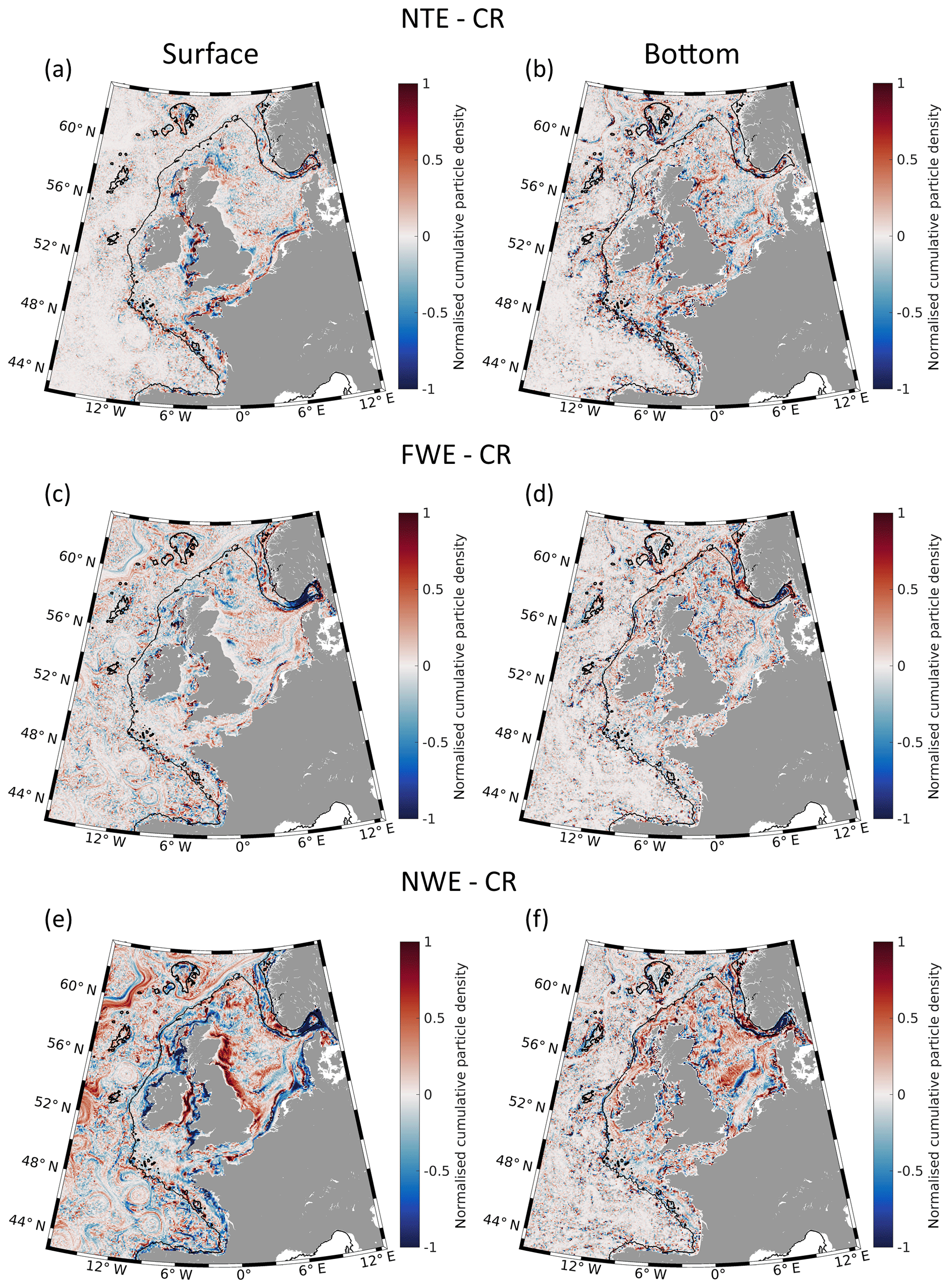
Figure 6Analysis of the sensitivity experiments with respect to tides and wind. Panels (a) and (b) are the differences of normalised cumulative particle density (NCPD) in the non-tidal experiment (NTE, no. 2; see Table 1) minus the control run (CR, no. 1) in January 2015 at (a) the surface and (b) bottom. Panels (c) and (d) are the corresponding differences between the filtered wind experiment (FWE, no. 3) and the CR; panels (e) and (f) are the differences between the non-wind experiment (NWE, no. 4) and the CR.
4.3.1 The role of tides
The difference in the January NCPDs between the NTE and CR (experiments nos. 2 and 1, respectively; see Table 1 and Fig. 6a, b) demonstrates that the tidal forcing considerably affects the accumulation patterns on the shelf. At the surface, the largest differences between the two experiments occur along the East Anglia Plume and Frisian Front and along the front in the Irish Sea (Fig. 6a). Obviously, the tidal signal affects frontal-like structures. Further differences between the two experiments appear in the English Channel, around the north of Great Britain and the Fair Isle Current, and at the continental slope of the Celtic Sea. In most of the remaining parts of the domain, these differences are rather small.
Nevertheless, tides also affect the accumulation of particles in the deep ocean, which is dominated by sub-basin-scale eddies, as well as other areas in the Bay of Biscay and in the Norwegian Trench and Skagerrak, which are dominated by mesoscale motions. This could serve as another indication of the interaction between tides and mesoscale dynamics.
The most pronounced large-scale feature in the differences observed at the sea surface is in the vicinity of the shelf (Fig. 6a). At the bottom (Fig. 6b), the largest differences between the two experiments occur also beyond the 200 m isobaths in the direction of the open ocean. The changing sign of the difference reflects large oscillations at small scales of O (grid size), possibly indicating that a further increase in the model resolution is needed to adequately resolve the accumulation and dispersion of particles in the area of the continental slope. Bottom patterns in the North Sea are also present and clearly demonstrate the importance of tides as a driver of particle accumulation there. The principal patterns are similar to the surface with differences around Great Britain but the difference signal is more variable. In the Southern Bight and southern North Sea the difference patterns are rather distinct and follow the flanks of the Dogger Bank and the East Anglia Plume. This comparison between the surface and bottom patterns indicates that, unlike the currents, which do not drastically change in the vertical direction in the shallow ocean, the accumulation of particles at the bottom is different from that at the sea surface. This suggests that the tides modify the particle accumulation patterns by the induced shear diffusion. This finding is supported by the influence of tides on surface deformation (compare Figs. 6a and 2h), the pattern of which partly coincides with the NCPD difference.
4.3.2 The role of wind
A large part of the variability of shelf dynamics is caused by atmospheric variability (mostly on synoptic timescales) (Jacob and Stanev, 2017); therefore, we will analyse the contributions of wind to the accumulation and dispersion of particles in the FWE and NWE (experiments nos. 3 and 4, respectively; see Table 1). It is worth noting that the ranges of the responses to wind variability are comparable to the responses to tides. The overall conclusion from the comparison among the differences in the surface properties between the NTE and CR (Fig. 6a) from one perspective and between the FWE and CR (Fig. 6c) from another perspective is that the largest differences caused by tides and winds occur in almost the same areas: the Frisian Front and Irish Sea Front, the continental slope, and the Norwegian Trench, whereas the English Channel is less influenced in FWE. Filtering the wind (FWE) also makes the accumulation strips “sharper”, whereas the short-term wind forcing tends to “blur” the particle distribution. However, turning the wind off (NWE) changes the accumulation patterns significantly (compare Fig. 6e and 6c). The most affected areas are (1) the coastal areas of Great Britain and Ireland; (2) the Skagerrak, which no longer accumulates particles; (3) the mouths of the Rhine and Elbe rivers, which extend further to the west; and (4) the coasts of the Armorican Shelf. Reducing the variability of the wind or turning it off completely also has very pronounced impacts on the bottom particles (compare Fig. 6d and 6f). The strongest impacts on bottom accumulation patterns are located in the northern part of the shelf and the Norwegian Trench and Skagerrak.
The difference between the FWE and NWE (not illustrated here) demonstrates that, on the shelf, the westerlies are essential for particle accumulation (compare Fig. 6c with 6e and Fig. 6d with 6f).
4.3.3 The role of fronts
The high-salinity and high-temperature gradients (fronts) in Fig. 2d and f are similar to the NCPD patterns shown in Fig. 5a. These fronts support the ones reported by Belkin et al. (2009), particularly the fronts in the southern North Sea. Additionally, in terms of the yearly averaged NCPD (Fig. 5c), the NCPD maxima coincide with the known front positions; in contrast, not all detected fronts show particle accumulation. There are also some differences from the analysis of Pietrzak et al. (2011), who analysed the dynamics of the Frisian Front and East Anglia Plume using satellite data of the SST and SPM. The differences between the present simulations and the results by Pietrzak et al. (2011) occur as a missing East Anglia Plume and are mostly because the particles in the model have a neutral buoyancy and because no particle sources are prescribed (the seeding is uniform).
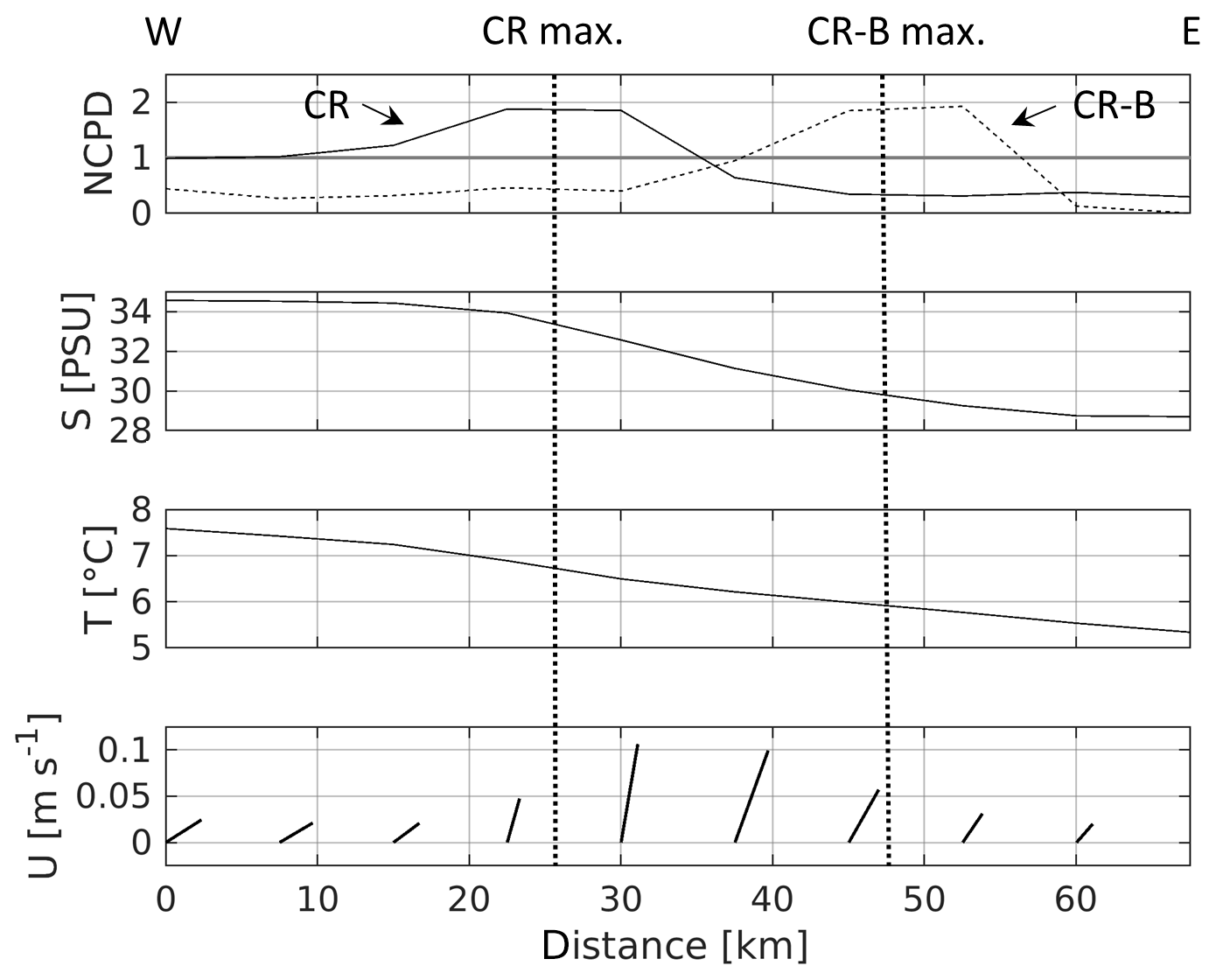
Figure 7Normalised cumulative particle density (NCPD), salinity (S), temperature (T) and residual velocity vectors (U) at the surface as the means of January 2015 along the transect in the Southern Bight (solid black line in Fig. 5a) in the control run (CR). The graph starts in the west and ends at the coast. The vertical dotted lines mark the NCPD maxima of the forward (left one, solid NCPD line) and backward (right one, dashed NCPD line) simulations (CR and CR-B, nos. 1 and 5, respectively; see Table 1).
To demonstrate the ability of a front to accumulate particles, a surface section across the Rhine Plume (Frisian Front) is chosen as an example (solid black line in Fig. 5a; see also its inset). The front separates the waters of the English Channel (higher salinity) and the Rhine ROFI (lower salinity). In Fig. 7, the graphs start in the west (left) and end in the east (right). The maximum NCPD in the CR (left vertical dashed line) is located where the salinity and temperature start to decrease (∼34.6 to 28.7 PSU (practical salinity units) and ∼7.6 to 5.3 ∘C, respectively). The related density changes are ∼4.62 and 0.28 kg m−3. Hence, the salinity causes the density gradient which in turn influences the accumulation of particles. In the backward simulation (CR-B; experiment no. 5; see Table 1), the NCPD maximum (right vertical dashed line) is at the same location with respect to the salinity change when the particles are coming from the opposite direction. Due to the residual currents, in the CR the particles come from the southwest and in the CR-B from the northeast. The peaks of the NCPD curves are bounded by a rather constant NCPD, which is higher on the side of particle supply than on the side of particle dispersion in the CR. In the CR-B, the particle supply is reduced by the front, because only particles from the German Bight and the Danish coastal region can reach the front. These regions are relatively small compared to the whole North Sea being the particle supplier in the CR. This implies that particle simulations in regions with frontal systems are not fully reversible and backward simulations have to be interpreted carefully. In terms of the position of NCPD maxima, the results of Fig. 7 are very similar to what has been found by Flament and Armi (2000) and Lohmann and Belkin (2014). Despite the vertical dynamics (see Sect. 4.4), particle accumulation along fronts can be explained considering that the residual velocity is not parallel to the front but oriented further clockwise (in the CR the orientation of the front is almost in the north–south direction, whereas U is veered clockwise). This would lead to a crossing of the front by particles, but the particles are hindered by the (haline) front and flow along it. In the CR-B, the dynamics are reversed and thus particles accumulate on the other side of the front. Particle accumulation along other ROFIs can also be observed at, for example, the western Danish coast along the Elbe river outflow. Postma (1984) called the boundary of the Wadden Sea a “line of no return” whose location is comparable to a strong salinity gradient (Fig. 2c, d). From the results of the present study, this interpretation of the boundary of the Wadden Sea can be confirmed: if a particle of the German Bight crosses the front, it is unlikely that it will be able to return.
In the NWE (Fig. 6e), the Frisian Front and Irish Sea Front are less pronounced than in the CR, demonstrating the intensification of frontal accumulation by wind. Due to the missing westerly wind, particles are no longer transported to the fronts, where they can accumulate in the areas of thermohaline gradients. This is especially true for regions where the wind is constantly blowing in the same direction, e.g. regions within the westerlies.
Another kind of shelf front is a tidal mixing front (Sect. 3.1 and Fig. S2), whose dynamics have been described repeatedly (e.g. Hill et al., 1993). These fronts are known to accumulate natural and artificial flotsam (Simpson and Pingree, 1978). In July, tidal mixing fronts are clearly visible as temperature gradients (Fig. S2a), and some of them can be observed in terms of NCPD patterns (Fig. S2c). In contrast to January, these fronts disappear in July if the tides are turned off and demonstrate their importance for particle accumulation in summer (Fig. S2d). Analyses of the January NTE results (not shown) show almost no vanishing NCPD maxima, implying that these maxima are not caused by tides. Due to the seasonal occurrence, tidal mixing fronts are less pronounced in the yearly averaged NCPD then other fronts, e.g. the fronts of ROFIs. However, not all of them occur as NCPD maxima. Although the well-known jet-like velocities along fronts can be seen in U in Fig. 7, the horizontal model resolution is probably too coarse; that is, the model cannot resolve all important frontal dynamics.
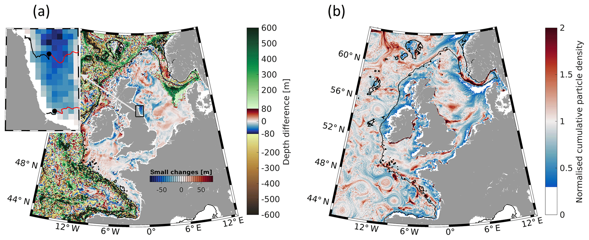
Figure 8(a) Difference of the final depth minus the initial depth of bottom-released particles after 1 month (January) in 2015 in the control run (CR, no. 1; see Table 1). Positive (negative) values indicate a depth increase (decrease). The model grid in which a particle was released is coloured depending on its depth change. The small figure shows a magnified view of the British coast with two exemplary bottom (black) and surface (red) trajectories starting at the big dots. The trajectories are detided with a 25 h moving average. (b) Tendencies of accumulation shown as the January mean normalised cumulative particle density (NCPD) calculated from the backward simulation (CR-B, no. 5).
4.4 Vertical circulation in the North Sea
Although shelf dynamics are dominated by strong horizontal motions, they cannot be considered fully two-dimensional. Examples of the role of vertical processes are given by tidal mixing fronts (Garrett and Loder, 1981; van Aken et al., 1987), upwelling in the German Bight (Krause et al., 1986), tidal straining (de Boer et al., 2009), and secondary circulation in estuaries. The differences between the surface and bottom accumulation patterns described in Sect. 4.3.3 (Fig. 5a, b) are indicative of the role of vertical processes. Such indications are clearly observed in the map of the differences between the vertical positions of particles released at the bottom after 1 month of integration (Fig. 8a). Pronounced depth changes appear along the eastern British coast, eastern Irish coast, around the Dogger Bank and in several smaller coastal areas, e.g. at the western French coast. Some of these patterns are topographically induced, like the one at the Dogger Bank, where particles from the northwest ascend and particles released on the Dogger Bank descend. However, a NCPD at the surface smaller than 1 and a NCPD at the bottom greater than 1 (compare Fig. 5c with 5d) suggest an upward movement of water not being induced by topography. Single-particle trajectories along the British coast reveal that the bottom flow is directed coastward and offshore at the surface (small inset in Fig. 8a).
In the backtracking experiment (CR-B, experiment no. 5; see Table 1; Fig. 8b), particles accumulate in coastal upwelling areas, emphasising the dynamics described above. The opposite situation is present on the northwestern Irish coast and in the western Irish Sea; here, a downward movement of water can be observed. The NWE shows that the prevailing westerlies are the main driver of coastal water transport at meridionally oriented coasts (Fig. 6e, f). Without wind, the eastern Irish and British coasts have NCPD values clearly exceeding 0.3; with the original wind forcing, these areas have NCPD values smaller than 0.3. In contrast, the NCPD of the western Irish coast and in the western Irish Sea is reduced in the NWE. These results also support the theory of Lentz and Fewings (2012) regarding wind-driven inner-shelf circulation.
Wind forcing is not the only explanation for the offshore-directed transport at some of the shelf coasts, particularly along the eastern British coast, e.g. the region around the Flamborough Head tidal mixing front. Downwelling at fronts is associated with upwelling on the coastward side as a result of coastward transport at the bottom and offshore-directed transport at the surface. Similar effects have been modelled (Garrett and Loder, 1981) and observed (van Aken et al., 1987) in previous studies.
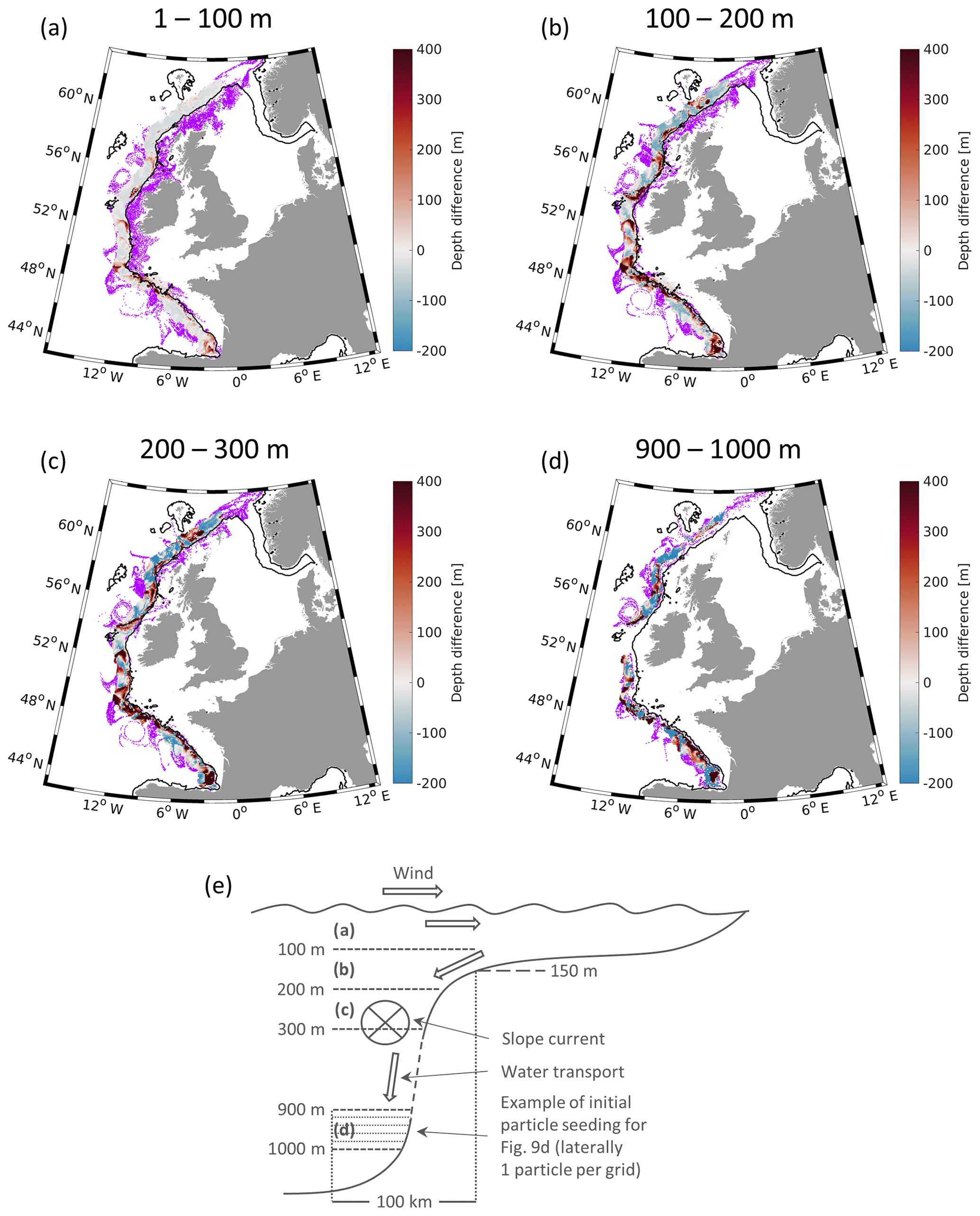
Figure 9Particle positions (purple dots) and particle depth differences with respect to the depth of release in different depth layers (colours) after 1 month (January) in 2015 computed in the control run with vertical particle seeding along the continental slope (CR-V, no. 6; see Table 1). Details of the seeding strategy can be found in Sect. 2.3. The colour coding shows the difference of the final depth minus the initial particle depth, computed as the mean difference of all particle depths seeded at the same location in the horizontal plane. All particles released in the respective depth range are taken into account. Particles were released in four depth layers: (a) 1–100 m, (b) 100–200 m, (c) 200–300 m and (d) 900–1000 m. (e) Sketched dynamics at the continental slope concluded from (a) to (d).
4.5 Dynamics at the shelf edge
The analysis below uses the results of the CR-V (experiment no. 6; see Table 1) with the seeding prescribed in a 100 km wide segment extending oceanward from the 150 m isobaths. The exchange of particles between the deep ocean and the shelf is estimated by the number of particles crossing the 200 m isobaths and the changes in their depth with respect to the depth at which they were released. The 100 km wide segment is divided vertically into four parts: from the surface to 100 m (Fig. 9a), 100–200 m (Fig. 9b), 200–300 m (Fig. 9c), and 900–1000 m (Fig. 9d). The major result of this experiment is that with increasing depth (1) the dispersion of the cloud of particles in the vicinity of the 200 m isobaths decreases, and (2) particles in the deeper layers do not penetrate onto the shelf. Many particles released above 100 m move onto the shelf; their depth remains almost unchanged or even decreases (Fig. 9a). In the three deeper intervals of release, deep oceanward transport is dominant (red stripe along the 200 m isobath in Fig. 9b, c, and d). These dynamics, which are sketched in Fig. 9e, support the results by Holt et al. (2009), Huthnance et al. (2009), and Graham et al. (2018), whose simulations also showed shelfward transport distinctive of the upper 150 m along the 200 m isobath; below 150 m, they found deep oceanward transport. The simulated exchanges between the shelf and open ocean (the extent and direction of particle propagation) are also in overall agreement with the recent results by Marsh et al. (2017), who analysed drifter observations and Lagrangian simulations at the ENWS continental slope. Down to 300 m, particles propagating away from the continental slope form filaments and eddy-like patterns as in the Bay of Biscay; another fraction of the particles are advected within the slope current. Although the latter are covered by the coloured areas, some of them are visible at the entrance of the Norwegian Trench. The underlying dynamics at the ENWS continental slope are discussed in Sect. 4.1 and 4.2.
Numerical experiments were carried out with NEMO, in which a Lagrangian module was incorporated in order to learn more about the ocean dynamics on the northwest European shelf. Lagrangian analyses in conjunction with Eulerian analyses revealed physically distinct regimes in different parts of the study area. The underlying dynamics were investigated in terms of accumulation and removal of neutrally buoyant particles solely advected by the model velocities. To quantify accumulation and removal of particles, a quantity named NCPD was introduced. The current knowledge about shelf and shelf edge processes is extended not only by analysing specific processes but also by providing a rather comprehensive description of the dynamics:
-
On the shelf the fronts act as barriers and accumulate particles. Tides affect the positions and appearance of particle accumulation in frontal areas. Vertical water transport at meridionally oriented coasts on the shelf is influenced by westerlies. Offshore-directed wind induces a NCPD smaller than 1; the situation is reversed for onshore-directed wind.
-
In the deep ocean the eddies influence the particle dynamics on short timescales (individual months); however, an annual mean of NCPD ≈1 reveals the absence of long-term stable accumulation areas. In the Bay of Biscay accumulation patterns form on longer timescales than 1 month. Tides affect the NCPD, suggesting the interaction of tides and mesoscale dynamics.
-
The shelf edge (200 m isobath) represents a transition zone from the wind- and tidally driven shallow shelf regime to a baroclinic eddy-dominated deep ocean regime. The shelf edge shows on-shelf transport in the upper layers and downwelling-like off-shelf-directed transport below 100 m. Bottom current branches tend to remove particles from the continental slope.
-
At the surface, accumulation patterns on the shelf show high variability on monthly timescales; some accumulation areas remain stable on yearly average of monthly patterns. These long-term stable zones occur mainly along the fronts of ROFIs and in the Skagerrak. At the shelf edge, particles are transported onto the shelf by westerlies. The influence of wind variability on particle accumulation is of the order of the influence of tides.
-
At the bottom, bottom currents on the shelf are mainly influenced by the topography and follow its thalweg.
The differences in the properties of the velocity field (e.g. deformation) reveal two different regimes: a shelf regime with rather little deformation and a deep ocean regime at the 10 km scale with considerable deformation. On the shelf, tidally induced deformation plays an important role in particle accumulation and dispersal. The major hypothesis, that the vertical circulation in the shallow North Sea plays a substantial role, was confirmed.
The present study demonstrates the illustrative potential of Lagrangian methods. In conjunction with traditional Eulerian analysis, Lagrangian analysis can enhance the interpretation of observed or simulated dynamics and provide a solid basis for estimating the propagation of floating marine debris.
The model codes of NEMO (https://www.nemo-ocean.eu, last access: 13 November 2018), ARIANE (http://stockage.univ-brest.fr/~grima/Ariane/, last access: 30 October 2018), and OpenDrift (https://github.com/OpenDrift/opendrift, last access: 2 April 2019) as well as the GPS drifter (Carrasco and Horstmann, 2017, https://doi.org/10.1594/PANGAEA.874511), FOAM AMM7 (https://marine.copernicus.eu, last access: 20 December 2018), HF radar (http://codm.hzg.de/codm/, last access: 5 June 2019), and OSTIA (https://resources.marine.copernicus.eu/?option=com_csw&task=results?option=com_csw&view=details&product_id=SST_GLO_SST_L4_NRT_OBSERVATIONS_010_001, last access: 20 February 2020) data are freely available. E-HYPE data can be accessed under https://hypeweb.smhi.se/ (last access: 14 October 2018) and the NWP model data under https://www.metoffice.gov.uk/ (last access: 30 September 2018). Scripts and model output can be obtained by a request to the corresponding author.
The supplement related to this article is available online at: https://doi.org/10.5194/os-16-637-2020-supplement.
MR and EVS conceived the study. MR performed the model runs and analyses and prepared the figures. MR and EVS interpreted the results, and MR prepared the article with a significant contribution from EVS.
The authors declare that they have no conflict of interest.
The authors thank the UK Met Office and Joanna Staneva for providing the NEMO AMM7 setup. We also thank Sebastian Grayek for technical support and Jens Meyerjürgens for carefully reading the article and giving important advice. We appreciate the critical and detailed reviews of Knut-Frode Dagestad and one anonymous reviewer.
This study has been supported by the project “Macroplastics Pollution in the Southern North Sea – Sources, Pathways and Abatement Strategies” (grant no. ZN3176) funded by the German Federal State of Lower Saxony.
This paper was edited by Erik van Sebille and reviewed by Knut-Frode Dagestad and one anonymous referee.
Backhaus, J.: First Results of a Three-Dimensional Model on the Dynamics in the German Bighta, in: Elsev. Oceanogr. Serie. Vol. 25, edited by: Nihoul, J. C. J., Elsevier, Amsterdam, the Netherlands, 333–349, https://doi.org/10.1016/S0422-9894(08)71138-3, 1979.
Backhaus, J. O.: A three-dimensional model for the simulation of shelf sea dynamics, Deutsche Hydrografische Zeitschrift, 38, 165–187, https://doi.org/10.1007/BF02328975, 1985.
Baschek, B., Schroeder, F., Brix, H., Riethmüller, R., Badewien, T. H., Breitbach, G., Brügge, B., Colijn, F., Doerffer, R., Eschenbach, C., Friedrich, J., Fischer, P., Garthe, S., Horstmann, J., Krasemann, H., Metfies, K., Merckelbach, L., Ohle, N., Petersen, W., Pröfrock, D., Röttgers, R., Schlüter, M., Schulz, J., Schulz-Stellenfleth, J., Stanev, E., Staneva, J., Winter, C., Wirtz, K., Wollschläger, J., Zielinski, O., and Ziemer, F.: The Coastal Observing System for Northern and Arctic Seas (COSYNA), Ocean Sci., 13, 379–410, https://doi.org/10.5194/os-13-379-2017, 2017.
Belkin, I. M., Cornillon, P. C., and Sherman, K.: Fronts in Large Marine Ecosystems, Prog. Oceanogr., 81, 223–236, https://doi.org/10.1016/j.pocean.2009.04.015, 2009.
Beron-Vera, F. J., Hadjighasem, A., Xia, Q., Olascoaga, M. J., and Haller, G.: Coherent Lagrangian swirls among submesoscale motions, P. Natl. Acad. Sci. USA, 116, 18251–18256, https://doi.org/10.1073/pnas.1701392115, 2019.
Blanke, B. and Raynaud, S.: Kinematics of the Pacific Equatorial Undercurrent: An Eulerian and Lagrangian Approach from GCM Results, J. Phys. Oceanogr., 27, 1038–1053, https://doi.org/10.1175/1520-0485(1997)027<1038:KOTPEU>2.0.CO;2, 1997.
Blanke, B., Arhan, M., Madec, G., and Roche, S.: Warm Water Paths in the Equatorial Atlantic as Diagnosed with a General Circulation Model, J. Phys. Oceanogr., 29, 2753–2768, https://doi.org/10.1175/1520-0485(1999)029<2753:WWPITE>2.0.CO;2, 1999.
Booth, D. A.: Eddies in the Rockall Trough, Oceanolog. Acta, 11, 213–219, 1988.
Bower, A. S., Lozier, M. S., Gary, S. F., and Böning, C. W.: Interior pathways of the North Atlantic meridional overturning circulation, Nature, 459, 243–247, https://doi.org/10.1038/nature07979, 2009.
Callies, U., Plüß, A., Kappenberg, J., and Kapitza, H.: Particle tracking in the vicinity of Helgoland, North Sea: a model comparison, Ocean Dynam., 61, 2121–2139, https://doi.org/10.1007/s10236-011-0474-8, 2011.
Callies, U., Groll, N., Horstmann, J., Kapitza, H., Klein, H., Maßmann, S., and Schwichtenberg, F.: Surface drifters in the German Bight: model validation considering windage and Stokes drift, Ocean Sci., 13, 799–827, https://doi.org/10.5194/os-13-799-2017, 2017.
Carrasco, R. and Horstmann, J.: German Bight surface drifter data from Heincke cruise HE 445, 2015, PANGAEA, https://doi.org/10.1594/PANGAEA.874511, 2017.
Daewel, U., Peck, M. A., Kühn, W., St. John, M. A., Alekseeva, I., and Schrum, C.: Coupling ecosystem and individual-based models to simulate the influence of environmental variability on potential growth and survival of larval sprat (Sprattus sprattus L.) in the North Sea, Fish. Oceanogr., 17, 333–351, https://doi.org/10.1111/j.1365-2419.2008.00482.x, 2008.
Dagestad, K.-F., Röhrs, J., Breivik, Ø., and Ådlandsvik, B.: OpenDrift v1.0: a generic framework for trajectory modelling, Geosci. Model Dev., 11, 1405–1420, https://doi.org/10.5194/gmd-11-1405-2018, 2018.
Davies, A. M. and Xing, J.: Modelling processes influencing shelf edge currents, mixing, across shelf exchange, and sediment movement at the shelf edge, Dynam. Atmos. Oceans, 34, 291–326, https://doi.org/10.1016/S0377-0265(01)00072-0, 2001.
Davies, A. M., Sauvel, J., and Evans, J.: Computing near coastal tidal dynamics from observations and a numerical model, Cont. Shelf Res., 4, 341–366, https://doi.org/10.1016/0278-4343(85)90047-0, 1985.
de Boer, G. J., Pietrzak, J. D., and Winterwerp, J. C.: SST observations of upwelling induced by tidal straining in the Rhine ROFI, Cont. Shelf Res., 29, 263–277, https://doi.org/10.1016/j.csr.2007.06.011, 2009.
Donlon, C. J., Martin, M., Stark, J., Roberts-Jones, J., Fiedler, E., and Wimmer, W.: The Operational Sea Surface Temperature and Sea Ice Analysis (OSTIA) system, Remote Sens. Environ., 116, 140–158, https://doi.org/10.1016/j.rse.2010.10.017, 2012.
Flament, P. and Armi, L.: The Shear, Convergence, and Thermohaline Structure of a Front, J. Phys. Oceanogr., 30, 51–66, https://doi.org/10.1175/1520-0485(2000)030<0051:TSCATS>2.0.CO;2, 2000.
Flather, R. A.: A Storm Surge Prediction Model for the Northern Bay of Bengal with Application to the Cyclone Disaster in April 1991, J. Phys. Oceanogr., 24, 172–190, https://doi.org/10.1175/1520-0485(1994)024<0172:ASSPMF>2.0.CO;2, 1994.
Froyland, G., Stuart, R. M., and van Sebille, E.: How well-connected is the surface of the global ocean?, Chaos, 24, 033126, https://doi.org/10.1063/1.4892530, 2014.
Garrett, C. J. R. and Loder, J. W.: Circulation and fronts in continental shelf seas – Dynamical aspects of shallow sea fronts, Philos. T. Roy. Soc. A, 302, 563–581, https://doi.org/10.1098/rsta.1981.0183, 1981.
Graham, J. A., Rosser, J. P., O'Dea, E., and Hewitt, H. T.: Resolving Shelf Break Exchange Around the European Northwest Shelf, Geophys. Res. Lett., 45, 12386–12395, https://doi.org/10.1029/2018GL079399, 2018.
Guihou, K., Polton, J., Harle, J., Wakelin, S., O'Dea, E., and Holt, J.: Kilometric Scale Modeling of the North West European Shelf Seas: Exploring the Spatial and Temporal Variability of Internal Tides, J. Geophys. Res.-Oceans, 123, 688–707, https://doi.org/10.1002/2017JC012960, 2018.
Gutow, L., Ricker, M., Holstein, J., Dannheim, J., Stanev, E. V., and Wolff, J.-O.: Distribution and trajectories of floating and benthic marine macrolitter in the south-eastern North Sea, Mar. Pollut. Bull., 131, 763–772, https://doi.org/10.1016/j.marpolbul.2018.05.003, 2018.
Hainbucher, D., Pohlmann, T., and Backhaus, J.: Transport of conservative passive tracers in the North Sea: first results of a circulation and transport model, Cont. Shelf Res., 7, 1161–1179, https://doi.org/10.1016/0278-4343(87)90083-5, 1987.
Haller, G. and Yuan, G.: Lagrangian coherent structures and mixing in two-dimensional turbulence, Physica D, 147, 352–370, https://doi.org/10.1016/S0167-2789(00)00142-1, 2000.
Heaps, N. S.: Density currents in a two-layered coastal system, with application to the Norwegian Coastal Current, Geophys. J. Roy. Astr. S., 63, 289–310, https://doi.org/10.1111/j.1365-246X.1980.tb02622.x, 1980.
Hill, A. E., James, I. D., Linden, P. F., Matthews, J. P., Prandle, D., Simpson, J. H., Gmitrowicz, E. M., Smeed, D. A., Lwiza, K. M. M., Durazo, R., Fox, A. D., and Bowers, D. G.: Understanding the North Sea system – Dynamics of tidal mixing fronts in the North Sea, Philos. T. Roy. Soc. A, 343, 431–446, https://doi.org/10.1098/rsta.1993.0057, 1993.
Hill, A. E., Brown, J., Fernand, L., Holt, J., Horsburgh, K. J., Proctor, R., Raine, R., and Turrell, W. R.: Thermohaline circulation of shallow tidal seas, Geophys. Res. Lett., 35, L11605, https://doi.org/10.1029/2008GL033459, 2008.
Holt, J. T. and James, I. D.: A simulation of the Southern North Sea in comparison with measurements from the North Sea Project. Part 1: Temperature, Cont. Shelf Res., 19, 1087–1112, https://doi.org/10.1016/S0278-4343(99)00015-1, 1999.
Holt, J. and Umlauf, L.: Modelling the tidal mixing fronts and seasonal stratification of the Northwest European Continental shelf, Cont. Shelf Res., 28, 887–903, https://doi.org/10.1016/j.csr.2008.01.012, 2008.
Holt, J., Wakelin, S., and Huthnance, J.: Down-welling circulation of the northwest European continental shelf: A driving mechanism for the continental shelf carbon pump, Geophys. Res. Lett., 36, L14602, https://doi.org/10.1029/2009GL038997, 2009.
Howarth, M. J.: North Sea Circulation, in: Encyclopedia of Ocean Sciences: Vol. 1, edited by: Steele, J. H., Turekian, K. K., and Thorpe, S. A, Academic Press, Oxford, UK, 1912–1921, 2001.
Huntley, H. S., Lipphardt, B. L., Jacobs, G., and Kirwan, A. D.: Clusters, deformation, and dilation: Diagnostics for material accumulation regions, J. Geophys. Res.-Oceans, 120, 6622–6636, https://doi.org/10.1002/2015JC011036, 2015.
Huthnance, J. M.: Physical oceanography of the North Sea, Ocean and Shoreline Management, 16, 199–231, https://doi.org/10.1016/0951-8312(91)90005-M, 1991.
Huthnance, J. M.: Circulation, exchange and water masses at the ocean margin: the role of physical processes at the shelf edge, Prog. Oceanogr., 35, 353–431, https://doi.org/10.1016/0079-6611(95)80003-C, 1995.
Huthnance, J. M., Holt, J. T., and Wakelin, S. L.: Deep ocean exchange with west-European shelf seas, Ocean Sci., 5, 621–634, https://doi.org/10.5194/os-5-621-2009, 2009.
Jacob, B. and Stanev, E. V.: Interactions between wind and tidally induced currents in coastal and shelf basins, Ocean Dynam., 67, 1263–1281, https://doi.org/10.1007/s10236-017-1093-9, 2017.
Koszalka, I. M. and LaCasce, J. H.: Lagrangian analysis by clustering, Ocean Dynam., 60, 957–972, https://doi.org/10.1007/s10236-010-0306-2, 2010.
Koszalka, I. M., LaCasce, J. H., Andersson, M., Orvik, K. A., and Mauritzen, C.: Surface circulation in the Nordic Seas from clustered drifters, Deep-Sea Res. Pt. I, 58, 468–485, https://doi.org/10.1016/j.dsr.2011.01.007, 2011.
Krause, G., Budeus, G., Gerdes, D., Schaumann, K., and Hesse, K.: Frontal Systems in the German Bight and their Physical and Biological Effects, in: Elsev. Oceanogr. Series, vol. 42, edited by: Nihoul, J. C. J., Elsevier, Amsterdam, the Netherlands, 119–140, https://doi.org/10.1016/S0422-9894(08)71042-0, 1986.
Le Fèvre, J.: Aspects of the Biology of Frontal Systems, Adv. Mar. Biol., 23, 163–299, 1986.
Lentz, S. J. and Fewings, M. R.: The wind- and wave-driven inner-shelf circulation, Annu. Rev. Mar. Sci., 4, 317–343, https://doi.org/10.1146/annurev-marine-120709-142745, 2012.
Lohmann, R. and Belkin, I. M.: Organic pollutants and ocean fronts across the Atlantic Ocean: A review, Prog. Oceanogr., 128, 172–184, https://doi.org/10.1016/j.pocean.2014.08.013, 2014
Madec, G.: NEMO ocean engine, Note du Pôle de modélisation, Institut Pierre-Simon Laplace (IPSL), France, 27, 2008.
Mahadevan, A.: The Impact of Submesoscale Physics on Primary Productivity of Plankton, Annu. Rev. Mar. Sci., 8, 161–184, https://doi.org/10.1146/annurev-marine-010814-015912, 2016.
Maier-Reimer, E.: Residual circulation in the North Sea due to the M2-tide and mean annual wind stress, Deutsche Hydrografische Zeitschrift, 30, 69–80, https://doi.org/10.1007/BF02227045, 1977.
Marsh, R., Haigh, I. D., Cunningham, S. A., Inall, M. E., Porter, M., and Moat, B. I.: Large-scale forcing of the European Slope Current and associated inflows to the North Sea, Ocean Sci., 13, 315–335, https://doi.org/10.5194/os-13-315-2017, 2017.
Maximenko, N., Hafner, J., Kamachi, M., and MacFadyen, A.: Numerical simulations of debris drift from the Great Japan Tsunami of 2011 and their verification with observational reports, Mar. Pollut. Bull., 132, 5–5, https://doi.org/10.1016/j.marpolbul.2018.03.056, 2018.
McWilliams, J. C.: Submesoscale currents in the ocean, P. Roy. Soc. A-Math. Phy., 472, 20160117, https://doi.org/10.1098/rspa.2016.0117, 2016.
Molinari, R. and Kirwan, A. D.: Calculations of Differential Kinematic Properties from Lagrangian Observations in the Western Caribbean Sea, J. Phys. Oceanogr., 5, 483–491, https://doi.org/10.1175/1520-0485(1975)005<0483:CODKPF>2.0.CO;2, 1975.
Neumann, D., Callies, U., and Matthies, M.: Marine litter ensemble transport simulations in the southern North Sea, Mar. Pollut. Bull., 86, 219–228, https://doi.org/10.1016/j.marpolbul.2014.07.016, 2014.
O'Dea, E. J., Arnold, A. K., Edwards, K. P., Furner, R., Hyder, P., Martin, M. J., Siddorn, J. R., Storkey, D., While, J., Holt, J. T., and Liu, H.: An operational ocean forecast system incorporating NEMO and SST data assimilation for the tidally driven European North-West shelf, J. Oper. Oceanogr., 5, 3–17, https://doi.org/10.1080/1755876X.2012.11020128, 2012.
O'Dea, E., Furner, R., Wakelin, S., Siddorn, J., While, J., Sykes, P., King, R., Holt, J., and Hewitt, H.: The CO5 configuration of the 7 km Atlantic Margin Model: large-scale biases and sensitivity to forcing, physics options and vertical resolution, Geosci. Model Dev., 10, 2947–2969, https://doi.org/10.5194/gmd-10-2947-2017, 2017.
Otto, L., Zimmerman, J. T. F., Furnes, G. K., Mork, M., Saetre, R., and Becker, G.: Review of the physical oceanography of the North Sea, Neth, J. Sea Res., 26, 161–238, https://doi.org/10.1016/0077-7579(90)90091-T, 1990.
Paparella, F., Babiano, A., Basdevant, C., Provenzale, A., and Tanga, P.: A Lagrangian study of the Antarctic polar vortex, J. Geophys. Res.-Atmos., 102, 6765–6773, https://doi.org/10.1029/96JD03377, 1997.
Pätsch, J., Burchard, H., Dieterich, C., Gräwe, U., Gröger, M., Mathis, M., Kapitza, H., Bersch, M., Moll, A., Pohlmann, T., Su, J., Ho-Hagemann, H. T. M., Schulz, A., Elizalde, A., and Eden, C.: An evaluation of the North Sea circulation in global and regional models relevant for ecosystem simulations, Ocean Model., 116, 70–95, https://doi.org/10.1016/j.ocemod.2017.06.005, 2017.
Pietrzak, J. D., de Boer, G. J., and Eleveld, M. A.: Mechanisms controlling the intra-annual mesoscale variability of SST and SPM in the southern North Sea, Cont. Shelf Res., 31, 594–610, https://doi.org/10.1016/j.csr.2010.12.014, 2011.
Pingree, R. D. and Griffiths, D. K.: Tidal fronts on the shelf seas around the British Isles, J. Geophys. Res.-Oceans, 83, 4615–4622, https://doi.org/10.1029/JC083iC09p04615, 1978.
Pohlmann, T.: A meso-scale model of the central and southern North Sea: Consequences of an improved resolution, Cont. Shelf Res., 26, 2367–2385, https://doi.org/10.1016/j.csr.2006.06.011, 2006.
Porter, M., Inall, M. E., Green, J. A. M., Simpson, J. H., Dale, A. C., and Miller, P. I.: Drifter observations in the summer time Bay of Biscay slope current, J. Marine Syst., 157, 65–74, https://doi.org/10.1016/j.jmarsys.2016.01.002, 2016.
Postma, H.: Introduction to the symposium on organic matter in the Wadden Sea, in: The role of organic matter in the Wadden Sea, edited by: Laane, R. W. P. M. and Wolff, W. J., Texel, the Netherlands, 15–22, 1984.
Reisser, J., Shaw, J., Wilcox, C., Hardesty, B. D., Proietti, M., Thums, M., and Pattiaratchi, C.: Marine Plastic Pollution in Waters around Australia: Characteristics, Concentrations, and Pathways, PLOS ONE, 8, e80466, https://doi.org/10.1371/journal.pone.0080466, 2013.
Rodhe, J.: The large-scale circulation in the Skagerrak; interpretation of some observations, Tellus A, 39A, 245–253, https://doi.org/10.3402/tellusa.v39i3.11757, 1987.
Röhrs, J., Christensen, K. H., Hole, L. R., Broström, G., Drivdal, M., and Sundby, S.: Observation-based evaluation of surface wave effects on currents and trajectory forecasts, Ocean Dynam., 62, 1519–1533, https://doi.org/10.1007/s10236-012-0576-y, 2012.
Rolinski, S.: On the dynamics of suspended matter transport in the tidal river Elbe: Description and results of a Lagrangian model, J. Geophys. Res.-Oceans, 104, 26043–26057, https://doi.org/10.1029/1999JC900230, 1999.
Schönfeld, W.: Numerical simulation of the dispersion of artificial radionuclides in the English Channel and the North Sea, J. Marine Syst., 6, 529–544, https://doi.org/10.1016/0924-7963(95)00022-H, 1995.
Simpson, J. H. and Hunter, J. R.: Fronts in the Irish Sea, Nature, 250, 404–406, https://doi.org/10.1038/250404a0, 1974.
Simpson, J. H. and Pingree, R. D.: Shallow Sea Fronts Produced by Tidal Stirring, in: Oceanic Fronts in Coastal Processes, edited by: Bowman, M. J., and Esaias, W. E., Springer, Berlin, 29–42, https://doi.org/10.1007/978-3-642-66987-3_5, 1978.
Simpson, J. H. and Sharples, J.: Introduction to the Physical and Biological Oceanography of Shelf Seas, Cambridge University Press, Cambridge, UK, 2012.
Smagorinsky, J.: General circulation experiments with the primitive equations, Mon. Weather Rev., 91, 99–164, https://doi.org/10.1175/1520-0493(1963)091<0099:GCEWTP>2.3.CO;2, 1963.
Stanev, E. V. and Ricker, M.: Interactions between barotropic tides and mesoscale processes in deep ocean and shelf regions, Ocean Dynam., 70, 713–728, https://doi.org/10.1007/s10236-020-01348-6, 2020.
Stanev, E. V., Ziemer, F., Schulz-Stellenfleth, J., Seemann, J., Staneva, J., and Gurgel, K. W.: Blending Surface Currents from HF Radar Observations and Numerical Modelling: Tidal Hindcasts and Forecasts, J. Atmos. Ocean. Tech., 32, 256–281, https://doi.org/10.1175/JTECH-D-13-00164.1, 2015.
Stanev, E. V., Badewien, T. H., Freund, H., Grayek, S., Hahner, F., Meyerjürgens, J., Ricker, M., Schöneich-Argent, R. I., Wolff, J.-O., and Zielinski, O.: Extreme westward surface drift in the North Sea: Public reports of stranded drifters and Lagrangian tracking, Cont. Shelf Res., 177, 24–32, https://doi.org/10.1016/j.csr.2019.03.003, 2019.
van Aken, H. M.: The hydrography of the mid-latitude Northeast Atlantic Ocean – Part III: the subducted thermocline water mass, Deep-Sea Res. Pt. I, 48, 237–267, https://doi.org/10.1016/S0967-0637(00)00059-5, 2001.
van Aken, H. M., van Heijst, G. J. F., and Maas, L. R. M.: Observations of fronts in the North Sea, J. Mar. Res., 45, 579–600, https://doi.org/10.1357/002224087788326830, 1987.
van der Molen, J., García-García, L. M., Whomersley, P., Callaway, A., Posen, P. E., and Hyder, K.: Connectivity of larval stages of sedentary marine communities between hard substrates and offshore structures in the North Sea, Sci. Rep.-UK, 8, 14772, https://doi.org/10.1038/s41598-018-32912-2, 2018.
van Sebille, E., England, M. H., and Froyland, G.: Origin, dynamics and evolution of ocean garbage patches from observed surface drifters, Environ. Res. Lett., 7, 044040, https://doi.org/10.1088/1748-9326/7/4/044040, 2012.
van Sebille, E., Wilcox, C., Lebreton, L., Maximenko, N., Hardesty, B. D., van Franeker, J. A., Eriksen, M., Siegel, D., Galgani, F., and Law, K. L.: A global inventory of small floating plastic debris, Environ. Res. Lett., 10, 124006, https://doi.org/10.1088/1748-9326/10/12/124006, 2015.
van Sebille, E., Griffies, S. M., Abernathey, R., Adams, T. P., Berloff, P., Biastoch, A., Blanke, B., Chassignet, E. P., Cheng, Y., Cotter, C. J., Deleersnijder, E., Döös, K., Drake, H. F., Drijfhout, S., Gary, S. F., Heemink, A. W., Kjellsson, J., Koszalka, I. M., Lange, M., Lique, C., MacGilchrist, G. A., Marsh, R., Adame, C. G. M., McAdam, R., Nencioli, F., Paris, C. B., Piggott, M. D., Polton, J. A., Rühs, S., Shah, S. H. A. M., Thomas, M. D., Wang, J., Wolfram, P. J., Zanna, L., and Zika, J. D.: Lagrangian ocean analysis: Fundamentals and practices, Ocean Model., 121, 49–75, https://doi.org/10.1016/j.ocemod.2017.11.008, 2018.
Zhang, Y. J., Stanev, E. V., and Grashorn, S.: Unstructured-grid model for the North Sea and Baltic Sea: Validation against observations, Ocean Model., 97, 91–108, https://doi.org/10.1016/j.ocemod.2015.11.009, 2016.
normalised cumulative particle densitymeasures particle accumulation. Yearly averages reveal no surface accumulation areas in the deep ocean and elongated patterns on the shelf mainly along fronts. Sensitivity experiments show the influence of tides and wind, unveiling important vertical dynamics in coastal areas.